Chapter 27: Integer Factoring Algorithms

Chapter 27: Integer Factoring Algorithms#

The security of RSA rests on the presumed hardness of factoring large integers. In this chapter we survey the main algorithms that have been developed to attack this problem, implement several of them from scratch, and experimentally compare their performance. We trace the historical arc from the ancient method of trial division through modern sub-exponential sieves, illustrating how each advance exploits a different structural weakness of the target composite.

27.1 Historical Overview#

Integer factorisation has been studied for centuries. The key milestones are:

Year	Algorithm	Complexity	Notes
Antiquity	Trial division	\(O(\sqrt{n})\)	Exhaustive search up to \(\sqrt{n}\)
1643	Fermat’s method	\(O(\sqrt{n})\) worst case	Exploits factorisations \(n = a^2 - b^2\)
1974	Pollard \(p-1\)	\(O(B \log B \log^2 n)\)	Exploits smooth \(p-1\)
1975	Pollard’s rho	\(O(n^{1/4})\) heuristic	Birthday-paradox collision
1981	Quadratic Sieve (QS)	\(L_n[1/2, 1]\)	First sub-exponential general method
1993	General Number Field Sieve (GNFS)	\(L_n[1/3, (64/9)^{1/3}]\)	Fastest known general algorithm

Here \(L_n[\alpha, c] = \exp\bigl(c\,(\ln n)^{\alpha}\,(\ln\ln n)^{1-\alpha}\bigr)\) is the standard L-notation for sub-exponential complexity.

Key Insight

No general-purpose factoring algorithm is known to run in polynomial time on a classical computer. Shor’s quantum algorithm achieves polynomial time, which is why quantum computing poses a threat to RSA.

27.2 The Complexity Landscape#

Let us visualise how the different complexity classes scale with the number of digits \(d = \lfloor \log_{10} n \rfloor + 1\) of the integer \(n\).

../_images/cacf138770e471fa8c5e27ad5b80ba3d5564ae3aa589e49f194c3bc54f674a1d.png

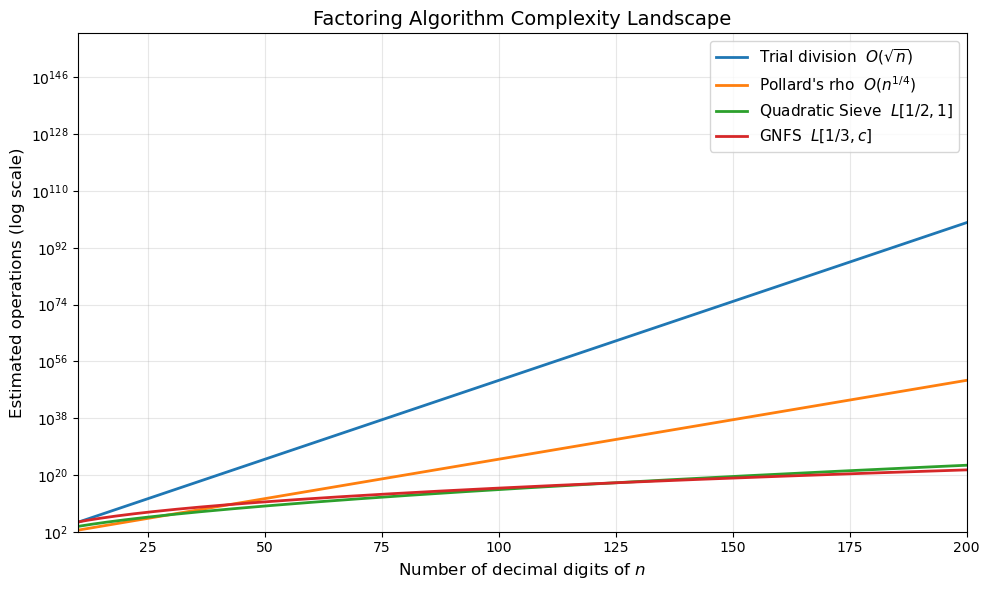
The chart shows a dramatic separation: trial division and Pollard’s rho are exponential in the digit count, while the Quadratic Sieve and GNFS are sub-exponential. For numbers beyond about 100 digits, only the sieve methods are feasible.

27.3 Trial Division#

The simplest factoring method: test every integer \(d = 2, 3, 5, 7, 11, \ldots\) up to \(\lfloor\sqrt{n}\rfloor\). If \(d \mid n\), then \(d\) is a factor.

Complexity: \(O(\sqrt{n})\) trial divisions in the worst case (when \(n\) is prime or a product of two primes of similar size).

When trial division is enough

Trial division is perfectly adequate for removing small prime factors. Many practical factoring pipelines begin with trial division up to some bound \(B\), then switch to a more sophisticated method for the remaining cofactor.

import math

def trial_division(n):
    """
    Return a non-trivial factor of n by trial division, or n itself if n is prime.
    Tests 2, then odd numbers 3, 5, 7, ... up to floor(sqrt(n)).
    """
    if n < 2:
        return n
    if n % 2 == 0:
        return 2
    d = 3
    while d * d <= n:
        if n % d == 0:
            return d
        d += 2
    return n  # n is prime

# Quick tests
test_cases = [15, 221, 1009 * 1013, 2 ** 31 - 1]
for tc in test_cases:
    f = trial_division(tc)
    if f == tc:
        print(f"trial_division({tc}) -> {tc} is prime")
    else:
        print(f"trial_division({tc}) -> {f} x {tc // f}")

trial_division(15) -> 3 x 5
trial_division(221) -> 13 x 17
trial_division(1022117) -> 1009 x 1013
trial_division(2147483647) -> 2147483647 is prime

27.4 Pollard’s Rho Algorithm#

Pollard’s rho (1975) uses the birthday paradox to find a collision modulo an unknown factor \(p\) of \(n\). The idea:

Define a pseudo-random sequence \(x_{i+1} = f(x_i) \pmod{n}\) where typically \(f(x) = x^2 + c\).
Because the sequence is eventually periodic modulo \(p\), by the birthday bound we expect a collision \(x_i \equiv x_j \pmod{p}\) after roughly \(O(\sqrt{p})\) steps.
Detect the collision using Floyd’s cycle detection (tortoise and hare) by checking \(\gcd(|x_i - x_{2i}|,\, n) > 1\).

Expected complexity: \(O(n^{1/4} \operatorname{polylog} n)\) for finding the smallest prime factor of \(n\).

Why “rho”?

The sequence, when drawn as a graph, forms a shape like the Greek letter \(\rho\): a tail leading into a cycle.

import math

def pollard_rho(n, c=1, max_iter=10**6):
    """
    Pollard's rho with Floyd's cycle detection.
    Uses f(x) = x^2 + c  (mod n).
    Returns a non-trivial factor or None.
    """
    if n % 2 == 0:
        return 2
    f = lambda x: (x * x + c) % n
    x = 2  # tortoise
    y = 2  # hare
    d = 1
    while d == 1:
        x = f(x)
        y = f(f(y))
        d = math.gcd(abs(x - y), n)
        max_iter -= 1
        if max_iter == 0:
            return None
    return d if d != n else None

# Test on moderately large composites
composites = [
    ("8051", 8051),
    ("1000003 * 1000033", 1000003 * 1000033),
    ("104729 * 104743", 104729 * 104743),
]
for label, n in composites:
    factor = pollard_rho(n)
    if factor:
        print(f"pollard_rho({label}) = {factor} x {n // factor}")
    else:
        print(f"pollard_rho({label}) failed (try different c)")

pollard_rho(8051) = 97 x 83
pollard_rho(1000003 * 1000033) = 1000033 x 1000003
pollard_rho(104729 * 104743) = 104729 x 104743

27.4.1 Visualising the Rho Trajectory#

We trace the sequence \(x_0, x_1, x_2, \ldots\) modulo a small composite to see the characteristic tail-and-cycle (rho) shape.

Show code cell source Hide code cell source

import numpy as np
import matplotlib.pyplot as plt
import math

def rho_trajectory(n, c=1, x0=2, max_steps=200):
    """Record the rho sequence and detect the cycle."""
    f = lambda x: (x * x + c) % n
    seq = [x0]
    x = x0
    for _ in range(max_steps):
        x = f(x)
        seq.append(x)
        # simple cycle check
        if x in seq[:-1]:
            break
    return seq

n_small = 551  # 19 * 29
seq = rho_trajectory(n_small, c=1, x0=2)

# Find cycle start
seen = {}
tail_len = 0
for i, v in enumerate(seq):
    if v in seen:
        tail_len = seen[v]
        cycle_len = i - tail_len
        break
    seen[v] = i

# Layout: place tail nodes in a line, cycle nodes on a circle
tail_nodes = seq[:tail_len]
cycle_nodes = seq[tail_len:tail_len + cycle_len]

fig, ax = plt.subplots(figsize=(10, 7))

# Cycle positions on a circle
cx, cy = 4.0, 0.0
radius = 2.0
angles = np.linspace(np.pi / 2, np.pi / 2 - 2 * np.pi, cycle_len, endpoint=False)
cycle_x = cx + radius * np.cos(angles)
cycle_y = cy + radius * np.sin(angles)

# Tail positions in a line leading to the cycle start
if tail_len > 0:
    tail_x = np.linspace(cx - radius - tail_len * 0.8, cx + radius * np.cos(angles[0]), tail_len, endpoint=False)
    tail_y = np.full(tail_len, cy + radius * np.sin(angles[0]))
else:
    tail_x, tail_y = np.array([]), np.array([])

all_x = np.concatenate([tail_x, cycle_x])
all_y = np.concatenate([tail_y, cycle_y])

# Draw arrows
total = len(all_x)
for i in range(total - 1):
    dx = all_x[i + 1] - all_x[i]
    dy = all_y[i + 1] - all_y[i]
    color = 'steelblue' if i < tail_len else 'crimson'
    ax.annotate('', xy=(all_x[i + 1], all_y[i + 1]),
                xytext=(all_x[i], all_y[i]),
                arrowprops=dict(arrowstyle='->', color=color, lw=1.5))

# Close the cycle
if cycle_len > 1:
    ax.annotate('', xy=(cycle_x[0], cycle_y[0]),
                xytext=(cycle_x[-1], cycle_y[-1]),
                arrowprops=dict(arrowstyle='->', color='crimson', lw=1.5))

# Draw nodes
for i in range(total):
    color = 'lightblue' if i < tail_len else 'lightsalmon'
    ax.plot(all_x[i], all_y[i], 'o', markersize=20, color=color,
            markeredgecolor='black', markeredgewidth=1.0, zorder=5)
    label = seq[i] if i < len(seq) else ''
    ax.text(all_x[i], all_y[i], str(label), ha='center', va='center',
            fontsize=7, fontweight='bold', zorder=6)

ax.set_title(f"Pollard's Rho Trajectory for $n = {n_small}$\n"
             f"Tail length = {tail_len},  Cycle length = {cycle_len}",
             fontsize=13)
ax.set_aspect('equal')
ax.axis('off')
plt.tight_layout()
plt.savefig('fig_ch27_rho_trajectory.png', dpi=150)
plt.show()

print(f"Sequence (first {min(30, len(seq))} values): {seq[:30]}")
print(f"Tail length: {tail_len}, Cycle length: {cycle_len}")

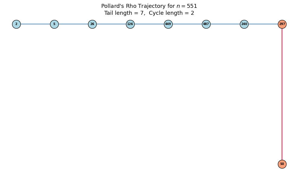
../_images/24898dee26845b2d176aa47e41e6820e5607085b88348089ca84b2210e8218a1.png

Sequence (first 10 values): [2, 5, 26, 126, 449, 487, 240, 297, 50, 297]
Tail length: 7, Cycle length: 2

27.5 Pollard’s \(p-1\) Method#

If \(p\) is a prime factor of \(n\) and \(p - 1\) is \(B\)-smooth (all prime factors \(\le B\)), then for \(M = \text{lcm}(1, 2, \ldots, B) = \prod_{\text{primes } q \le B} q^{\lfloor \log_q B \rfloor}\), Fermat’s little theorem gives

\[ a^M \equiv 1 \pmod{p}\]

so \(\gcd(a^M - 1,\, n)\) will reveal \(p\) (or a multiple of \(p\)).

Vulnerability of smooth primes

RSA key generation typically selects primes \(p\) and \(q\) such that \(p-1\) and \(q-1\) have large prime factors, making Pollard’s \(p-1\) method ineffective. Using safe primes \(p = 2q + 1\) for prime \(q\) is one common approach, but it is not the only secure strategy. Other approaches ensure that \(p - 1\) has at least one large prime factor. If \(p - 1\) is smooth (all small factors), the \(p - 1\) method will factor \(n\) quickly.

import math

def sieve_primes(limit):
    """Simple sieve of Eratosthenes up to limit."""
    is_prime = [True] * (limit + 1)
    is_prime[0] = is_prime[1] = False
    for i in range(2, int(limit**0.5) + 1):
        if is_prime[i]:
            for j in range(i*i, limit + 1, i):
                is_prime[j] = False
    return [i for i in range(2, limit + 1) if is_prime[i]]

def pollard_p_minus_1(n, B):
    """
    Pollard's p-1 method with smoothness bound B.
    Returns a non-trivial factor or None.
    """
    a = 2
    primes = sieve_primes(B)
    for p in primes:
        # Raise to p^k where p^k <= B
        pk = p
        while pk <= B:
            a = pow(a, p, n)
            pk *= p
    d = math.gcd(a - 1, n)
    if 1 < d < n:
        return d
    return None

# Test: n = p * q where p-1 is smooth
# p = 1009 (p-1 = 1008 = 2^4 * 3^2 * 7, B-smooth for B >= 7)
# q = 100003 (q-1 = 100002 = 2 * 3 * 16667, has large factor)
n_test = 1009 * 100003
print(f"n = {n_test} = 1009 x 100003")
print(f"1009 - 1 = 1008 = 2^4 * 3^2 * 7  (7-smooth)")
print(f"100003 - 1 = 100002 = 2 * 3 * 16667  (not smooth)")
print()

for B in [5, 7, 10, 50, 100]:
    f = pollard_p_minus_1(n_test, B)
    print(f"B = {int(B):>4d}:  factor = {f}")

n = 100903027 = 1009 x 100003
1009 - 1 = 1008 = 2^4 * 3^2 * 7  (7-smooth)
100003 - 1 = 100002 = 2 * 3 * 16667  (not smooth)

B =    5:  factor = None
B =    7:  factor = None
B =   10:  factor = 1009
B =   50:  factor = 1009
B =  100:  factor = 1009

27.6 Fermat’s Factoring Method#

Fermat observed that every odd composite \(n\) can be written as \(n = a^2 - b^2 = (a-b)(a+b)\). Starting from \(a = \lceil\sqrt{n}\rceil\), we increment \(a\) and check whether \(a^2 - n\) is a perfect square.

Key property: Fermat’s method is fast when the two factors are close to \(\sqrt{n}\), but degenerates to trial division or worse when they are far apart.

RSA implication

If the two RSA primes \(p\) and \(q\) are chosen too close together (i.e. \(|p - q| < n^{1/4}\)), Fermat’s method factors \(n\) almost instantly. This is why RSA standards require \(|p - q| > 2^{(k/2) - 100}\) for a \(k\)-bit modulus.

import math

def is_perfect_square(n):
    """Check if n is a perfect square using integer square root."""
    if n < 0:
        return False, 0
    r = math.isqrt(n)
    if r * r == n:
        return True, r
    return False, 0

def fermat_factor(n, max_iter=10**6):
    """
    Fermat's factoring method.
    Returns (p, q) with p <= q, or (n, 1) if no factor is found.
    """
    if n % 2 == 0:
        return (2, n // 2)
    a = math.isqrt(n)
    if a * a == n:
        return (a, a)
    a += 1  # ceil(sqrt(n))
    for _ in range(max_iter):
        b2 = a * a - n
        is_sq, b = is_perfect_square(b2)
        if is_sq:
            p, q = a - b, a + b
            if p > 1 and q > 1:
                return (min(p, q), max(p, q))
        a += 1
    return (n, 1)

# Test with close primes vs far-apart primes
close_p, close_q = 10007, 10009  # twin-ish primes
far_p, far_q = 3, 33372239       # very unbalanced

n_close = close_p * close_q
n_far = far_p * far_q

import time

for label, n_val in [(f"{close_p} x {close_q}", n_close),
                      (f"{far_p} x {far_q}", n_far)]:
    t0 = time.perf_counter()
    p, q = fermat_factor(n_val)
    dt = time.perf_counter() - t0
    print(f"fermat_factor({label}) = ({p}, {q})  [{float(dt*1e6):.1f} us]")

fermat_factor(10007 x 10009) = (10007, 10009)  [4.5 us]

fermat_factor(3 x 33372239) = (100116717, 1)  [157814.2 us]

27.7 Quadratic Sieve – Conceptual Overview#

The Quadratic Sieve (Pomerance, 1981) was the fastest general-purpose factoring algorithm before GNFS and remains simpler to implement.

Core idea#

Find integers \(x_1, x_2, \ldots\) such that

\[ x_i^2 \equiv y_i \pmod{n}\]

where each \(y_i\) is smooth (factors over a small factor base). Then use linear algebra over \(\mathbb{F}_2\) to find a subset whose product is a perfect square:

\[ \prod y_i = b^2, \qquad \prod x_i = a\]

giving \(a^2 \equiv b^2 \pmod{n}\), and hopefully \(\gcd(a - b, n)\) is a non-trivial factor.

Complexity#

\[ L_n\left[\frac{1}{2},\, 1\right] = \exp\bigl((\ln n)^{1/2}(\ln\ln n)^{1/2}\bigr)\]

Sieving step

The “sieve” in Quadratic Sieve refers to a sieving procedure (analogous to the Sieve of Eratosthenes) used to quickly identify smooth values among the \(y_i\), avoiding expensive trial factorisation of each candidate.

27.8 General Number Field Sieve (GNFS) – Conceptual Overview#

The GNFS is the asymptotically fastest known algorithm for factoring general integers. It was used to factor RSA-250 (250 decimal digits, 829 bits) in 2020.

High-level steps#

Polynomial selection: Choose two irreducible polynomials \(f(x)\) and \(g(x)\) sharing a common root \(m\) modulo \(n\).
Sieving: Search for pairs \((a, b)\) such that both \(F(a, b)\) and \(G(a, b)\) (the homogenised polynomials) are smooth.
Linear algebra: Build an exponent matrix over \(\mathbb{F}_2\) and find dependencies using the Block Lanczos or Block Wiedemann algorithm.
Square root: Compute algebraic and rational square roots to obtain the final congruence \(a^2 \equiv b^2 \pmod{n}\).

Complexity#

\[L_n\left[\frac{1}{3},\, \left(\frac{64}{9}\right)^{1/3}\right] \approx L_n[0.333,\; 1.923]\]

Scale of GNFS computations

The RSA-250 factorisation required approximately 2700 CPU core-years of computation. The sieving step was distributed across thousands of machines worldwide. The linear algebra step alone (on a matrix of dimension \(\sim 2 \times 10^8\)) took several months on a dedicated cluster.

27.9 Timing Comparison: Trial Division vs Pollard’s Rho vs \(p-1\)#

We compare the three implemented algorithms on composites of increasing size. For each \(n = p \times q\), we measure wall-clock time.

Show code cell source Hide code cell source

import numpy as np
import matplotlib.pyplot as plt
import math
import time

# --- Re-define algorithms in this cell for self-containment ---
def trial_division(n):
    if n < 2:
        return n
    if n % 2 == 0:
        return 2
    d = 3
    while d * d <= n:
        if n % d == 0:
            return d
        d += 2
    return n

def pollard_rho(n, c=1, max_iter=10**7):
    if n % 2 == 0:
        return 2
    f = lambda x: (x * x + c) % n
    x = y = 2
    d = 1
    while d == 1:
        x = f(x)
        y = f(f(y))
        d = math.gcd(abs(x - y), n)
        max_iter -= 1
        if max_iter == 0:
            return None
    return d if d != n else None

def sieve_primes(limit):
    is_prime = [True] * (limit + 1)
    is_prime[0] = is_prime[1] = False
    for i in range(2, int(limit**0.5) + 1):
        if is_prime[i]:
            for j in range(i*i, limit + 1, i):
                is_prime[j] = False
    return [i for i in range(2, limit + 1) if is_prime[i]]

def pollard_p_minus_1(n, B):
    a = 2
    primes = sieve_primes(B)
    for p in primes:
        pk = p
        while pk <= B:
            a = pow(a, p, n)
            pk *= p
    d = math.gcd(a - 1, n)
    if 1 < d < n:
        return d
    return None

# Test composites: products of two primes of similar magnitude
prime_pairs = [
    (101, 103),
    (1009, 1013),
    (10007, 10009),
    (100003, 100019),
    (1000003, 1000033),
    (10000019, 10000079),
]

digits_list = []
times_td = []
times_rho = []
times_pm1 = []

B_bound = 500  # smoothness bound for p-1

for p, q in prime_pairs:
    n = p * q
    d = len(str(n))
    digits_list.append(d)

    # Trial division
    t0 = time.perf_counter()
    for _ in range(10):
        trial_division(n)
    times_td.append((time.perf_counter() - t0) / 10)

    # Pollard rho
    t0 = time.perf_counter()
    for _ in range(10):
        pollard_rho(n)
    times_rho.append((time.perf_counter() - t0) / 10)

    # Pollard p-1 (may not always succeed)
    t0 = time.perf_counter()
    for _ in range(10):
        pollard_p_minus_1(n, B_bound)
    times_pm1.append((time.perf_counter() - t0) / 10)

# Convert to microseconds
times_td_us = [t * 1e6 for t in times_td]
times_rho_us = [t * 1e6 for t in times_rho]
times_pm1_us = [t * 1e6 for t in times_pm1]

fig, ax = plt.subplots(figsize=(10, 6))
x_pos = np.arange(len(digits_list))
width = 0.25

ax.bar(x_pos - width, times_td_us, width, label='Trial Division', color='steelblue')
ax.bar(x_pos, times_rho_us, width, label="Pollard's Rho", color='coral')
ax.bar(x_pos + width, times_pm1_us, width, label="Pollard's $p-1$ (B=500)", color='seagreen')

ax.set_xlabel('Digits of $n$', fontsize=12)
ax.set_ylabel('Time ($\\mu$s)', fontsize=12)
ax.set_title('Factoring Time Comparison', fontsize=14)
ax.set_xticks(x_pos)
ax.set_xticklabels(digits_list)
ax.set_yscale('log')
ax.legend(fontsize=11)
ax.grid(True, axis='y', alpha=0.3)
plt.tight_layout()
plt.savefig('fig_ch27_timing_comparison.png', dpi=150)
plt.show()

print(f"{'Digits':>6s} {'Trial (us)':>12s} {'Rho (us)':>12s} {'p-1 (us)':>12s}")
for i in range(len(digits_list)):
    print(f"{int(digits_list[i]):>6d} {float(times_td_us[i]):>12.1f} {float(times_rho_us[i]):>12.1f} {float(times_pm1_us[i]):>12.1f}")

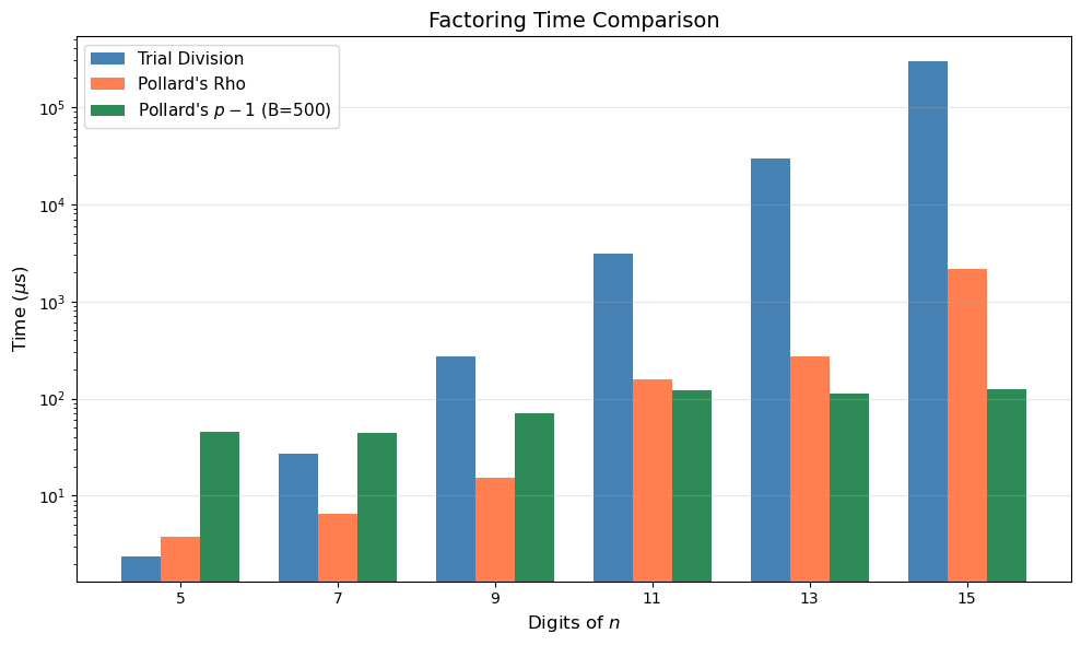
../_images/f2e5db68a2bcfabe7923c3b436c620b8b66f685120918c082a813f0c45764819.png

Digits   Trial (us)     Rho (us)     p-1 (us)
        2.4          3.7         45.2
       27.1          6.6         44.6
      275.1         15.3         70.2
     3070.5        159.7        121.1
    29729.4        270.9        113.0
   296181.6       2154.7        124.4

Observation

Pollard’s rho scales much better than trial division as \(n\) grows, confirming its \(O(n^{1/4})\) vs \(O(n^{1/2})\) advantage. The \(p-1\) method has roughly constant time (determined by \(B\)) but only succeeds when \(p - 1\) happens to be \(B\)-smooth.

27.10 Experiment: \(p-1\) Success Rate vs Smoothness Bound#

We generate many random composites \(n = p \times q\) (with \(p, q\) random primes around \(10^6\)) and measure how often the \(p - 1\) method succeeds for various values of the smoothness bound \(B\).

Show code cell source Hide code cell source

import numpy as np
import matplotlib.pyplot as plt
import math

def sieve_primes(limit):
    is_prime_arr = [True] * (limit + 1)
    is_prime_arr[0] = is_prime_arr[1] = False
    for i in range(2, int(limit**0.5) + 1):
        if is_prime_arr[i]:
            for j in range(i*i, limit + 1, i):
                is_prime_arr[j] = False
    return [i for i in range(2, limit + 1) if is_prime_arr[i]]

def pollard_p_minus_1(n, B):
    a = 2
    primes = sieve_primes(B)
    for p in primes:
        pk = p
        while pk <= B:
            a = pow(a, p, n)
            pk *= p
    d = math.gcd(a - 1, n)
    if 1 < d < n:
        return d
    return None

# Collect primes in range [10^5, 10^6] to build random composites
all_primes = sieve_primes(1000000)
candidate_primes = [p for p in all_primes if p >= 100000]

rng = np.random.default_rng(42)
num_trials = 200
B_values = [10, 20, 50, 100, 200, 500, 1000, 2000, 5000, 10000]

# Pre-generate composites
indices = rng.integers(0, len(candidate_primes), size=(num_trials, 2))
composites = [(candidate_primes[i], candidate_primes[j])
              for i, j in indices if candidate_primes[i] != candidate_primes[j]]
composites = composites[:num_trials]

success_rates = []
for B in B_values:
    successes = 0
    for p, q in composites:
        n = p * q
        if pollard_p_minus_1(n, B) is not None:
            successes += 1
    success_rates.append(successes / len(composites) * 100)

fig, ax = plt.subplots(figsize=(9, 5))
ax.plot(B_values, success_rates, 'o-', color='teal', linewidth=2, markersize=8)
ax.set_xscale('log')
ax.set_xlabel('Smoothness bound $B$', fontsize=12)
ax.set_ylabel('Success rate (%)', fontsize=12)
ax.set_title("Pollard's $p-1$: Success Rate vs Smoothness Bound\n"
             f"({num_trials} composites, primes in $[10^5, 10^6]$)", fontsize=13)
ax.set_ylim(-2, 105)
ax.grid(True, alpha=0.3)
plt.tight_layout()
plt.savefig('fig_ch27_pm1_success.png', dpi=150)
plt.show()

for B, sr in zip(B_values, success_rates):
    print(f"B = {int(B):>6d}:  success rate = {float(sr):5.1f}%")

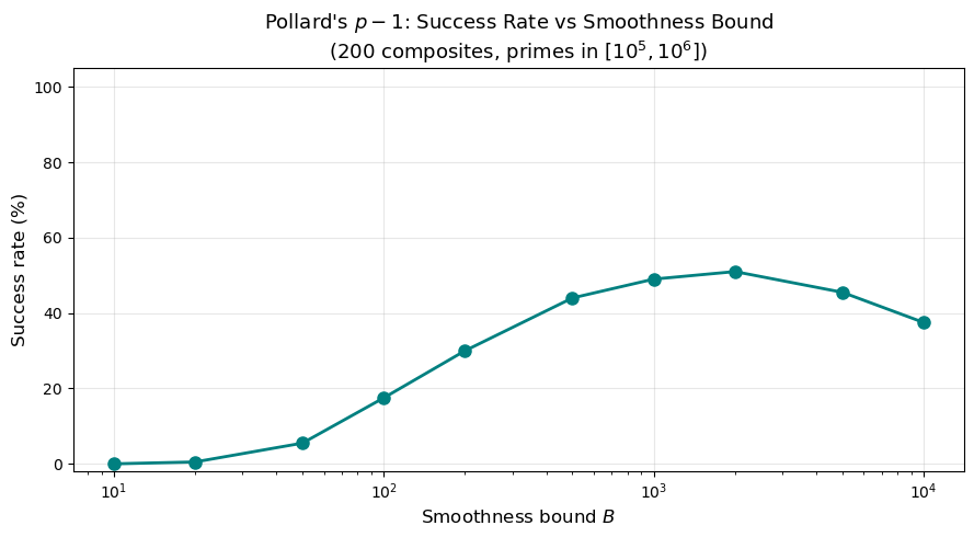
../_images/638d60abb0ac5b0c432a9a695effaa2a849864d9ee049a50a859afd433531f9a.png

B =     10:  success rate =   0.0%
B =     20:  success rate =   0.5%
B =     50:  success rate =   5.5%
B =    100:  success rate =  17.5%
B =    200:  success rate =  30.0%
B =    500:  success rate =  44.0%
B =   1000:  success rate =  49.0%
B =   2000:  success rate =  51.0%
B =   5000:  success rate =  45.5%
B =  10000:  success rate =  37.5%

As \(B\) increases, more primes \(p\) have \(B\)-smooth \(p - 1\), so the success rate rises. But increasing \(B\) also increases the running time linearly, creating a trade-off.

27.11 Historical Factoring Records#

The following chart shows the progression of factoring records over time, illustrating both algorithmic and hardware advances.

../_images/d1c7047ec7b3588adfdaec01fa69a2642b300503817c44c48d3fb498af2657fe.png

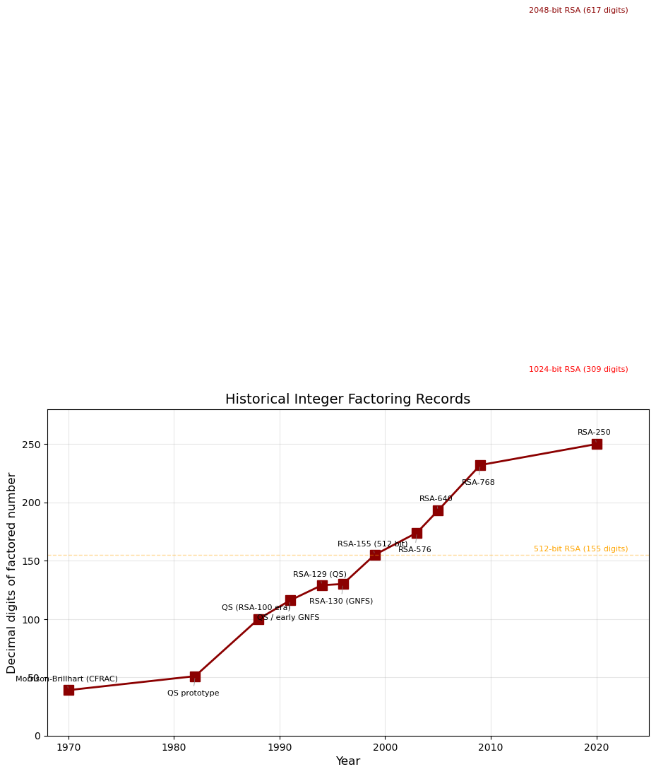
The current record (RSA-250, 829 bits) is still far from the 2048-bit keys used in practice. Extrapolating the trend, 2048-bit RSA is expected to remain safe against classical attacks for the foreseeable future.

27.12 Experiment: Factoring Difficulty vs Number of Digits#

We measure average factoring time (using Pollard’s rho) as a function of the number of digits of \(n\), verifying the expected \(O(n^{1/4})\) scaling.

Show code cell source Hide code cell source

import numpy as np
import matplotlib.pyplot as plt
import math
import time

def pollard_rho_timed(n, c=1, max_iter=10**7):
    if n % 2 == 0:
        return 2
    f = lambda x: (x * x + c) % n
    x = y = 2
    d = 1
    while d == 1:
        x = f(x)
        y = f(f(y))
        d = math.gcd(abs(x - y), n)
        max_iter -= 1
        if max_iter == 0:
            return None
    return d if d != n else None

def sieve_primes_local(limit):
    is_p = [True] * (limit + 1)
    is_p[0] = is_p[1] = False
    for i in range(2, int(limit**0.5) + 1):
        if is_p[i]:
            for j in range(i*i, limit + 1, i):
                is_p[j] = False
    return [i for i in range(2, limit + 1) if is_p[i]]

# Build prime list
all_p = sieve_primes_local(10**7)

# Group primes by digit count to form composites of desired size
digit_targets = [4, 6, 8, 10, 12, 14]
results_digits = []
results_times = []

rng = np.random.default_rng(123)
num_samples = 30

for target_d in digit_targets:
    # Each factor has ~target_d/2 digits
    half_d = target_d // 2
    lo = 10 ** (half_d - 1)
    hi = 10 ** half_d
    cand = [p for p in all_p if lo <= p < hi]
    if len(cand) < 2:
        continue

    elapsed = []
    for _ in range(num_samples):
        idx = rng.integers(0, len(cand), size=2)
        p, q = cand[idx[0]], cand[idx[1]]
        if p == q:
            continue
        n = p * q
        t0 = time.perf_counter()
        pollard_rho_timed(n)
        elapsed.append(time.perf_counter() - t0)

    results_digits.append(target_d)
    results_times.append(np.mean(elapsed) * 1e6)  # microseconds

fig, axes = plt.subplots(1, 2, figsize=(13, 5))

# Linear scale
axes[0].bar(range(len(results_digits)), results_times, color='coral',
            tick_label=results_digits, edgecolor='black', linewidth=0.5)
axes[0].set_xlabel('Digits of $n$', fontsize=12)
axes[0].set_ylabel('Mean time ($\\mu$s)', fontsize=12)
axes[0].set_title("Pollard's Rho: Time vs Digits (linear)", fontsize=13)
axes[0].grid(True, axis='y', alpha=0.3)

# Log scale with theoretical n^{1/4} reference
axes[1].semilogy(results_digits, results_times, 'o-', color='coral',
                 linewidth=2, markersize=8, label='Measured')
# Reference: n^{1/4} ~ 10^{d/4}
ref = [10 ** (d / 4) * results_times[0] / (10 ** (results_digits[0] / 4))
       for d in results_digits]
axes[1].semilogy(results_digits, ref, '--', color='gray', linewidth=1.5,
                 label='$\\propto n^{1/4}$ reference')
axes[1].set_xlabel('Digits of $n$', fontsize=12)
axes[1].set_ylabel('Mean time ($\\mu$s, log scale)', fontsize=12)
axes[1].set_title("Pollard's Rho: Scaling Verification", fontsize=13)
axes[1].legend(fontsize=11)
axes[1].grid(True, alpha=0.3)

plt.tight_layout()
plt.savefig('fig_ch27_rho_scaling.png', dpi=150)
plt.show()

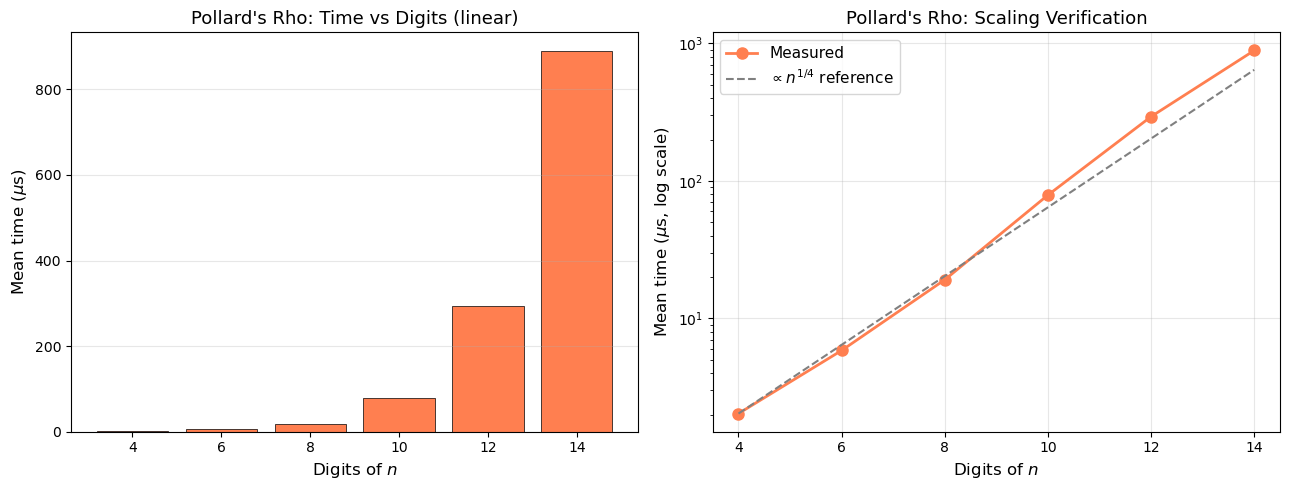
../_images/d37a22496573fef9a1a9382b923962fda288624e0276835156fc67704393cfbe.png

The measured times closely follow the \(n^{1/4}\) reference curve, confirming the heuristic complexity of Pollard’s rho algorithm.

27.13 Pollard’s Rho: Step Count Histogram#

We collect the number of iterations needed by Pollard’s rho on many random composites and compare the distribution to the birthday-bound prediction \(\approx \sqrt{\pi p / 2}\).

Show code cell source Hide code cell source

import numpy as np
import matplotlib.pyplot as plt
import math

def pollard_rho_count(n, c=1, max_iter=10**7):
    """Pollard rho returning (factor, iteration_count)."""
    if n % 2 == 0:
        return 2, 1
    f = lambda x: (x * x + c) % n
    x = y = 2
    d = 1
    count = 0
    while d == 1:
        x = f(x)
        y = f(f(y))
        d = math.gcd(abs(x - y), n)
        count += 1
        if count >= max_iter:
            return None, count
    return (d if d != n else None), count

def sieve_primes_v2(limit):
    is_p = [True] * (limit + 1)
    is_p[0] = is_p[1] = False
    for i in range(2, int(limit**0.5) + 1):
        if is_p[i]:
            for j in range(i*i, limit + 1, i):
                is_p[j] = False
    return [i for i in range(2, limit + 1) if is_p[i]]

primes_5d = [p for p in sieve_primes_v2(100000) if p >= 10000]
rng = np.random.default_rng(77)

step_counts = []
smaller_factors = []
num_trials = 500

for _ in range(num_trials):
    idx = rng.integers(0, len(primes_5d), size=2)
    p, q = primes_5d[idx[0]], primes_5d[idx[1]]
    if p == q:
        continue
    n = p * q
    fac, cnt = pollard_rho_count(n)
    if fac is not None and fac != n:
        step_counts.append(cnt)
        smaller_factors.append(min(p, q))

step_counts = np.array(step_counts)
smaller_factors = np.array(smaller_factors)

# Birthday bound prediction: sqrt(pi * p / 2)
birthday_pred = np.sqrt(np.pi * smaller_factors / 2)

fig, axes = plt.subplots(1, 2, figsize=(13, 5))

# Histogram of step counts
axes[0].hist(step_counts, bins=40, color='mediumpurple', edgecolor='black',
             linewidth=0.5, alpha=0.8)
axes[0].axvline(np.mean(step_counts), color='red', linewidth=2, linestyle='--',
                label=f'Mean = {float(np.mean(step_counts)):.0f}')
mean_birthday = np.mean(birthday_pred)
axes[0].axvline(mean_birthday, color='green', linewidth=2, linestyle='--',
                label=f'Birthday bound = {float(mean_birthday):.0f}')
axes[0].set_xlabel('Iterations to find factor', fontsize=12)
axes[0].set_ylabel('Count', fontsize=12)
axes[0].set_title("Pollard's Rho: Step Count Distribution", fontsize=13)
axes[0].legend(fontsize=10)

# Scatter: actual vs predicted
axes[1].scatter(birthday_pred, step_counts, alpha=0.3, s=15, color='mediumpurple')
lim = max(birthday_pred.max(), step_counts.max()) * 1.1
axes[1].plot([0, lim], [0, lim], 'k--', linewidth=1, label='$y = x$')
axes[1].set_xlabel('Birthday bound $\\sqrt{\\pi p / 2}$', fontsize=12)
axes[1].set_ylabel('Actual iterations', fontsize=12)
axes[1].set_title('Actual vs Birthday Bound Prediction', fontsize=13)
axes[1].legend(fontsize=10)
axes[1].set_xlim(0, lim)
axes[1].set_ylim(0, lim)

plt.tight_layout()
plt.savefig('fig_ch27_rho_steps.png', dpi=150)
plt.show()

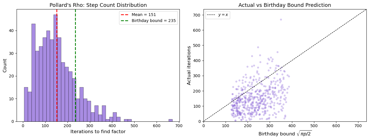
../_images/e34ba70195eac44babda1d9ad89dc5fc67ce9cfc727b694f76c28ac45b6a18eb.png

The scatter plot shows that the actual iteration count clusters around the birthday-bound prediction \(\sqrt{\pi p / 2}\), with the expected right-skewed distribution typical of coupon-collector-type processes.

27.14 Fermat’s Method: Speed vs Prime Gap#

We demonstrate how Fermat’s method performance depends critically on the gap \(|p - q|\) between the two factors.

../_images/ac32e3b48886143d36762b125b189bae02aaf90dd5afef0e6e0f50eac19ed297.png

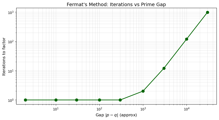
     Gap  Iterations
       2           1
         1
         1
         1
         1
         2
        12
       120
       983

Key Takeaway

The number of iterations grows roughly linearly with the gap \(|p - q|\), since Fermat’s method starts at \(\lceil\sqrt{n}\rceil\) and must increment \(a\) by approximately \(|p - q| / (2\sqrt{n})\) steps. For close primes, this is trivial; for well-separated primes, it becomes infeasible.

27.15 Algorithm#

Selection Guide

Scenario	Best Algorithm	Why
Small \(n\) (\(< 10^{12}\))	Trial division	Simple, fast enough
Medium \(n\) (\(< 10^{25}\))	Pollard’s rho	\(O(n^{1/4})\), no auxiliary storage
\(p-1\) is smooth	Pollard \(p-1\)	Exploits algebraic structure
\(p \approx q\) (close primes)	Fermat’s method	Very fast for small gap
Large \(n\) (\(> 10^{30}\))	Quadratic Sieve	Sub-exponential, practical
Very large \(n\) (\(> 10^{100}\))	GNFS	Asymptotically fastest known

In practice

Modern factoring software (e.g. YAFU, msieve, CADO-NFS) applies a cascade of methods: trial division up to \(10^6\), then ECM (elliptic curve method) to find factors up to ~35 digits, then QS or GNFS for the remaining cofactor.

27.16 Exercises#

Exercise 27.1#

Modify the trial_division function to return the complete prime factorisation of \(n\) as a dictionary {prime: exponent}. Test it on \(n = 2^{10} \times 3^5 \times 7^2 \times 13\).

Hint

Repeatedly divide \(n\) by each factor found until it no longer divides evenly. Count the number of times each factor divides. After exhausting all small factors, if the remaining cofactor is \(> 1\), it must be prime.

Exercise 27.2#

Implement a variant of Pollard’s rho that uses Brent’s improvement: instead of Floyd’s cycle detection, Brent’s method moves the “slow” pointer in powers of 2. Compare the average number of iterations with Floyd’s version on 100 random 10-digit composites.

Hint

In Brent’s variant, set \(y = x_0\), \(r = 1\), \(q = 1\). Let \(x\) advance \(r\) steps. Accumulate \(q = q \cdot |x - y| \bmod n\). Check \(\gcd(q, n)\) every \(r\) steps, then double \(r\) and set \(y = x\). This reduces the number of GCD computations and typically finds factors in about 25% fewer iterations.

Exercise 27.3#

The two-stage Pollard \(p-1\) method uses a second bound \(B_2 > B_1\): after the first stage with bound \(B_1\), check whether \(p - 1\) has exactly one prime factor between \(B_1\) and \(B_2\). Implement this and show it can factor \(n = 1000000007 \times 1000000009\) with \(B_1 = 100\) and \(B_2 = 50000\).

Hint

After the first stage, you have \(a = 2^M \bmod n\) where \(M = \text{lcm}(1,\ldots,B_1)\). In the second stage, for each prime \(q\) with \(B_1 < q \le B_2\), compute \(a^q \bmod n\) and check \(\gcd(a^q - 1, n)\). Use the fact that consecutive primes have small gaps to speed this up by precomputing \(a^{2k}\) for small \(k\).

Exercise 27.4#

Write a function factoring_race(n) that runs trial division, Pollard’s rho, and Fermat’s method concurrently (using iterative round-robin, not threads) and returns the factor found by whichever algorithm “wins” first. Test on several composites where different algorithms have the advantage.

Hint

Implement each algorithm as a generator that yields after each iteration. Then interleave them in a round-robin loop:

for alg in cycle([td_gen, rho_gen, fermat_gen]):
    result = next(alg)
    if result is not None:
        return result

This simulates concurrent execution without threading.

Exercise 27.5#

A Cunningham number is an integer of the form \(b^n \pm 1\). For \(b = 2\) and \(n = 64\), we have \(2^{64} - 1 = 18446744073709551615\).

Factor \(2^{64} - 1\) completely using your implemented algorithms.
Why is the \(p - 1\) method particularly effective here? (Hint: think about the algebraic structure of the factors.)
Factor \(2^{128} - 1\) and verify your result.

Hint

Use the algebraic factorisation \(2^{64} - 1 = (2^{32} - 1)(2^{32} + 1)\) and continue recursively. For factors of \(2^k - 1\) (Mersenne-type), every prime factor \(p\) satisfies \(p \equiv 1 \pmod{k}\), which means \(p - 1\) is divisible by \(k\) and is often smooth – making \(p - 1\) particularly effective.

27.17 Summary#

In this chapter we studied the major integer factoring algorithms, each exploiting a different mathematical property:

Trial division is the baseline: exhaustive, \(O(\sqrt{n})\), but always works.
Pollard’s rho uses the birthday paradox to achieve \(O(n^{1/4})\) expected time with negligible memory.
Pollard’s \(p-1\) targets primes \(p\) where \(p - 1\) is smooth, reminding us why safe-prime generation matters.
Fermat’s method is devastating when \(p \approx q\), enforcing the requirement that RSA primes be well-separated.
The Quadratic Sieve and GNFS are sub-exponential, with GNFS being the fastest known general algorithm at \(L_n[1/3, 1.923]\).

The practical security of RSA depends on choosing primes that resist all of these attacks simultaneously: large enough to defeat GNFS, with \(p - 1\) having a large prime factor, and \(|p - q|\) sufficiently large.

27.18 References#

Pollard, J.M. (1975). “A Monte Carlo method for factorization.” BIT Numerical Mathematics, 15(3), 331–334.
Pollard, J.M. (1974). “Theorems on factorization and primality testing.” Mathematical Proceedings of the Cambridge Philosophical Society, 76(3), 521–528.
Pomerance, C. (1996). “A tale of two sieves.” Notices of the AMS, 43(12), 1473–1485.
Lenstra, A.K. and Lenstra, H.W. Jr., eds. (1993). The Development of the Number Field Sieve. Lecture Notes in Mathematics 1554, Springer.
Crandall, R. and Pomerance, C. (2005). Prime Numbers: A Computational Perspective. 2nd edition, Springer.
Boudot, F. et al. (2020). “Factorization of RSA-250.” Cryptology ePrint Archive, Report 2020/697.
NIST SP 800-56B Rev. 2 (2019). “Recommendation for Pair-Wise Key Establishment Using Integer Factorization Cryptography.” Appendix B: requirements on RSA key generation.

Chapter 27: Integer Factoring Algorithms

Contents

Chapter 27: Integer Factoring Algorithms#

27.1 Historical Overview#

27.2 The Complexity Landscape#

27.3 Trial Division#

27.4 Pollard’s Rho Algorithm#

27.4.1 Visualising the Rho Trajectory#

27.5 Pollard’s \(p-1\) Method#

27.6 Fermat’s Factoring Method#

27.7 Quadratic Sieve – Conceptual Overview#

Core idea#

Complexity#

27.8 General Number Field Sieve (GNFS) – Conceptual Overview#

High-level steps#

Complexity#

27.9 Timing Comparison: Trial Division vs Pollard’s Rho vs \(p-1\)#

27.10 Experiment: \(p-1\) Success Rate vs Smoothness Bound#

27.11 Historical Factoring Records#

27.12 Experiment: Factoring Difficulty vs Number of Digits#

27.13 Pollard’s Rho: Step Count Histogram#

27.14 Fermat’s Method: Speed vs Prime Gap#

27.15 Algorithm#

27.16 Exercises#

Exercise 27.1#

Exercise 27.2#

Exercise 27.3#

Exercise 27.4#

Exercise 27.5#

27.17 Summary#

27.18 References#