
Chapter 32: Point Groups on Elliptic Curves (SageMath)#
Python Version Available
This notebook contains the SageMath implementation. A pure Python/NumPy version is available in Chapter 32: Point Groups on Elliptic Curves.
32.1 Introduction#
Every elliptic curve \(E\) over a finite field \(\mathbb{F}_p\) gives rise to a finite abelian group \(E(\mathbb{F}_p)\) consisting of all rational points together with the point at infinity \(\mathcal{O}\). Understanding the structure of this group is fundamental to elliptic curve cryptography: the security of protocols such as ECDH and ECDSA depends on \(E(\mathbb{F}_p)\) containing a large cyclic subgroup of prime order.
In this chapter we develop algorithms to:
Count the number of points on \(E(\mathbb{F}_p)\) (naive method, collision method, and overview of Schoof’s algorithm).
Determine the group structure: is the group cyclic, or a product of two cyclic groups?
Find generators of the group.
Visualise how group orders distribute relative to \(p + 1\).
All implementations use SageMath’s built-in elliptic curve machinery: EllipticCurve, GF(),
.order(), .abelian_group(), .gens(), and .division_polynomial(), which replace
hundreds of lines of manual Python arithmetic.
32.2 Background: Hasse’s Theorem and the Structure Theorem#
Theorem 32.1 (Hasse’s Theorem and Structure of Point Groups)
Let \(E: y^2 = x^3 + Ax + B\) be an elliptic curve over a finite field \(\mathbb{F}_p\). The set \(G = E(\mathbb{F}_p) = \{(x,y) \in \mathbb{F}_p^2 : y^2 = x^3 + Ax + B\} \cup \{\mathcal{O}\}\) has the following properties:
(Hasse’s theorem) There exists an integer \(a\) with \(|a| \le 2\sqrt{p}\) such that \(|E(\mathbb{F}_p)| = p + 1 - a\). The integer \(a\) is called the trace of Frobenius.
(Structure theorem) There exist positive integers \(n_1, n_2\) with \(n_2 \mid n_1\) and \(n_2 \mid (p - 1)\) such that
\[ E(\mathbb{F}_p) \cong \mathbb{Z}/n_1\mathbb{Z} \times \mathbb{Z}/n_2\mathbb{Z}.\]In particular, \(|E(\mathbb{F}_p)| = n_1 \cdot n_2\).
The group is cyclic (i.e., \(n_2 = 1\)) if and only if it is generated by a single point. In practice, most elliptic curves over \(\mathbb{F}_p\) have cyclic point groups.
Definition 32.2 (Group Structure Decomposition)
The decomposition \(E(\mathbb{F}_p) \cong \mathbb{Z}/n_1\mathbb{Z} \times \mathbb{Z}/n_2\mathbb{Z}\) with \(n_2 \mid n_1\) and \(n_2 \mid \gcd(n_1, p-1)\) is called the invariant factor decomposition of the point group. When \(n_2 = 1\), the group is cyclic of order \(n_1 = |E(\mathbb{F}_p)|\).
In these notes we will explore and compare the speed of several methods which establish the size of the point group.
32.3 Naive Point Counting#
A naive method for establishing the size requires solving several equations of the form \(y^2=x^3+Ax+B\), looping over values \(x\in\mathbb{F}_{p}\) and checking whether \(x^3+Ax+B\) is a square or not. In the case when \(x^3+Ax+B\) is a non-zero square we add \(2\) points to the count, namely \((x,y)\) and \((x,-y)\). If \(x^3+Ax+B\) is zero, then we add point \((x,0)\) only. Finally we add \(1\) to the counter for the point at infinity.
Complexity
This algorithm has complexity \(O(p \log p)\) (one modular exponentiation per \(x\)-value), which is exponential in \(\log p\). It is unusable for primes of cryptographic size.
def NaiveAlg(A,B,p):
    F=GF(p) #finite field structure
    if F(4*A^3+27*B^2)==0:
        print("For (A,B) = (%s,%s) this is not an elliptic curve (singularity)."%(A,B))
        return -1
    count=1
    for x in F:
        v=x*(x^2+A)+B
        if v.is_square(): #we will study this procedure next week
            if v==0:
                count+=1
            else:
                count+=2
    return count
NaiveAlg(1,2,11)
16
Timing the naive algorithm#
Let us see how the runtime scales as \(p\) grows. Since the algorithm is \(O(p)\), each tenfold increase in \(p\) should roughly multiply the runtime by 10.
%timeit NaiveAlg(11,13,19)
23.5 μs ± 480 ns per loop (mean ± std. dev. of 7 runs, 10,000 loops each)
%timeit NaiveAlg(12221,1333,193)
199 μs ± 2.13 μs per loop (mean ± std. dev. of 7 runs, 10,000 loops each)
%timeit NaiveAlg(12221,1333,613)
719 μs ± 8.09 μs per loop (mean ± std. dev. of 7 runs, 1,000 loops each)
(1919322393293).factor()
2729 * 703306117
%timeit NaiveAlg(12221,1333,3229)
3.87 ms ± 36.1 μs per loop (mean ± std. dev. of 7 runs, 100 loops each)
Primes()[1000]
7927
%timeit NaiveAlg(12221,1333,7927)
9.78 ms ± 211 μs per loop (mean ± std. dev. of 7 runs, 100 loops each)
Primes()[10000]
104743
%timeit NaiveAlg(12221,1333,104743)
131 ms ± 2.68 ms per loop (mean ± std. dev. of 7 runs, 10 loops each)
Comparison with SageMath’s built-in E.order()#
SageMath uses Schoof’s algorithm (and its Elkies–Atkin improvements) internally.
The built-in .order() method is polynomial-time in \(\log p\) and runs instantly
even for cryptographic-size primes.
# Compare: naive vs built-in for a moderate prime
p = 7927
E = EllipticCurve(GF(p), [12221, 1333])
print("Built-in E.order():", E.order())
print("Naive NaiveAlg:    ", NaiveAlg(12221, 1333, p))
Built-in E.order(): 8052
Naive NaiveAlg:     8052
# Built-in works instantly even for much larger primes
p_large = next_prime(10^20)
E_large = EllipticCurve(GF(p_large), [1, 3])
print(f"p = {p_large}")
print(f"|E(F_p)| = {E_large.order()}")
print(f"Trace of Frobenius a = {p_large + 1 - E_large.order()}")
p = 100000000000000000039
|E(F_p)| = 100000000009207625256
Trace of Frobenius a = -9207625216
32.4 Determining the Group Structure#
SageMath provides .abelian_group() and .gens() to determine the group structure
directly. Use P.order() to establish the order of any point on the curve.
To determine \(n_1\) and \(n_2\) manually, one can use the following strategy:
Compute \(N = |E(\mathbb{F}_p)|\) (via naive counting for small \(p\), or
.order()).The maximal order among all points equals \(n_1\) (the exponent of the group).
Then \(n_2 = N / n_1\).
Verify that \(n_2 \mid n_1\) and \(n_2 \mid (p - 1)\).
NaiveAlg(1,2,11)
16
This means on the elliptic curve \(y^2=x^3+x+2\) over \(\mathbb{F}_{11}\) we have \(|E(\mathbb{F}_{p})| = 16\).
Exercise: What is the structure of this group?
F=GF(11)
E=EllipticCurve([F(1),F(2)])
[P.order() for P in E]
[1, 4, 4, 8, 8, 8, 8, 2, 8, 8, 2, 4, 4, 8, 8, 2]
E.order()
16
E.abelian_group()
Additive abelian group isomorphic to Z/8 + Z/2 embedded in Abelian group of points on Elliptic Curve defined by y^2 = x^3 + x + 2 over Finite Field of size 11
So \(E(\mathbb{F}_{11}) \cong \mathbb{Z}/8\mathbb{Z} \times \mathbb{Z}/2\mathbb{Z}\).
This is a non-cyclic group.
Note that \(n_2 = 2\) divides \(n_1 = 8\) and \(n_2 = 2\) divides \(p - 1 = 10\), as required by the structure theorem.
Exercise: Find two points on the elliptic curve such that one has order 8 and the other has order 2.
# Find generators: SageMath provides them directly
G = E.abelian_group()
print("Generators:", G.gens())
print("Orders:    ", [g.order() for g in G.gens()])
Generators: ((6 : 2 : 1), (5 : 0 : 1))
Orders:     [8, 2]
# Another example: a cyclic group
EllipticCurve([GF(19)(7),5]).abelian_group()
Additive abelian group isomorphic to Z/15 embedded in Abelian group of points on Elliptic Curve defined by y^2 = x^3 + 7*x + 5 over Finite Field of size 19
Definition 32.3 (Torsion Subgroup)
For a positive integer \(m\), the \(m\)-torsion subgroup of \(E(\mathbb{F}_p)\) is
If \(\gcd(m, p) = 1\), then \(E[m] \cong \mathbb{Z}/m\mathbb{Z} \times \mathbb{Z}/m\mathbb{Z}\) when considered over the algebraic closure \(\overline{\mathbb{F}_p}\). Over \(\mathbb{F}_p\) itself, \(E[m]\) may be smaller – it is a subgroup of \(\mathbb{Z}/m\mathbb{Z} \times \mathbb{Z}/m\mathbb{Z}\).
The \(m\)-torsion subgroup plays a central role in Schoof’s algorithm: by computing the action of the Frobenius endomorphism on \(E[\ell]\) for small primes \(\ell\), one can determine \(a \bmod \ell\) and then reconstruct \(a\) via the Chinese Remainder Theorem.
32.5 Experiment: Group Structures for Various Curves and Primes#
Let us survey the group structure of \(E(\mathbb{F}_p)\) for several curves and primes,
using SageMath’s built-in abelian_group() method.
# Survey group structures for a range of curves
test_cases = [
    (1, 2, 11),
    (7, 5, 19),
    (1, 1, 19),
    (11, 3, 193),
    (12, 5, 271),
    (199, 272, 1013),
    (1, 3, 7927),
    (2, 7, 997),
    (3, 5, 1009),
    (5, 11, 2003),
]

print(f"{'Curve (A,B)':>14s}  {'p':>6s}  {'|E|':>6s}  {'Trace a':>8s}  {'Structure':>20s}  {'Cyclic':>7s}")
print("-" * 75)
for A, B, p in test_cases:
    F = GF(p)
    disc = F(4*A^3 + 27*B^2)
    if disc == 0:
        print(f"  ({int(A):>3d},{int(B):>3d})    {int(p):>6d}  -- singular --")
        continue
    E = EllipticCurve([F(A), F(B)])
    N = E.order()
    a_trace = p + 1 - N
    G = E.abelian_group()
    struct_str = str(G)
    invs = [i for i in G.invariants() if i > 1]
    is_cyc = "yes" if len(invs) <= 1 else "no"
    print(f"  ({int(A):>3d},{int(B):>3d})    {int(p):>6d}  {int(N):>6d}  {int(a_trace):>8d}  {struct_str:>20s}  {is_cyc:>7s}")
   Curve (A,B)       p     |E|   Trace a             Structure   Cyclic
---------------------------------------------------------------------------
  (  1,  2)        11      16        -4  Additive abelian group isomorphic to Z/8 + Z/2 embedded in Abelian group of points on Elliptic Curve defined by y^2 = x^3 + x + 2 over Finite Field of size 11       no
  (  7,  5)        19      15         5  Additive abelian group isomorphic to Z/15 embedded in Abelian group of points on Elliptic Curve defined by y^2 = x^3 + 7*x + 5 over Finite Field of size 19      yes
  (  1,  1)        19      21        -1  Additive abelian group isomorphic to Z/21 embedded in Abelian group of points on Elliptic Curve defined by y^2 = x^3 + x + 1 over Finite Field of size 19      yes
  ( 11,  3)       193     194         0  Additive abelian group isomorphic to Z/194 embedded in Abelian group of points on Elliptic Curve defined by y^2 = x^3 + 11*x + 3 over Finite Field of size 193      yes
  ( 12,  5)       271     289       -17  Additive abelian group isomorphic to Z/289 embedded in Abelian group of points on Elliptic Curve defined by y^2 = x^3 + 12*x + 5 over Finite Field of size 271      yes
  (199,272)      1013    1035       -21  Additive abelian group isomorphic to Z/1035 embedded in Abelian group of points on Elliptic Curve defined by y^2 = x^3 + 199*x + 272 over Finite Field of size 1013      yes
  (  1,  3)      7927    7925         3  Additive abelian group isomorphic to Z/7925 embedded in Abelian group of points on Elliptic Curve defined by y^2 = x^3 + x + 3 over Finite Field of size 7927      yes
  (  2,  7)       997    1045       -47  Additive abelian group isomorphic to Z/1045 embedded in Abelian group of points on Elliptic Curve defined by y^2 = x^3 + 2*x + 7 over Finite Field of size 997      yes
  (  3,  5)      1009    1023       -13  Additive abelian group isomorphic to Z/1023 embedded in Abelian group of points on Elliptic Curve defined by y^2 = x^3 + 3*x + 5 over Finite Field of size 1009      yes
  (  5, 11)      2003    1974        30  Additive abelian group isomorphic to Z/1974 embedded in Abelian group of points on Elliptic Curve defined by y^2 = x^3 + 5*x + 11 over Finite Field of size 2003      yes
Observation
Most curves in the table above are cyclic (\(n_2 = 1\)). The non-cyclic cases correspond to group orders that have a non-trivial common factor with \(p - 1\), and even then the group is often cyclic. Non-cyclic groups are the exception, not the rule.
32.6 Finding Generators#
Once we know the structure \(E(\mathbb{F}_p) \cong \mathbb{Z}/n_1\mathbb{Z} \times \mathbb{Z}/n_2\mathbb{Z}\), we need to find generators: a point \(P_1\) of order \(n_1\) and (if \(n_2 > 1\)) a point \(P_2\) of order \(n_2\) such that \(P_2 \notin \langle P_1 \rangle\).
SageMath provides .gens() directly through the abelian_group() method.
# E(F_11): non-cyclic example Z/8 x Z/2
F = GF(11)
E = EllipticCurve([F(1), F(2)])
G = E.abelian_group()
gens = G.gens()
print(f"Structure: {G}")
print(f"Generators: {gens}")
print(f"Orders: {[g.order() for g in gens]}")
print(f"Cyclic? {len([i for i in G.invariants() if i > 1]) <= 1}")
Structure: Additive abelian group isomorphic to Z/8 + Z/2 embedded in Abelian group of points on Elliptic Curve defined by y^2 = x^3 + x + 2 over Finite Field of size 11
Generators: ((6 : 2 : 1), (5 : 0 : 1))
Orders: [8, 2]
Cyclic? False
# E(F_19): cyclic example
F19 = GF(19)
E19 = EllipticCurve([F19(7), F19(5)])
G19 = E19.abelian_group()
gens19 = G19.gens()
print(f"Structure: {G19}")
print(f"Generator: {gens19}")
print(f"Order: {E19.order()}")
print(f"Cyclic? True")
Structure: Additive abelian group isomorphic to Z/15 embedded in Abelian group of points on Elliptic Curve defined by y^2 = x^3 + 7*x + 5 over Finite Field of size 19
Generator: ((18 : 4 : 1),)
Order: 15
Cyclic? True
Verification: enumerating generated points#
For small primes, we can verify our generators are correct by checking that every point on the curve can be expressed as \(a \cdot P_1 + b \cdot P_2\) for some integers \(a, b\).
# Verify generators for E(F_11)
F = GF(11)
E = EllipticCurve([F(1), F(2)])
G = E.abelian_group()
gens = G.gens()

# Convert abstract group generators to curve points
P1 = gens[0].element()
P2 = gens[1].element() if len(gens) > 1 else E(0)
n1 = gens[0].order()
n2 = gens[1].order() if len(gens) > 1 else 1

generated = set()
for a in range(n1):
    for b in range(n2):
        pt = a * P1 + b * P2
        generated.add(pt)

actual = set(E.points())
print(f"Generated {len(generated)} points, curve has {len(actual)} points")
print(f"Generators verified: {generated == actual}")
Generated 16 points, curve has 16 points
Generators verified: True
32.7 The Collision Method for Point Counting#
If the group \(E(\mathbb{F}_{p})\) is cyclic, then one can use the collision method to discover the structure and size of the group.
Namely, one chooses a random point \(P\) and computes its \(2^n P\) multiples until one hits a collision: two integers \(i\neq j\) such that \(2^i P = 2^j P\).
This means the order of the point \(P\) is a divisor of the number \(2^i-2^j\).
Knowing this, we can easily compute the exact order of the point by studying the divisors of the number \(2^i-2^j\). If the order \(\operatorname{ord}(P)\) of the point \(P\) lands in the interval \([p+1-2\sqrt{p},p+1+2\sqrt{p}]\) this means the point \(P\) is a generator of the group \(E(\mathbb{F}_{p})\) and the group is cyclic of order \(\operatorname{ord}(P)\).
p=Primes()[1000]
A=1
B=3
E=EllipticCurve([GF(p)(A),B])
#E.order().factor() #suppose we don't know that yet!
#E.abelian_group() #suppose we don't know that yet!
#collision method
def Collision(P,N):
    Pli={} # this is a collision set
    Q=P
    for i in range(0,N):
        if not (Q in Pli): #checking for collisions
            Pli[Q]=[i]
        else:
            print("Collision")
            return i,Pli[Q]
        Q=2*Q
    print("No collision found in the given range.")
    return -1
#P=E.random_point() #generate a random point by choosing x and varying it, with probability close to 100% in two steps we find a point
P=E([2643, 2059])
Collision(P,10000)
Collision
(1580, [0])
Usually the number \(2^i-2^j\) will be too large to completely factor.
Instead we look only for small prime factors of this number.
def SmallFactors(n,N):
    li=[]
    for p in Primes():
        if p>N:
            return li,n
        if n%p==0:
            li.append(p)
            while n%p==0:
                n/=p
SmallFactors(2^(1580)-1,10000)
([3, 5, 11, 31, 41, 317, 2687, 5531],
 8583473345751950624168340061080357313516254056686807398788251380929834539195812736002141774892386348847810084899666055728994413959110946072425945500101539586764658235777938094046153598097249374276409080234919894249115257764863511694617382296850515209541900513201266939069091096485012197422292044137883038884852354133219387566359473960926961338621430341241641934253182818715657954901045365382216075067434534241119423880332351266468532480011592357865980604331121)
5*317*P
(5411 : 7197 : 1)
5^2*P
(2695 : 7424 : 1)
5^2*317*P
(0 : 1 : 0)
p
7927
So the point \(P=(2643, 2059)\) on the elliptic curve \(E: y^2=x^3+x+3\) over the field \(\mathbb{F}_{p}\) with \(p=7927\) has order \(7925\).
From the Hasse theorem we obtain:
hasserange=[ceil(float(p+1-2*sqrt(p))),floor(float(p+1+2*sqrt(p)))]
hasserange
[7750, 8106]
So the number \(7925\) lands in the correct range.
Hence the point group is generated by the point \(P\) and is cyclic of the same order.
This means, every other point in the point group is a multiple of the point \(P\).
# Verify: all points on E are multiples of P
{Q for Q in E} == {k*P for k in range(7927)}
True
We can also verify using SageMath’s built-in methods:
# Cross-check with SageMath's built-in order computation
print(f"P.order() = {P.order()}")
print(f"E.order() = {E.order()}")
print(f"E.abelian_group() = {E.abelian_group()}")
P.order() = 7925
E.order() = 7925
E.abelian_group() = Additive abelian group isomorphic to Z/7925 embedded in Abelian group of points on Elliptic Curve defined by y^2 = x^3 + x + 3 over Finite Field of size 7927
Exercise 32.1: Collision method practice
Use collision method with
\((A,B)=(11,3)\) and \(p=193\)
\((A,B)=(12,5)\) and \(p=271\)
\((A,B)=(199,272)\) and \(p=1013\)
to find a generator for the group \(E(\mathbb{F}_{p})\).
Hint
Start by finding a point: try \(x = 0, 1, 2, \ldots\) until \(x^3 + Ax + B\) is a quadratic
residue mod \(p\), or use E.random_point(). Then apply Collision and SmallFactors. The Hasse
interval is \([p + 1 - 2\lfloor\sqrt{p}\rfloor,\, p + 1 + 2\lfloor\sqrt{p}\rfloor]\).
32.8 Baby Step-Giant Step#
The baby step-giant step method is a meet-in-the-middle approach for computing the order of a point (or equivalently the group order when the group is cyclic). Given a point \(P\) and the Hasse interval \([p+1-2\sqrt{p}, p+1+2\sqrt{p}]\), one computes:
Baby steps: \(jP\) for \(j = 0, 1, \ldots, m\) where \(m = \lceil p^{1/4} \rceil\).
Giant steps: \((p+1)P + k(2m)P\) for \(k = -m, \ldots, m\).
A match between a baby step and a giant step reveals a multiple of the order. This method has time and space complexity \(O(p^{1/4})\).
In SageMath, P.order() uses similar (and faster) techniques internally.
def BSGS_order(E, P):
    """Baby step-giant step method to find the order of point P on curve E over F_p.
    Uses the Hasse bound to limit the search range."""
    p = E.base_field().order()
    m = ceil(p^(ZZ(1)/4))  # step size

    # Baby steps: compute jP for j = 0, 1, ..., 2m
    baby = {}
    R = E(0)  # identity
    for j in range(2*m + 1):
        baby[R] = j
        R = R + P

    # Giant step size
    G = (2*m)*P

    # Start at (p+1)*P and step by G
    Q = (p + 1)*P

    for k in range(-m, m + 1):
        R = Q + k*G
        if R in baby:
            # Found match: (p+1 + 2mk)P = jP
            # So (p+1 + 2mk - j)P = O
            candidate = p + 1 + 2*m*k - baby[R]
            if candidate > 0:
                # Refine: find exact order by dividing out prime factors
                order = candidate
                for (q, _) in factor(candidate):
                    while order % q == 0 and (order // q)*P == E(0):
                        order = order // q
                return order
    return None

# Test
p = Primes()[1000]
E = EllipticCurve(GF(p), [1, 3])
P = E([2643, 2059])
order_bsgs = BSGS_order(E, P)
print(f"BSGS order of P: {order_bsgs}")
print(f"Built-in P.order(): {P.order()}")
print(f"Match: {order_bsgs == P.order()}")
BSGS order of P: 7925
Built-in P.order(): 7925
Match: True
32.9 Schoof’s Method#
The naive counting method is \(O(p)\), which is exponential in \(\log p\). For cryptographic primes (\(p \approx 2^{256}\)), this is completely infeasible.
Schoof’s algorithm (1985) computes \(|E(\mathbb{F}_p)|\) in polynomial time \(O(\log^8 p)\) (or better with the Schoof-Elkies-Atkin improvements).
The key idea:
The Frobenius endomorphism \(\phi: (x, y) \mapsto (x^p, y^p)\) satisfies \(\phi^2 - a\phi + p = 0\) on \(E\), where \(a = p + 1 - |E(\mathbb{F}_p)|\).
For each small prime \(\ell\), restrict to the \(\ell\)-torsion subgroup \(E[\ell]\) and compute \(a \bmod \ell\) by checking which value makes the characteristic equation hold.
Use the Chinese Remainder Theorem to reconstruct \(a\) from its residues modulo \(\ell_1, \ell_2, \ldots, \ell_k\), where \(\prod \ell_i > 4\sqrt{p}\).
In this method we use \(\ell\)-torsion points in \(E(\mathbb{F}_{p})\) to reconstruct the information about \(a \pmod{\ell}\) where \(a\) is the unique integer such that \(|E(\mathbb{F}_p)| = p+1-a\). Application of the Chinese Remainder Theorem for sufficiently many reductions modulo \(\ell\) will reconstruct the integer \(a\) uniquely. Notice that the integer \(a\) has absolute value at most \(2\sqrt{p}\) and might be negative.
Example: \(E: y^2=x^3+x+1\) over \(\mathbb{F}_{19}\)#
Compute the group size of \(E(\mathbb{F}_p)\) for \(E: y^2=x^3+x+1\), \(p=19\).
p=19
E=EllipticCurve(GF(p),[1,1])
E.order() #Schoof
21
Step 1: Find 3-torsion points using the division polynomial#
E.division_polynomial(3).factor()
(3) * (x + 17) * (x^3 + 2*x^2 + 6*x + 16)
# Frobenius action on a 3-torsion point via quotient ring
R.<x,y>=PolynomialRing(GF(p),2)

I=R.ideal([x+17,y^2-(x^3 + x + 1)])
Q=R.quotient_ring(I)


def Frob(x,y):
    return Q(x^p),Q(y^p)


Frob(x,y)
(2, ybar)
# Note: In some SageMath versions, change_ring with a quotient ring
# that has a multi-generator ideal causes a ValueError in normalize_coordinates.
# We use the Frob function from the previous cell instead.
try:
    E.change_ring(Q)([x^p,y^p])
except (ValueError, TypeError) as e:
    print(f"E.change_ring(Q)([x^p,y^p]) raised: {e}")
    print("Using Frob function instead:")
    print(Frob(x,y))
E.change_ring(Q)([x^p,y^p]) raised: too many values to unpack (expected 1)
Using Frob function instead:
(2, ybar)
I.groebner_basis() #solutions
[y^2 + 8, x - 2]
3*E([2,7])
(0 : 1 : 0)
P1=E([2,7])
Step 2: Determine \(a \bmod 3\)#
#Hasse range for a; |E(F_p)| = p+1 - a
[-2*sqrt(p).n(),2*sqrt(p).n()]
[-8.71779788708135, 8.71779788708135]
#trace a modulo 3 is unique!
for a in range(-8,9):
    if (P1+a*P1+p*P1).is_zero():
        print(a%3)
1
1
1
1
1
1
Step 3: Find more torsion primes#
We need the product of our primes \(\ell\) to exceed \(4\sqrt{p}\):
#we look for prime numbers such that, their product is larger than...
4*sqrt(p).n()
17.4355957741627
#no 5-torsion points
E.division_polynomial(5).factor()
(5) * (x^2 + x + 10) * (x^10 + 18*x^9 + 11*x^8 + 18*x^7 + 3*x^6 + 17*x^5 + 16*x^4 + 13*x^3 + 7*x^2 + 2*x + 3)
#we have some 7-torsion points
E.division_polynomial(7).factor()
(7) * (x + 4) * (x + 5) * (x + 9) * (x^3 + 7*x^2 + 15*x + 8) * (x^6 + 8*x^5 + 6*x^4 + 15*x^3 + 8*x + 17) * (x^6 + 12*x^5 + 10*x^4 + 4*x^3 + 11*x^2 + 4*x + 13) * (x^6 + 12*x^5 + 18*x^4 + 18*x^3 + 13*x^2 + 17*x + 4)
#point check
GF(p)(7^3+7+1).sqrt()
3
P2=E([15,3])
#order of P2
7*P2
(0 : 1 : 0)
Step 4: Determine \(a \bmod 7\)#
for a in range(-8,9):
    if (P2+a*P2+p*P2).is_zero():
        print(a%7)
1
1
1
Step 5: Reconstruct \(a\) via CRT#
#reconstruct a modulo 21
CRT([-1,-1],[3,7])
20
20-3*7
-1
#order of E(F_p)
p+1-(-1)
21
Important caveat
The demonstration above illustrates the CRT-based reconstruction principle of Schoof’s
algorithm. The real algorithm works with division polynomials in the polynomial ring
\(\mathbb{F}_p[x]\) to compute the action of the Frobenius on \(E[\ell]\) without enumerating
individual \(\ell\)-torsion points. This is what makes it polynomial-time.
SageMath’s E.order() uses the full Schoof-Elkies-Atkin algorithm internally.
Example: Schoof’s method for \(p = 1229\)#
Exercise 32.2: CRT and Schoof’s principle
Take \(p=1229\) and \((A,B)=(1,1)\). Find the order of \(E(\mathbb{F}_{p})\) using Schoof’s method.
Hint
For \(p = 1229\), the Hasse bound gives \(|a| \le 2\sqrt{1229} \approx 70.1\). You need \(\prod \ell_i > 4\sqrt{p} \approx 140.2\), and indeed \(3 \times 47 = 141 > 140.2\). To find an \(\ell\)-torsion point, find any point \(Q\) and compute \((|E|/\ell) \cdot Q\); if \(\ell \mid |E|\), this gives an \(\ell\)-torsion point (possibly \(\mathcal{O}\), in which case try another \(Q\)).
p=1229
E=EllipticCurve(GF(p),[1,1])
E.order() #Schoof
1269
#computations

P1=E([1076,97])
assert (3*P1).is_zero()
P2=E([0,1])
assert (47*P2).is_zero()
#abs(a) is less than..
2*sqrt(p).n()
70.1141925718324
for a in range(-70,71):
    if (P1+a*P1+p*P1).is_zero():
        print(a%3)
0
0
0
0
0
0
0
0
0
0
0
0
0
0
0
0
0
0
0
0
0
0
0
0
0
0
0
0
0
0
0
0
0
0
0
0
0
0
0
0
0
0
0
0
0
0
0
for a in range(-70,71):
    if (P2+a*P2+p*P2).is_zero():
        print(a%47)
39
39
39
#size of the interval [p+1-2*sqrt(p),p+1+2*sqrt(p)]
4*sqrt(p).n()
140.228385143665
#Chinese Remainder Theorem reconstruction of a from its reductions modulo 3 and 47
CRT([0,-39],[3,47])
102
M=3*47
M
141
#value of a
102-M
-39
#point group size of E(F_p)
(p+1)-(-39)
1269
32.10 Experiment: Distribution of Group Orders (Hasse Histogram)#
Hasse’s theorem tells us \(|E(\mathbb{F}_p)| \in [p + 1 - 2\sqrt{p},\; p + 1 + 2\sqrt{p}]\). Let us fix a prime \(p\) and vary the curve parameters \((A, B)\) to see how the group order distributes within this interval.
# SageMath provides built-in plotting
# SageMath provides built-in numerical tools

p = 499  # a moderate prime
orders = []

F = GF(p)
for A in range(1, p):
    for B in range(1, min(p, 50)):  # sample B values to keep runtime manageable
        disc = F(4*A^3 + 27*B^2)
        if disc == 0:
            continue
        E = EllipticCurve([F(A), F(B)])
        orders.append(E.order())

hasse_low = int(p + 1 - 2*isqrt(p)) - 2
hasse_high = int(p + 1 + 2*isqrt(p)) + 2

# Build histogram data manually for SageMath bar_chart
from collections import Counter
order_freq = Counter(orders)
bin_range = range(hasse_low, hasse_high + 1)
hist_data = [order_freq.get(v, 0) for v in bin_range]
chart = bar_chart(hist_data, color='steelblue')
# Add vertical lines as annotations
center_idx = p + 1 - hasse_low
chart += line([(center_idx, 0), (center_idx, max(hist_data))], color='red', linestyle='--', thickness=2)
show(chart, figsize=[10, 5],
     title=f'Distribution of group orders for p = {p}')

print(f"\nSampled {len(orders)} curves over F_{p}")
print(f"Order range: [{min(orders)}, {max(orders)}]")
print(f"Hasse bounds: [{int(p + 1 - 2*isqrt(p))}, {int(p + 1 + 2*isqrt(p))}]")
print(f"Mean order: {float(sum(orders)/len(orders)):.1f}  (p+1 = {p+1})")
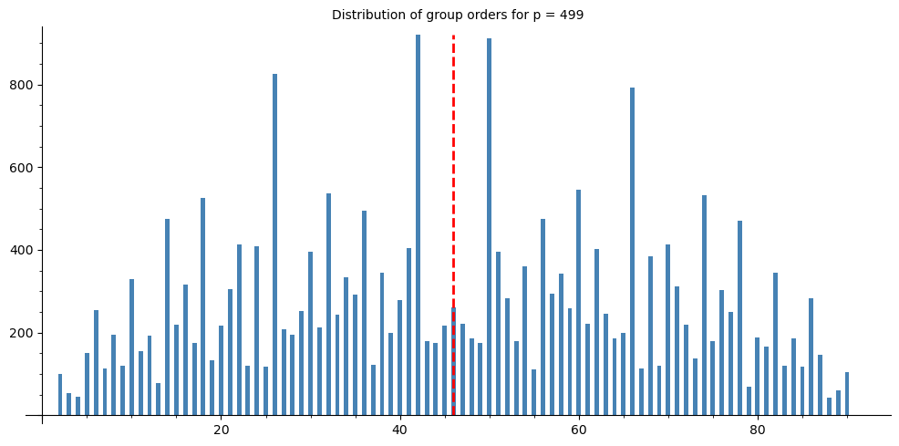
Sampled 24342 curves over F_499
Order range: [456, 544]
Hasse bounds: [456, 544]
Mean order: 500.1  (p+1 = 500)
Observation
The distribution of \(|E(\mathbb{F}_p)|\) is concentrated around \(p + 1\) and has a characteristic semicircular shape (related to the Sato-Tate distribution for the normalised trace \(a / (2\sqrt{p})\)). The histogram above illustrates this directly: most group orders cluster near \(p + 1\).
32.11 Experiment: Cyclic vs Non-Cyclic Groups#
How often is \(E(\mathbb{F}_p)\) cyclic? We survey many random curves for a fixed prime.
# SageMath provides built-in plotting
# SageMath provides built-in numerical tools

def survey_cyclic_sage(p, num_curves=500, seed=42):
    """Survey random curves over F_p and report cyclic vs non-cyclic counts."""
    set_random_seed(seed)
    F = GF(p)
    cyclic_count = 0
    noncyclic_count = 0
    noncyclic_examples = []

    attempts = 0
    while cyclic_count + noncyclic_count < num_curves and attempts < 5 * num_curves:
        attempts += 1
        A = F.random_element()
        B = F.random_element()
        if F(4*A^3 + 27*B^2) == 0:
            continue
        E = EllipticCurve([A, B])
        G = E.abelian_group()
        invs = [i for i in G.invariants() if i > 1]
        if len(invs) <= 1:
            cyclic_count += 1
        else:
            noncyclic_count += 1
            if len(noncyclic_examples) < 5:
                noncyclic_examples.append((int(A), int(B), E.order(), G))

    return cyclic_count, noncyclic_count, noncyclic_examples


# Survey for several primes
primes_survey = [101, 199, 307, 499, 701]
results = []

print(f"{'p':>6s}  {'Curves':>7s}  {'Cyclic':>7s}  {'Non-cyc':>8s}  {'% Cyclic':>9s}")
print("-" * 45)
for p in primes_survey:
    cyc, ncyc, examples = survey_cyclic_sage(p, num_curves=300)
    total = cyc + ncyc
    pct = 100 * cyc / total if total > 0 else 0
    results.append((p, cyc, ncyc, pct))
    print(f"{int(p):>6d}  {int(total):>7d}  {int(cyc):>7d}  {int(ncyc):>8d}  {float(pct):>8.1f}%")
    if examples:
        print(f"         Non-cyclic examples: {examples[:2]}")
     p   Curves   Cyclic   Non-cyc   % Cyclic
---------------------------------------------
   101      300      253        47      84.3%
         Non-cyclic examples: [(46, 16, 96, Additive abelian group isomorphic to Z/24 + Z/4 embedded in Abelian group of points on Elliptic Curve defined by y^2 = x^3 + 46*x + 16 over Finite Field of size 101), (69, 54, 112, Additive abelian group isomorphic to Z/56 + Z/2 embedded in Abelian group of points on Elliptic Curve defined by y^2 = x^3 + 69*x + 54 over Finite Field of size 101)]
   199      300      247        53      82.3%
         Non-cyclic examples: [(59, 101, 220, Additive abelian group isomorphic to Z/110 + Z/2 embedded in Abelian group of points on Elliptic Curve defined by y^2 = x^3 + 59*x + 101 over Finite Field of size 199), (190, 49, 216, Additive abelian group isomorphic to Z/108 + Z/2 embedded in Abelian group of points on Elliptic Curve defined by y^2 = x^3 + 190*x + 49 over Finite Field of size 199)]
   307      300      241        59      80.3%
         Non-cyclic examples: [(80, 28, 324, Additive abelian group isomorphic to Z/108 + Z/3 embedded in Abelian group of points on Elliptic Curve defined by y^2 = x^3 + 80*x + 28 over Finite Field of size 307), (215, 216, 300, Additive abelian group isomorphic to Z/150 + Z/2 embedded in Abelian group of points on Elliptic Curve defined by y^2 = x^3 + 215*x + 216 over Finite Field of size 307)]
   499      300      234        66      78.0%
         Non-cyclic examples: [(187, 67, 520, Additive abelian group isomorphic to Z/260 + Z/2 embedded in Abelian group of points on Elliptic Curve defined by y^2 = x^3 + 187*x + 67 over Finite Field of size 499), (461, 119, 480, Additive abelian group isomorphic to Z/240 + Z/2 embedded in Abelian group of points on Elliptic Curve defined by y^2 = x^3 + 461*x + 119 over Finite Field of size 499)]
   701      300      244        56      81.3%
         Non-cyclic examples: [(98, 389, 656, Additive abelian group isomorphic to Z/328 + Z/2 embedded in Abelian group of points on Elliptic Curve defined by y^2 = x^3 + 98*x + 389 over Finite Field of size 701), (538, 552, 672, Additive abelian group isomorphic to Z/168 + Z/4 embedded in Abelian group of points on Elliptic Curve defined by y^2 = x^3 + 538*x + 552 over Finite Field of size 701)]
# SageMath provides built-in plotting

# Bar chart: cyclic vs non-cyclic
primes_labels = [str(r[0]) for r in results]
cyc_counts = [r[1] for r in results]
ncyc_counts = [r[2] for r in results]

# Display as side-by-side bars using SageMath
chart_cyc = bar_chart(cyc_counts, color='steelblue', width=0.4)
chart_ncyc = bar_chart(ncyc_counts, color='salmon', width=0.4)
show(chart_cyc + chart_ncyc, title='Cyclic (blue) vs Non-Cyclic (red) Point Groups',
     figsize=[8, 5])

# Also show percentages
for i_v, (c, n) in enumerate(zip(cyc_counts, ncyc_counts)):
    total = c + n
    print(f"p={primes_labels[i_v]}: {float(100*c/total):.0f}% cyclic")
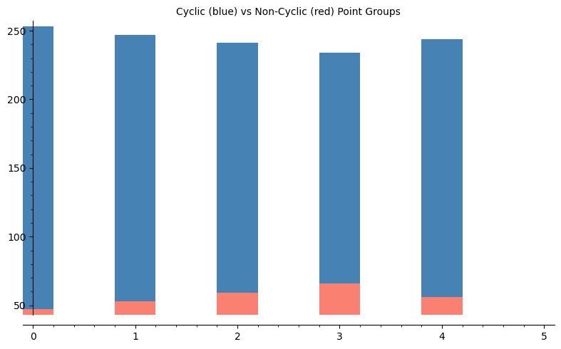
p=101: 84% cyclic
p=199: 82% cyclic
p=307: 80% cyclic
p=499: 78% cyclic
p=701: 81% cyclic
Observation
The vast majority of elliptic curves over \(\mathbb{F}_p\) have cyclic point groups. Heuristically, the probability that a random curve has non-cyclic group is roughly \(O(1/p)\), so as \(p\) grows, non-cyclic groups become extremely rare. This is good news for cryptography: randomly chosen curves almost always yield the cyclic groups needed for ECDLP-based protocols.
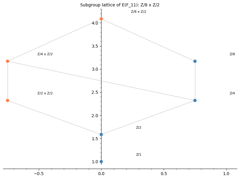
32.12 Visualising the Subgroup Lattice#
The subgroup lattice of a finite abelian group shows the inclusion relationships between all subgroups. For a cyclic group \(\mathbb{Z}/n\mathbb{Z}\), the subgroup lattice is isomorphic to the divisor lattice of \(n\). For \(\mathbb{Z}/n_1 \times \mathbb{Z}/n_2\), the structure is richer.
# SageMath provides built-in plotting

def divisors_list(n):
    """Return sorted list of divisors of n."""
    return sorted(Integer(n).divisors())


def subgroup_orders(n1, n2):
    """Compute all possible subgroup orders for Z/n1 x Z/n2.
    A subgroup of Z/n1 x Z/n2 has the form Z/d1 x Z/d2 where d1 | n1, d2 | n2, d2 | d1.
    Returns list of (d1, d2) pairs and the total order d1*d2."""
    subgroups = []
    for d1 in divisors_list(n1):
        for d2 in divisors_list(n2):
            if d2 <= d1 and d1 % d2 == 0:
                subgroups.append((d1, d2, d1 * d2))
    return subgroups


def plot_subgroup_lattice(n1, n2, title_str=""):
    """Plot the subgroup lattice of Z/n1 x Z/n2 using SageMath graphics."""
    subs = subgroup_orders(n1, n2)

    # Group by total order for y-position
    order_to_subs = {}
    for d1, d2, total in subs:
        order_to_subs.setdefault(total, []).append((d1, d2))

    sorted_orders = sorted(order_to_subs.keys())
    y_map = {}
    for i_o, order in enumerate(sorted_orders):
        y_map[order] = float(log(order + 1, 2))

    positions = {}
    for order in sorted_orders:
        group_list = order_to_subs[order]
        n_at_level = len(group_list)
        for j, (d1, d2) in enumerate(group_list):
            x_pos = (j - (n_at_level - 1) / 2) * 1.5
            y_pos = y_map[order]
            positions[(d1, d2)] = (x_pos, y_pos)

    # Determine Hasse edges (covers)
    edges = []
    for idx_a, (d1a, d2a, ta) in enumerate(subs):
        for idx_b, (d1b, d2b, tb) in enumerate(subs):
            if ta < tb and d1b % d1a == 0 and d2b % d2a == 0:
                is_cover = True
                for d1c, d2c, tc in subs:
                    if ta < tc < tb and d1c % d1a == 0 and d2c % d2a == 0 and d1b % d1c == 0 and d2b % d2c == 0:
                        is_cover = False
                        break
                if is_cover:
                    edges.append(((d1a, d2a), (d1b, d2b)))

    G = Graphics()

    for (a_node, b_node) in edges:
        xa, ya = positions[a_node]
        xb, yb = positions[b_node]
        G += line([(xa, ya), (xb, yb)], color='gray', alpha=0.5, thickness=0.8)

    for (d1, d2), (x_coord, y_coord) in positions.items():
        if d2 == 1:
            label = f"Z/{d1}"
            color = 'steelblue'
        else:
            label = f"Z/{d1} x Z/{d2}"
            color = 'coral'
        G += point2d([(x_coord, y_coord)], color=color, size=60, zorder=5)
        G += text(label, (x_coord + 0.3, y_coord + 0.15), fontsize=8, color='black')

    show(G, title=title_str, figsize=[8, 6], axes=True)


# Example 1: Z/8 x Z/2 (non-cyclic, our E(F_11) example)
plot_subgroup_lattice(8, 2,
    title_str='Subgroup lattice of E(F_11): Z/8 x Z/2')
# SageMath provides built-in plotting

# Example 2: Z/15 (cyclic, our E(F_19) example)
plot_subgroup_lattice(15, 1,
    title_str='Subgroup lattice of E(F_19): Z/15 (cyclic)')
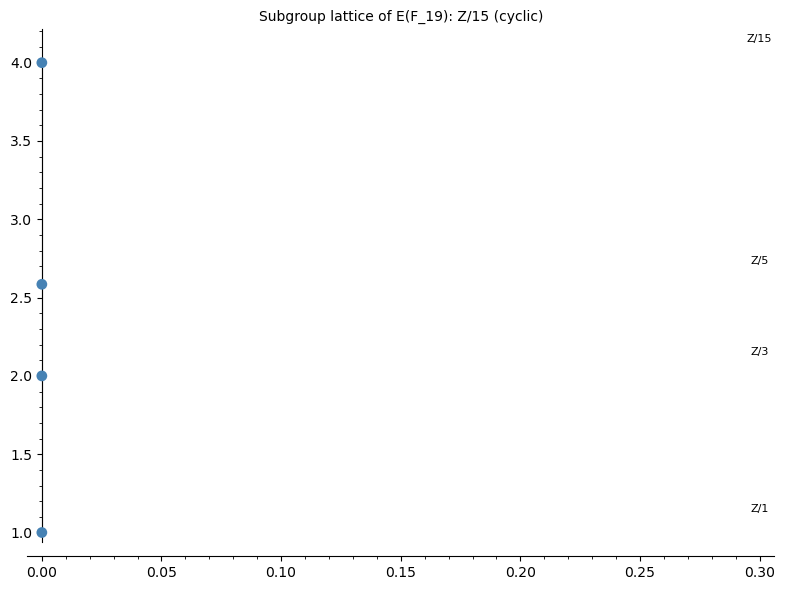
Comparing lattices
Notice that the lattice of \(\mathbb{Z}/8 \times \mathbb{Z}/2\) is wider than that of \(\mathbb{Z}/15\): at each level, there can be multiple subgroups of the same order. For the cyclic group \(\mathbb{Z}/15\), each divisor of 15 gives exactly one subgroup. This structural difference has consequences for cryptography: in a non-cyclic group, the discrete logarithm problem can potentially be decomposed into easier subproblems.
32.13 Sato-Tate Distribution: The Trace of Frobenius#
The Sato-Tate conjecture (now a theorem, proved by Taylor et al. in 2011 for non-CM curves over \(\mathbb{Q}\)) predicts that the normalised trace \(\theta = \arccos(a / (2\sqrt{p}))\) is distributed according to the density \(\frac{2}{\pi} \sin^2(\theta)\) on \([0, \pi]\).
Let us visualise this by computing the trace for many random curves.
# SageMath provides built-in plotting

p = 997
F = GF(p)
traces = []
set_random_seed(0)

for _ in range(3000):
    A = F.random_element()
    B = F.random_element()
    if F(4*A^3 + 27*B^2) == 0:
        continue
    E = EllipticCurve([A, B])
    N = E.order()
    a_val = p + 1 - N
    # Normalise: theta = arccos(a / (2*sqrt(p)))
    normalised = float(a_val) / (2 * float(sqrt(p)))
    if -1 <= normalised <= 1:
        theta = float(arccos(normalised))
        traces.append(theta)

# Build histogram data
from collections import Counter
n_bins = 50
bin_width = float(pi) / n_bins
hist_counts = [0] * n_bins
for th in traces:
    b = int(th / bin_width)
    if b >= n_bins:
        b = n_bins - 1
    hist_counts[b] += 1
# Normalize to density
total = len(traces)
hist_density = [c / (total * bin_width) for c in hist_counts]

# SageMath bar chart for histogram
chart = bar_chart(hist_density, color='steelblue', width=1.0)

# Overlay theoretical Sato-Tate density
theta_pts = [(float(t), (2 / float(pi)) * float(sin(t))^2)
             for t in srange(0.01, float(pi), 0.01)]
# Scale x-axis: bar_chart uses integer indices, so scale theta_pts
theta_scaled = [(t[0] / bin_width, t[1]) for t in theta_pts]
curve_plot = list_plot(theta_scaled, plotjoined=True, color='red', thickness=2)

show(chart + curve_plot, title=f'Sato-Tate distribution for p = {p}',
     figsize=[9, 5])

print(f"Computed traces for {len(traces)} curves over F_{p}")
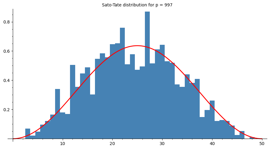
Computed traces for 2998 curves over F_997
32.14 Exercises#
Exercise 32.3: Point orders and cyclic detection
Consider the curve \(E: y^2 = x^3 + 11x + 3\) over \(\mathbb{F}_{193}\).
(a) Compute \(|E(\mathbb{F}_{193})|\) using E.order().
(b) Find a point \(P\) on \(E\) and compute its order using P.order().
(c) Is \(E(\mathbb{F}_{193})\) cyclic? Use E.abelian_group() to determine the structure.
If cyclic, find a generator. If not, find generators \(P_1, P_2\) for the two cyclic factors.
Hint
The group order should be close to \(p + 1 = 194\). For part (c), use E.abelian_group()
and .gens() to read off the structure and generators directly.
Exercise 32.4: Non-cyclic group construction
Find an elliptic curve \(E\) over \(\mathbb{F}_p\) (for some small prime \(p < 100\)) such that \(E(\mathbb{F}_p)\) is not cyclic, i.e., \(E(\mathbb{F}_p) \cong \mathbb{Z}/n_1 \times \mathbb{Z}/n_2\) with \(n_2 > 1\).
(a) Find such a curve by systematic search using EllipticCurve and abelian_group().
(b) Verify that \(n_2 \mid n_1\) and \(n_2 \mid (p - 1)\).
(c) Explain why the condition \(n_2 \mid (p - 1)\) is necessary.
Hint
Try \(p = 11\) and test various \((A, B)\) pairs. The curve \(y^2 = x^3 + x + 2\) over \(\mathbb{F}_{11}\) is a known non-cyclic example with structure \(\mathbb{Z}/8 \times \mathbb{Z}/2\). Note \(n_2 = 2\) divides \(p - 1 = 10\).
Exercise 32.5: Subgroup lattice exploration
(a) Draw (by hand or using code) the subgroup lattice for \(\mathbb{Z}/12\). How many subgroups are there?
(b) Draw the subgroup lattice for \(\mathbb{Z}/6 \times \mathbb{Z}/2\). Compare it with the lattice for \(\mathbb{Z}/12\) – they have the same order (12) but different structures.
(c) For a group \(\mathbb{Z}/n_1 \times \mathbb{Z}/n_2\) with \(n_2 \mid n_1\), prove that the number of subgroups is at least the number of divisors of \(n_1 \cdot n_2\). When does equality hold?
Hint
For part (a), \(\mathbb{Z}/12\) has subgroups of orders \(1, 2, 3, 4, 6, 12\) (one for each divisor). For part (b), \(\mathbb{Z}/6 \times \mathbb{Z}/2\) has additional subgroups beyond those of \(\mathbb{Z}/12\): for example, it has three subgroups of order 2 (generated by \((3, 0)\), \((0, 1)\), and \((3, 1)\)). Equality in (c) holds when the group is cyclic (\(n_2 = 1\)).
32.15 Summary#
In this chapter we studied the algebraic structure of the point group \(E(\mathbb{F}_p)\):
Hasse’s theorem bounds \(|E(\mathbb{F}_p)|\) in the interval \([p + 1 - 2\sqrt{p},\, p + 1 + 2\sqrt{p}]\).
The structure theorem tells us \(E(\mathbb{F}_p) \cong \mathbb{Z}/n_1 \times \mathbb{Z}/n_2\) with \(n_2 \mid n_1\) and \(n_2 \mid (p - 1)\).
Naive counting is \(O(p)\) and only feasible for small primes.
The collision method discovers the group order via repeated doublings and collision detection.
Baby step-giant step finds the order in \(O(p^{1/4})\) time.
Schoof’s algorithm computes \(|E(\mathbb{F}_p)|\) in polynomial time \(O(\log^8 p)\) by determining the trace of Frobenius modulo small primes and applying the CRT. SageMath’s
E.order()implements this internally.Most curves are cyclic: the probability of a random curve having a non-cyclic group is \(O(1/p)\), making cyclic groups overwhelmingly dominant for large primes.
The Sato-Tate distribution describes how the trace of Frobenius distributes across random curves: the normalised angle follows a \(\frac{2}{\pi}\sin^2(\theta)\) density.
These results underpin the selection of elliptic curves for cryptographic applications. In the next chapter, we will use this theory to set up the Elliptic Curve Discrete Logarithm Problem (ECDLP) and study its hardness.
32.16 References#
Hasse, H. (1936). Zur Theorie der abstrakten elliptischen Funktionenk”orper. Journal f”ur die reine und angewandte Mathematik, 175, 193–208.
Schoof, R. (1985). Elliptic curves over finite fields and the computation of square roots mod \(p\). Mathematics of Computation, 44(170), 483–494.
Silverman, J.H. (2009). The Arithmetic of Elliptic Curves, 2nd edition. Springer GTM 106.
Washington, L.C. (2008). Elliptic Curves: Number Theory and Cryptography, 2nd edition. Chapman & Hall/CRC.
Taylor, R. (2008). Automorphy for some \(l\)-adic lifts of automorphic mod \(l\) Galois representations, II. Publ. Math. IHES, 108, 183–239. (Part of the Sato-Tate proof.)
Blake, I.F., Seroussi, G., Smart, N.P. (1999). Elliptic Curves in Cryptography. Cambridge University Press.