
Chapter 34 — Gröbner Bases and Algebraic Foundations#
“Every ideal in a polynomial ring over a field has a finite generating set — a Gröbner basis — that makes membership decidable.” — Bruno Buchberger, 1965
In this chapter we introduce Gröbner bases and their computation via Buchberger’s algorithm, focusing on polynomial systems over \(\mathrm{GF}(2)\) relevant to algebraic cryptanalysis.
34.1 Historical Context#
Bruno Buchberger introduced Gröbner bases in his 1965 PhD thesis at the University of Innsbruck, naming them after his advisor Wolfgang Gröbner. The algorithm provides a systematic way to solve systems of polynomial equations — a generalization of Gaussian elimination from linear to nonlinear systems.
In the early 2000s, Nicolas Courtois and Josef Pieprzyk proposed using Gröbner bases to attack block ciphers algebraically. Their XSL attack (2002) aimed to express AES as a system of quadratic equations over \(\mathrm{GF}(2)\) and solve them. While the attack hasn’t broken AES in practice, it spurred significant research in algebraic cryptanalysis.
Tip
In the Boolean polynomial ring \(\mathrm{GF}(2)[x_1,\ldots,x_n]/\langle x_i^2 + x_i : i=1,\ldots,n\rangle\), every variable satisfies \(x_i^2 = x_i\) (since we quotient by the field equations). This is the natural algebraic setting for modeling Boolean circuits. Working in this quotient ring, we can always reduce any polynomial to multilinear form (degree at most 1 in each variable), which fundamentally limits the complexity of the polynomial system.
34.2 Formal Definitions#
Definition 34.1 — Polynomial Ideal
An ideal \(I\) in a polynomial ring \(K[x_1, \ldots, x_n]\) over a field \(K\) is a subset closed under addition and multiplication by ring elements:
In cryptographic applications, we typically work over \(\mathrm{GF}(2)\).
Definition 34.2 — Monomial Ordering
A monomial ordering \(\prec\) on \(\{x_1^{a_1} \cdots x_n^{a_n}\}\) is a total order compatible with multiplication. Common orderings:
Lexicographic (lex): compare exponent vectors left-to-right
Graded reverse lex (grevlex): compare total degree first, then reverse lex
Graded lex (grlex): compare total degree first, then lex
Definition 34.3 — Leading Term
For polynomial \(f\) and ordering \(\prec\), the leading term \(\mathrm{LT}(f)\) is the largest monomial appearing in \(f\) with nonzero coefficient.
Definition 34.4 — Gröbner Basis
A finite set \(G = \{g_1, \ldots, g_t\}\) is a Gröbner basis for ideal \(I\) with respect to ordering \(\prec\) if
Equivalently: every \(f \in I\) reduces to zero modulo \(G\).
Definition 34.5 — S-Polynomial
The S-polynomial of \(f\) and \(g\) is:
Over \(\mathrm{GF}(2)\), subtraction equals addition.
Theorem 34.1 — Buchberger’s Criterion
\(G\) is a Gröbner basis if and only if \(S(g_i, g_j)\) reduces to zero modulo \(G\) for all pairs \(i \neq j\).
34.3 Implementation#
We implement multivariate polynomial arithmetic over \(\mathrm{GF}(2)\) and Buchberger’s algorithm for small systems.
import numpy as np
from itertools import combinations

class GF2Polynomial:
    """
    Multivariate polynomial over GF(2).

    Represented as a set of monomials, where each monomial is a frozenset
    of variable indices. E.g., x0*x2 = frozenset({0, 2}), constant 1 = frozenset().
    """

    def __init__(self, terms=None, n_vars=None):
        """terms: iterable of frozensets (monomials)"""
        if terms is None:
            self.terms = set()
        else:
            # GF(2): if a monomial appears an even number of times, it cancels
            counted = {}
            for t in terms:
                t = frozenset(t)
                counted[t] = counted.get(t, 0) + 1
            self.terms = {t for t, c in counted.items() if c % 2 == 1}
        self.n_vars = n_vars

    def is_zero(self):
        return len(self.terms) == 0

    def degree(self):
        if self.is_zero():
            return -1
        return max(len(t) for t in self.terms)

    def __add__(self, other):
        """Addition over GF(2) = symmetric difference."""
        new_terms = self.terms.symmetric_difference(other.terms)
        result = GF2Polynomial(n_vars=self.n_vars)
        result.terms = new_terms
        return result

    def __mul__(self, other):
        """Multiplication over GF(2)."""
        new_terms = []
        for t1 in self.terms:
            for t2 in other.terms:
                # Multiply monomials = union of variable sets
                # Over GF(2): x^2 = x, so no repeated variables
                product = t1 | t2
                new_terms.append(product)
        return GF2Polynomial(new_terms, n_vars=self.n_vars)

    def leading_term(self, ordering='grevlex'):
        """Return the leading monomial under the given ordering."""
        if self.is_zero():
            return None
        return max(self.terms, key=lambda t: self._mono_key(t, ordering))

    def _mono_key(self, t, ordering):
        """Comparison key for monomial ordering.

        Note: For multilinear monomials over GF(2), our 'grevlex' implementation
        uses ascending variable-index comparison as tiebreaker after total degree.
        This coincides with grlex for the set-based monomial representation used here.
        """
        deg = len(t)
        if ordering == 'grevlex':
            # Total degree first, then reverse lex
            return (deg, tuple(sorted(t)))
        elif ordering == 'lex':
            # Pure lexicographic on sorted variable indices
            n = self.n_vars or 20
            vec = [0] * n
            for i in t:
                if i < n:
                    vec[i] = 1
            return tuple(vec)
        return (deg, tuple(sorted(t)))

    def reduce_field_eqs(self, n_vars):
        """Apply field equations x_i^2 = x_i (already enforced by frozenset representation)."""
        return self  # Already handled since frozensets can't have repeated elements

    def evaluate(self, assignment):
        """Evaluate at a GF(2) point (dict or list)."""
        val = 0
        for term in self.terms:
            mono_val = 1
            for var in term:
                mono_val &= assignment[var]
            val ^= mono_val
        return val

    def __repr__(self):
        if self.is_zero():
            return '0'
        parts = []
        for t in sorted(self.terms, key=lambda t: (-len(t), tuple(sorted(t)))):
            if len(t) == 0:
                parts.append('1')
            else:
                parts.append('*'.join(f'x{i}' for i in sorted(t)))
        return ' + '.join(parts)

    def __eq__(self, other):
        if isinstance(other, int) and other == 0:
            return self.is_zero()
        return self.terms == other.terms

    def __hash__(self):
        return hash(frozenset(self.terms))


def var(i, n_vars=None):
    """Create variable x_i."""
    return GF2Polynomial([frozenset({i})], n_vars=n_vars)

def const(c, n_vars=None):
    """Create constant 0 or 1."""
    if c % 2 == 1:
        return GF2Polynomial([frozenset()], n_vars=n_vars)
    return GF2Polynomial(n_vars=n_vars)


# Demo
x0, x1, x2 = var(0, 3), var(1, 3), var(2, 3)
f = x0 * x1 + x2 + const(1, 3)
g = x0 + x1 * x2

print(f'f = {f}')
print(f'g = {g}')
print(f'f + g = {f + g}')
print(f'f * g = {f * g}')
print(f'f(0,1,1) = {f.evaluate([0,1,1])}')
print(f'f(1,1,0) = {f.evaluate([1,1,0])}')
f = x0*x1 + x2 + 1
g = x1*x2 + x0
f + g = x0*x1 + x1*x2 + x0 + x2 + 1
f * g = x0*x1*x2 + x0*x1 + x0*x2 + x0
f(0,1,1) = 0
f(1,1,0) = 0
import numpy as np

def s_polynomial(f, g, ordering='grevlex'):
    """Compute the S-polynomial of f and g over GF(2)."""
    lt_f = f.leading_term(ordering)
    lt_g = g.leading_term(ordering)
    if lt_f is None or lt_g is None:
        return GF2Polynomial(n_vars=f.n_vars)

    lcm_fg = lt_f | lt_g  # LCM of monomials = union of variables

    # Quotient monomials
    q_f = lcm_fg - lt_f  # Variables in LCM not in LT(f)
    q_g = lcm_fg - lt_g

    # Multiply f by q_f monomial, g by q_g monomial
    mono_f = GF2Polynomial([q_f], n_vars=f.n_vars)
    mono_g = GF2Polynomial([q_g], n_vars=f.n_vars)

    return mono_f * f + mono_g * g  # Over GF(2), subtraction = addition


def reduce_poly(f, G, ordering='grevlex'):
    """Reduce polynomial f modulo a set of polynomials G."""
    if f.is_zero():
        return f

    remainder = GF2Polynomial(n_vars=f.n_vars)
    p = GF2Polynomial(list(f.terms), n_vars=f.n_vars)

    max_iters = 500
    iters = 0
    while not p.is_zero() and iters < max_iters:
        iters += 1
        lt_p = p.leading_term(ordering)
        divided = False

        for g in G:
            lt_g = g.leading_term(ordering)
            if lt_g is None:
                continue
            # Check if LT(g) divides LT(p)
            if lt_g.issubset(lt_p):
                quotient_mono = lt_p - lt_g
                q = GF2Polynomial([quotient_mono], n_vars=f.n_vars)
                p = p + q * g  # Over GF(2)
                divided = True
                break

        if not divided:
            # Move leading term to remainder
            lt_poly = GF2Polynomial([lt_p], n_vars=f.n_vars)
            remainder = remainder + lt_poly
            p = p + lt_poly

    return remainder


def buchberger(F, ordering='grevlex', max_iters=200):
    """Buchberger's algorithm to compute a Gröbner basis over GF(2)."""
    G = [f for f in F if not f.is_zero()]
    n_vars = G[0].n_vars if G else None

    # Add field equations: x_i^2 + x_i for each variable
    if n_vars:
        for i in range(n_vars):
            xi = var(i, n_vars)
            field_eq = xi * xi + xi
            G.append(field_eq)

    pairs = list(combinations(range(len(G)), 2))
    iters = 0

    while pairs and iters < max_iters:
        iters += 1
        i, j = pairs.pop(0)

        if i >= len(G) or j >= len(G):
            continue

        sp = s_polynomial(G[i], G[j], ordering)
        r = reduce_poly(sp, G, ordering)

        if not r.is_zero():
            new_idx = len(G)
            G.append(r)
            for k in range(new_idx):
                pairs.append((k, new_idx))

    # Remove zero polynomials
    G = [g for g in G if not g.is_zero()]
    return G


print('Buchberger algorithm loaded.')
Buchberger algorithm loaded.
import numpy as np

def solve_gf2_system(polys, n_vars):
    """Brute-force solve a polynomial system over GF(2) by enumeration."""
    solutions = []
    for val in range(2 ** n_vars):
        assignment = [(val >> i) & 1 for i in range(n_vars)]
        if all(p.evaluate(assignment) == 0 for p in polys):
            solutions.append(tuple(assignment))
    return solutions


def solve_via_groebner(polys, n_vars, ordering='lex'):
    """Solve by computing Gröbner basis with lex ordering, then back-substitution."""
    gb = buchberger(polys, ordering=ordering)
    # With lex ordering, the Gröbner basis gives triangular form
    # Use brute-force on the reduced system
    return solve_gf2_system(gb, n_vars), gb


# --- Demo: solve a small system ---
n = 3
x0, x1, x2 = var(0, n), var(1, n), var(2, n)
one = const(1, n)

# System: x0*x1 + x2 = 1, x0 + x1*x2 = 0, x1 + x2 = 1
f1 = x0 * x1 + x2 + one   # x0*x1 + x2 + 1 = 0
f2 = x0 + x1 * x2          # x0 + x1*x2 = 0
f3 = x1 + x2 + one         # x1 + x2 + 1 = 0

print('System:')
print(f'  f1: {f1} = 0')
print(f'  f2: {f2} = 0')
print(f'  f3: {f3} = 0')

# Brute-force solution
bf_solutions = solve_gf2_system([f1, f2, f3], n)
print(f'\nBrute-force solutions: {bf_solutions}')

# Gröbner basis solution
gb_solutions, gb = solve_via_groebner([f1, f2, f3], n, ordering='grevlex')
print(f'\nGröbner basis ({len(gb)} elements):')
for g in gb:
    if not g.is_zero() and g.degree() >= 0:
        print(f'  {g}')
print(f'\nSolutions via GB: {gb_solutions}')
System:
  f1: x0*x1 + x2 + 1 = 0
  f2: x1*x2 + x0 = 0
  f3: x1 + x2 + 1 = 0

Brute-force solutions: [(0, 0, 1)]

Gröbner basis (5 elements):
  x0*x1 + x2 + 1
  x1*x2 + x0
  x1 + x2 + 1
  x0
  x1

Solutions via GB: [(0, 0, 1)]
Implementation Note
Our implementation uses set-based polynomial representation which is natural for the Boolean polynomial ring over \(\mathrm{GF}(2)\): monomials are frozensets of variable indices, addition is symmetric difference, and the field equations \(x_i^2 = x_i\) are automatically satisfied by the frozenset representation (since a set cannot contain duplicate elements, squaring a variable is the same as the variable itself). This is efficient for sparse polynomials in few variables but does not scale to large systems.
34.4 Experiments#
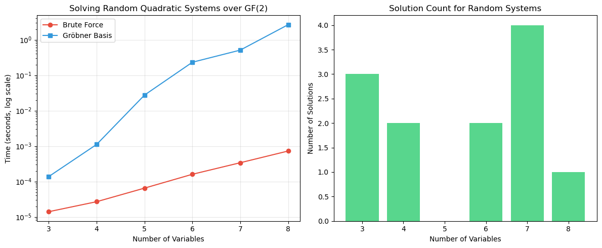
Experiment 1: Solving Random Systems Over GF(2)#
We compare brute-force vs Gröbner basis computation for random quadratic systems of increasing size.
Show code cell source
import numpy as np
import matplotlib.pyplot as plt
import time

def random_quadratic_system(n_vars, n_eqs, rng):
    """Generate a random system of quadratic polynomials over GF(2)."""
    polys = []
    for _ in range(n_eqs):
        terms = []
        # Quadratic terms
        for i in range(n_vars):
            for j in range(i+1, n_vars):
                if rng.random() < 0.3:
                    terms.append(frozenset({i, j}))
        # Linear terms
        for i in range(n_vars):
            if rng.random() < 0.5:
                terms.append(frozenset({i}))
        # Constant
        if rng.random() < 0.5:
            terms.append(frozenset())
        polys.append(GF2Polynomial(terms, n_vars=n_vars))
    return polys

rng = np.random.default_rng(42)
sizes = [3, 4, 5, 6, 7, 8]
bf_times = []
gb_times = []
n_solutions_list = []

for n in sizes:
    system = random_quadratic_system(n, n, rng)

    # Brute force
    t0 = time.time()
    bf_sols = solve_gf2_system(system, n)
    bf_time = time.time() - t0
    bf_times.append(bf_time)

    # Gröbner basis
    t0 = time.time()
    gb = buchberger(system, ordering='grevlex', max_iters=500)
    gb_sols = solve_gf2_system(gb, n)
    gb_time = time.time() - t0
    gb_times.append(gb_time)

    n_solutions_list.append(len(bf_sols))
    print(f'n={n}: {len(bf_sols)} solutions, BF={float(bf_time):.4f}s, GB={float(gb_time):.4f}s')

fig, (ax1, ax2) = plt.subplots(1, 2, figsize=(12, 5))

ax1.semilogy(sizes, bf_times, 'o-', label='Brute Force', color='#e74c3c')
ax1.semilogy(sizes, gb_times, 's-', label='Gröbner Basis', color='#3498db')
ax1.set_xlabel('Number of Variables')
ax1.set_ylabel('Time (seconds, log scale)')
ax1.set_title('Solving Random Quadratic Systems over GF(2)')
ax1.legend()
ax1.grid(True, alpha=0.3)

ax2.bar(sizes, n_solutions_list, color='#2ecc71', alpha=0.8)
ax2.set_xlabel('Number of Variables')
ax2.set_ylabel('Number of Solutions')
ax2.set_title('Solution Count for Random Systems')

plt.tight_layout()
plt.savefig('groebner_timing.png', dpi=150, bbox_inches='tight')
plt.show()
n=3: 3 solutions, BF=0.0000s, GB=0.0001s
n=4: 2 solutions, BF=0.0000s, GB=0.0011s
n=5: 0 solutions, BF=0.0001s, GB=0.0275s
n=6: 2 solutions, BF=0.0002s, GB=0.2323s
n=7: 4 solutions, BF=0.0003s, GB=0.5109s
n=8: 1 solutions, BF=0.0007s, GB=2.6632s
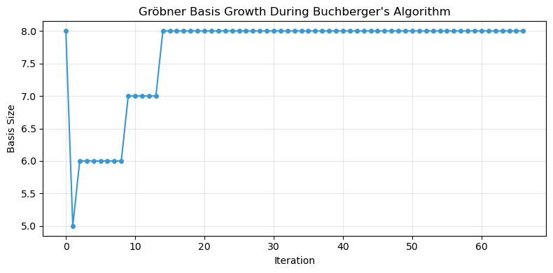
Experiment 2: Visualizing the Reduction Process#
We trace the S-polynomial computations during Buchberger’s algorithm.
Show code cell source
import numpy as np
import matplotlib.pyplot as plt

def buchberger_verbose(F, ordering='grevlex', max_iters=100):
    """Buchberger's algorithm with logging."""
    G = [f for f in F if not f.is_zero()]
    n_vars = G[0].n_vars if G else None

    if n_vars:
        for i in range(n_vars):
            xi = var(i, n_vars)
            G.append(xi * xi + xi)

    pairs = list(combinations(range(len(G)), 2))
    log = {'pairs_checked': 0, 'new_polys': 0, 'basis_sizes': [len(G)]}

    while pairs and log['pairs_checked'] < max_iters:
        i, j = pairs.pop(0)
        if i >= len(G) or j >= len(G):
            continue

        sp = s_polynomial(G[i], G[j], ordering)
        r = reduce_poly(sp, G, ordering)
        log['pairs_checked'] += 1

        if not r.is_zero():
            G.append(r)
            log['new_polys'] += 1
            for k in range(len(G) - 1):
                pairs.append((k, len(G) - 1))

        log['basis_sizes'].append(len([g for g in G if not g.is_zero()]))

    return G, log


# Run on a 4-variable system
n = 4
x = [var(i, n) for i in range(n)]
one = const(1, n)

system = [
    x[0]*x[1] + x[2] + one,
    x[1]*x[2] + x[3],
    x[0]*x[3] + x[1] + x[2],
    x[2]*x[3] + x[0] + one,
]

G, log = buchberger_verbose(system, ordering='grevlex')

print(f'Pairs checked: {log["pairs_checked"]}')
print(f'New polynomials added: {log["new_polys"]}')
print(f'Final basis size: {len([g for g in G if not g.is_zero()])}')

fig, ax = plt.subplots(figsize=(8, 4))
ax.plot(log['basis_sizes'], 'o-', color='#3498db', markersize=4)
ax.set_xlabel('Iteration')
ax.set_ylabel('Basis Size')
ax.set_title('Gröbner Basis Growth During Buchberger\'s Algorithm')
ax.grid(True, alpha=0.3)

plt.tight_layout()
plt.savefig('buchberger_growth.png', dpi=150, bbox_inches='tight')
plt.show()
Pairs checked: 66
New polynomials added: 4
Final basis size: 8
Experiment 3: Application to a Simple Cipher#
We express a 2-bit cipher as a polynomial system and solve for the key.
import numpy as np

# Simple 2-bit cipher: C = S(P XOR K) where S is a nonlinear map
# S-box on 2 bits: S(00)=01, S(01)=11, S(10)=10, S(11)=00
# i.e. S(a,b) = (a XOR b, NOT a) = (a+b, a+1) over GF(2)

# Variables: p0, p1 (plaintext), k0, k1 (key), c0, c1 (ciphertext)
# We know P and C, want to recover K

n = 6  # p0, p1, k0, k1, c0, c1
p0, p1, k0, k1, c0, c1 = [var(i, n) for i in range(n)]
one = const(1, n)

# Internal wires: u0 = p0 + k0, u1 = p1 + k1
# S-box output: c0 = u0 + u1, c1 = u0 + 1
# Substituting: c0 = p0 + k0 + p1 + k1, c1 = p0 + k0 + 1

# Equations from cipher:
eq1 = c0 + p0 + k0 + p1 + k1  # c0 = p0+k0+p1+k1
eq2 = c1 + p0 + k0 + one       # c1 = p0+k0+1

# Known plaintext-ciphertext pair: P=(1,0), C=(0,0)
# Fix known values
eq_p0 = p0 + one   # p0 = 1
eq_p1 = p1          # p1 = 0
eq_c0 = c0          # c0 = 0
eq_c1 = c1          # c1 = 0

system = [eq1, eq2, eq_p0, eq_p1, eq_c0, eq_c1]
print('Cipher equation system:')
for i, eq in enumerate(system):
    print(f'  eq{i}: {eq} = 0')

# Solve
solutions = solve_gf2_system(system, n)
print(f'\nSolutions (p0, p1, k0, k1, c0, c1):')
for sol in solutions:
    print(f'  {sol} -> key = ({sol[2]}, {sol[3]})')

# Verify
print(f'\nRecovered key: k0={solutions[0][2]}, k1={solutions[0][3]}')
print('Verification: P=(1,0) XOR K -> S-box -> C')
u0 = 1 ^ solutions[0][2]
u1 = 0 ^ solutions[0][3]
print(f'  u = ({u0}, {u1}), S(u) = ({u0^u1}, {u0^1}) = ({u0^u1}, {u0^1})')
Cipher equation system:
  eq0: x0 + x1 + x2 + x3 + x4 = 0
  eq1: x0 + x2 + x5 + 1 = 0
  eq2: x0 + 1 = 0
  eq3: x1 = 0
  eq4: x4 = 0
  eq5: x5 = 0

Solutions (p0, p1, k0, k1, c0, c1):
  (1, 0, 0, 1, 0, 0) -> key = (0, 1)

Recovered key: k0=0, k1=1
Verification: P=(1,0) XOR K -> S-box -> C
  u = (1, 1), S(u) = (0, 0) = (0, 0)
Experiment 4: Equation System Size for an SPN#
We count how many equations and variables are needed to express the Heys 3-round SPN as a polynomial system.
Show code cell source
import numpy as np
import matplotlib.pyplot as plt

# The Heys SPN has:
# - 16-bit plaintext, 16-bit ciphertext, 28-bit key
# - 3 rounds, each with 4 S-boxes (4-bit -> 4-bit)
# - Each S-box can be expressed as ~21 quadratic equations in 8 variables (4 in, 4 out)

# Variables per round: 16 (S-box inputs) + 16 (S-box outputs) = 32
# Plus plaintext (16), ciphertext (16), key (28)

# Count for r rounds
def spn_system_size(n_rounds, block_size=16, sbox_size=4, key_size=28):
    n_sboxes_per_round = block_size // sbox_size

    # Variables
    n_internal = 2 * block_size * n_rounds  # S-box inputs and outputs per round
    n_total_vars = block_size + block_size + key_size + n_internal

    # Equations
    # Each S-box: ~21 quadratic equations (for a 4-bit S-box)
    n_sbox_eqs = 21 * n_sboxes_per_round * n_rounds
    # XOR equations (key mixing): 16 linear equations per round
    n_xor_eqs = block_size * n_rounds
    # Permutation: 16 linear equations per round (except last)
    n_perm_eqs = block_size * max(0, n_rounds - 1)
    # Final key addition
    n_final_eqs = block_size

    n_total_eqs = n_sbox_eqs + n_xor_eqs + n_perm_eqs + n_final_eqs

    return n_total_vars, n_total_eqs

rounds_range = range(1, 11)
vars_list = []
eqs_list = []

print(f'{"Rounds":<10} {"Variables":>12} {"Equations":>12} {"Ratio":>8}')
print('=' * 45)

for r in rounds_range:
    v, e = spn_system_size(r)
    vars_list.append(v)
    eqs_list.append(e)
    print(f'{r:<10} {v:>12} {e:>12} {float(e/v):>8.1f}')

fig, ax = plt.subplots(figsize=(8, 5))
ax.plot(list(rounds_range), vars_list, 'o-', label='Variables', color='#3498db')
ax.plot(list(rounds_range), eqs_list, 's-', label='Equations', color='#e74c3c')
ax.set_xlabel('Number of Rounds')
ax.set_ylabel('Count')
ax.set_title('Algebraic System Size for SPN Cipher')
ax.legend()
ax.grid(True, alpha=0.3)

# Mark the 3-round Heys SPN
v3, e3 = spn_system_size(3)
ax.annotate(f'Heys SPN\n({v3} vars, {e3} eqs)', xy=(3, v3),
            xytext=(5, v3+50), arrowprops=dict(arrowstyle='->', color='gray'),
            fontsize=10, ha='center')

plt.tight_layout()
plt.savefig('algebraic_system_size.png', dpi=150, bbox_inches='tight')
plt.show()
Rounds        Variables    Equations    Ratio
=============================================
1                    92          116      1.3
2                   124          232      1.9
3                   156          348      2.2
4                   188          464      2.5
5                   220          580      2.6
6                   252          696      2.8
7                   284          812      2.9
8                   316          928      2.9
9                   348         1044      3.0
10                  380         1160      3.1
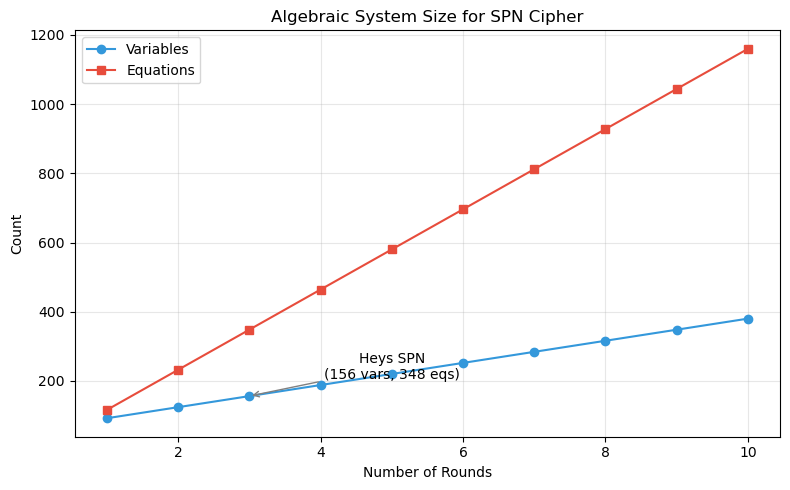
Observation
For the 3-round Heys SPN, the algebraic system has approximately 156 variables and 348 equations. For AES-128 (10 rounds, 128-bit blocks), the system would have thousands of variables and equations — still within reach of theory but far beyond current Gröbner basis solvers for the general case.
Danger
While the number of equations grows linearly with rounds, the complexity of solving the system grows exponentially (or worse) with the number of variables. This is why algebraic attacks have not broken AES in practice, despite the polynomial system being expressible.
34.5 Exercises#
Exercise 34.1 (Warm-up) Compute \(S(f, g)\) by hand for \(f = x_0 x_1 + x_2\) and \(g = x_0 x_2 + 1\) over \(\mathrm{GF}(2)\) with grevlex ordering.
Hint
\(\mathrm{LT}(f) = x_0 x_1\), \(\mathrm{LT}(g) = x_0 x_2\). \(\mathrm{lcm} = x_0 x_1 x_2\). Quotients: \(x_2\) and \(x_1\). \(S(f,g) = x_2 f + x_1 g\).
Exercise 34.2 (Applied) Implement a reduced Gröbner basis by adding an inter-reduction step that removes redundant elements and makes all leading coefficients 1 (automatic over GF(2)).
Hint
After Buchberger terminates, for each \(g_i \in G\), check if \(\mathrm{LT}(g_i)\) is divisible by \(\mathrm{LT}(g_j)\) for any \(j \neq i\). If so, remove \(g_i\). Then reduce each remaining element modulo the others.
Exercise 34.3 (Analysis) Express the Heys 4-bit S-box as a system of quadratic equations over \(\mathrm{GF}(2)\). How many equations do you need? Verify that they have exactly 16 solutions (one per input).
Hint
Introduce 4 input variables and 4 output variables. For each input-output pair \((x, S(x))\), the point must satisfy all equations. The equations come from the algebraic normal form of each output bit.
Exercise 34.4 (Theory) Prove that over \(\mathrm{GF}(2)\), any Boolean function on \(n\) variables can be uniquely expressed in algebraic normal form (ANF).
Hint
There are \(2^{2^n}\) Boolean functions on \(n\) variables and \(2^{2^n}\) possible ANF polynomials (each of \(2^n\) monomials is either present or absent). Show that the Möbius transform gives a bijection between truth tables and ANF.
Exercise 34.5 (Challenge) Implement the F4 or F5 algorithm, which improves on Buchberger by processing multiple S-polynomials simultaneously using linear algebra. Compare its performance to your Buchberger implementation.
Hint
F4 (Faugère 1999) constructs a matrix where rows represent polynomials and columns represent monomials, then uses Gaussian elimination to reduce many S-polynomials at once. This is much more efficient for larger systems.
34.6 Summary#
Concept |
Key Point |
|---|---|
Gröbner basis |
Generalization of Gaussian elimination to nonlinear systems |
Buchberger’s algorithm |
Computes GB via S-polynomial reduction |
\(\mathrm{GF}(2)\) specialization |
Field equations \(x_i^2 = x_i\) keep degree bounded |
Monomial orderings |
Lex gives triangular form; grevlex is faster to compute |
Cipher modeling |
Any cipher = system of polynomial equations over \(\mathrm{GF}(2)\) |
Scalability |
System size grows linearly with rounds; solving grows exponentially |
Tip
Gröbner bases provide the theoretical foundation for algebraic cryptanalysis. In Chapter 35, we will use them to model S-boxes algebraically, and in Chapter 36, we will attempt to attack the Heys SPN using algebraic techniques.
References#
Buchberger, B. (1965). An Algorithm for Finding the Basis Elements of the Residue Class Ring of a Zero-Dimensional Polynomial Ideal. PhD thesis, University of Innsbruck.
Courtois, N. T. and Pieprzyk, J. (2002). Cryptanalysis of Block Ciphers with Overdefined Systems of Equations. ASIACRYPT 2002, LNCS 2501, 267–287.
Faugère, J.-C. (1999). A New Efficient Algorithm for Computing Gröbner Bases (F4). Journal of Pure and Applied Algebra, 139, 61–88.
Bard, G. V. (2009). Algebraic Cryptanalysis. Springer.
Cox, D., Little, J., and O’Shea, D. (2015). Ideals, Varieties, and Algorithms. 4th ed., Springer.