Chapter 44: NIST Post-Quantum Cryptography Standards

Chapter 44: NIST Post-Quantum Cryptography Standards#

The transition to post-quantum cryptography represents one of the most significant coordinated efforts in the history of cryptographic standardization. In 2016, the U.S. National Institute of Standards and Technology (NIST) launched an open competition to develop cryptographic algorithms resistant to attacks by both classical and quantum computers. After eight years of rigorous evaluation spanning three rounds, NIST published its first post-quantum cryptographic standards in 2024: ML-KEM (FIPS 203), ML-DSA (FIPS 204), and SLH-DSA (FIPS 205).

This chapter surveys the competition timeline, examines each finalized standard and its parameters, compares key sizes, ciphertext sizes, and performance characteristics, and provides a migration roadmap for practitioners.

44.1 History of the NIST PQC Competition#

The NIST Post-Quantum Cryptography Standardization Process was motivated by the recognition that large-scale quantum computers, once realized, would break the public-key cryptographic algorithms (RSA, ECC, DH) currently securing the internet.

Shor’s Algorithm Threat

Shor’s algorithm (1994) can factor integers and compute discrete logarithms in polynomial time on a quantum computer. This renders RSA, DSA, ECDSA, and ECDH insecure against a sufficiently powerful quantum adversary.

Timeline#

Year	Milestone
2016	NIST announces the PQC Standardization Process; call for proposals
2017	69 complete and proper submissions received (82 total)
2019	Round 2: 26 algorithms advance (17 PKE/KEM + 9 signatures)
2020	Round 3: 7 finalists + 8 alternate candidates
2022	NIST announces first selections: CRYSTALS-Kyber, CRYSTALS-Dilithium, FALCON, SPHINCS+
2023	Draft standards published for public comment
2024	Final standards published: FIPS 203 (ML-KEM), FIPS 204 (ML-DSA), FIPS 205 (SLH-DSA)
2025	HQC selected for standardization as the 4th-round KEM (code-based alternative to ML-KEM)
TBD	FALCON/FN-DSA (draft FIPS 206) remains in development; not yet a final FIPS standard

../_images/953788d9a324ff2484196215945bed97c65f698550549ae4a2d5fdbd083323ec.png

Figure 44.1. The NIST PQC standardization process spanned eight years from the initial call for proposals in 2016 to the publication of three final standards in August 2024. The process involved progressively narrowing the candidate pool through three evaluation rounds.

Selection Criteria

NIST evaluated candidates on three primary axes: (1) security – provable reductions, concrete security estimates, and resistance to known attacks; (2) performance – speed of key generation, encapsulation/signing, and decapsulation/verification; (3) characteristics – key and ciphertext sizes, bandwidth requirements, and implementation complexity.

44.2 The Finalized Standards#

NIST published three standards in August 2024, each based on a finalist from the competition:

FIPS 203: ML-KEM (Module-Lattice-Based Key-Encapsulation Mechanism)#

Based on CRYSTALS-Kyber, ML-KEM is a lattice-based key encapsulation mechanism built on the Module Learning With Errors (MLWE) problem. It provides IND-CCA2 security through a Fujisaki-Okamoto transform.

Three parameter sets: ML-KEM-512, ML-KEM-768, ML-KEM-1024
Underlying hard problem: Module-LWE over polynomial rings
Primary use case: Key establishment (replacing ECDH/RSA key exchange)

FIPS 204: ML-DSA (Module-Lattice-Based Digital Signature Algorithm)#

Based on CRYSTALS-Dilithium, ML-DSA is a lattice-based digital signature scheme built on the Module-LWE and Module-SIS (Short Integer Solution) problems.

Three parameter sets: ML-DSA-44, ML-DSA-65, ML-DSA-87
Underlying hard problem: Module-LWE + Module-SIS
Primary use case: Digital signatures (replacing ECDSA/RSA signatures)

FIPS 205: SLH-DSA (Stateless Hash-Based Digital Signature Algorithm)#

Based on SPHINCS+, SLH-DSA is a hash-based digital signature scheme whose security relies solely on the properties of the underlying hash function. It serves as a conservative backup to lattice-based signatures.

Twelve parameter sets: Combinations of security levels (128/192/256), hash functions (SHA-256, SHAKE), and optimization targets (small signatures vs. fast signing)
Underlying hard problem: Hash function security (second preimage resistance)
Primary use case: Conservative signature scheme with minimal assumptions

Why Multiple Standards?

NIST intentionally standardized algorithms based on different mathematical problems. If a breakthrough attack is found against lattice-based schemes (ML-KEM, ML-DSA), the hash-based SLH-DSA provides a fallback with security assumptions rooted only in hash function properties, which are much better understood.

import numpy as np
import matplotlib.pyplot as plt

# --- NIST Security Levels and Corresponding Parameter Sets ---
# NIST defines 5 security levels based on brute-force equivalence
security_levels = {
    'Level 1': {'bits': 128, 'equivalent': 'AES-128 key search',
                'algorithms': ['ML-KEM-512', 'SLH-DSA-128s/f']},
    'Level 2': {'bits': 128, 'equivalent': 'SHA-256 collision',
                'algorithms': ['ML-DSA-44']},
    'Level 3': {'bits': 192, 'equivalent': 'AES-192 key search',
                'algorithms': ['ML-KEM-768', 'ML-DSA-65', 'SLH-DSA-192s/f']},
    'Level 4': {'bits': 192, 'equivalent': 'SHA-384 collision',
                'algorithms': []},
    'Level 5': {'bits': 256, 'equivalent': 'AES-256 key search',
                'algorithms': ['ML-KEM-1024', 'ML-DSA-87', 'SLH-DSA-256s/f']},
}

print("NIST Post-Quantum Security Levels")
print("=" * 72)
print(f"{'Level':<10} {'Classical Bits':<16} {'Equivalence':<25} {'Algorithms'}")
print("-" * 72)
for level, info in security_levels.items():
    algs = ', '.join(info['algorithms']) if info['algorithms'] else '(none standardized)'
    print(f"{level:<10} {info['bits']:<16} {info['equivalent']:<25} {algs}")
print("\nNote: Levels are defined by the cost of the best quantum attack.")
print("Level 1 >= 2^128 quantum gates (matching AES-128 exhaustive search).")

NIST Post-Quantum Security Levels
========================================================================
Level      Classical Bits   Equivalence               Algorithms
------------------------------------------------------------------------
Level 1    128              AES-128 key search        ML-KEM-512, SLH-DSA-128s/f
Level 2    128              SHA-256 collision         ML-DSA-44
Level 3    192              AES-192 key search        ML-KEM-768, ML-DSA-65, SLH-DSA-192s/f
Level 4    192              SHA-384 collision         (none standardized)
Level 5    256              AES-256 key search        ML-KEM-1024, ML-DSA-87, SLH-DSA-256s/f

Note: Levels are defined by the cost of the best quantum attack.
Level 1 >= 2^128 quantum gates (matching AES-128 exhaustive search).

44.3 ML-KEM Parameter Details (FIPS 203)#

ML-KEM operates over the polynomial ring \(R_q = \mathbb{Z}_q[X]/(X^n + 1)\) with \(n = 256\) and \(q = 3329\). The module rank \(k\) determines the security level:

Parameter	ML-KEM-512	ML-KEM-768	ML-KEM-1024
Module rank \(k\)	2	3	4
NIST security level	1	3	5
Public key (bytes)	800	1,184	1,568
Secret key (bytes)	1,632	2,400	3,168
Ciphertext (bytes)	768	1,088	1,568
Shared secret (bytes)	32	32	32
Encaps failure prob.	\(2^{-139}\)	\(2^{-164}\)	\(2^{-174}\)

../_images/961d46884308d82c7b07b505d1fc41053445a32c76de4bf9167df7693f4396a0.png

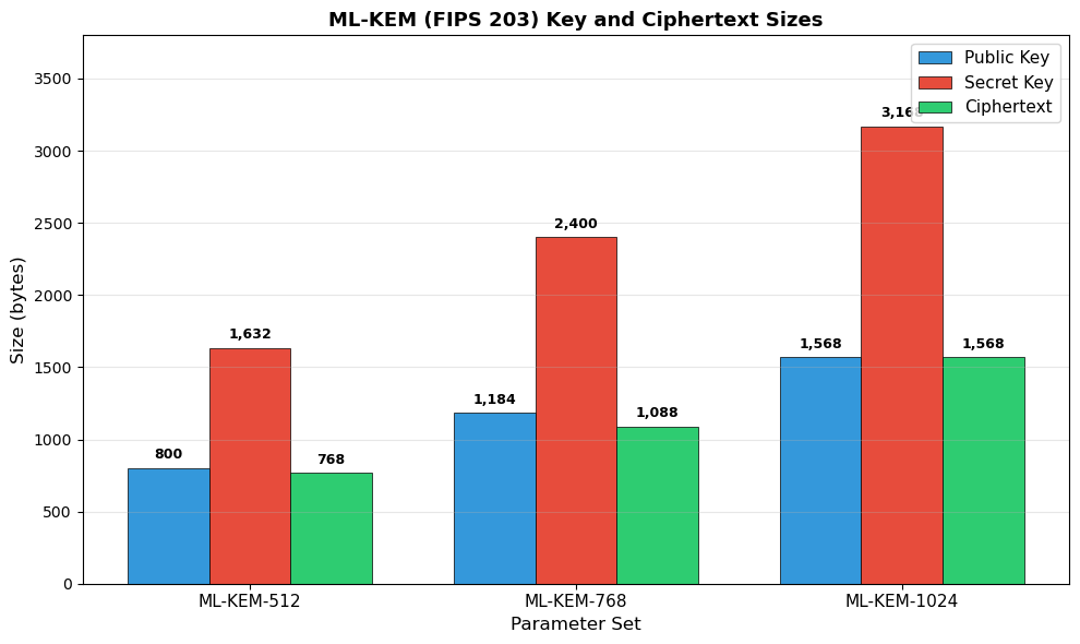
Figure 44.2. ML-KEM key and ciphertext sizes across parameter sets. Even at the highest security level (ML-KEM-1024), the public key is only 1,568 bytes, making ML-KEM very practical for most applications. The shared secret is always 32 bytes regardless of parameter set.

Comparison with RSA

An RSA-2048 public key is 256 bytes, but an RSA-3072 key (roughly equivalent to AES-128 security) is 384 bytes. ML-KEM-512 at 800 bytes is roughly 2–3x larger, but the ciphertext is comparable, and the computational cost is dramatically lower than RSA.

44.4 ML-DSA Parameter Details (FIPS 204)#

ML-DSA (based on Dilithium) also operates over polynomial rings with \(q = 8\,380\,417\) and \(n = 256\). The parameters \((k, \ell)\) define the module dimensions:

Parameter	ML-DSA-44	ML-DSA-65	ML-DSA-87
\((k, \ell)\)	\((4, 4)\)	\((6, 5)\)	\((8, 7)\)
NIST security level	2	3	5
Public key (bytes)	1,312	1,952	2,592
Secret key (bytes)	2,560	4,032	4,896
Signature (bytes)	2,420	3,309	4,627

../_images/8982df9abc356712778e2287cf9e5661eb886b46fea055206c7fc06506a447d4.png

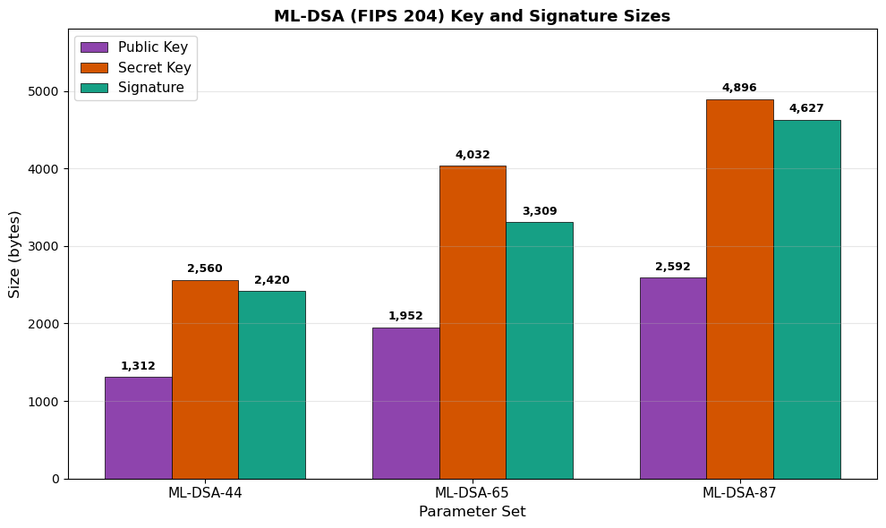
Figure 44.3. ML-DSA key and signature sizes.

Signatures range from about 2.4 KB to 4.6 KB, which is significantly larger than ECDSA signatures (~64 bytes) but far more compact than the hash-based alternative SLH-DSA.

44.5 SLH-DSA Parameter Details (FIPS 205)#

SLH-DSA (based on SPHINCS+) provides twelve parameter sets, organized along three axes:

Security level: 128, 192, or 256 bits
Hash function: SHA-256 or SHAKE-256 (each security level has both SHA2 and SHAKE variants)
Optimization: s (small signatures) or f (fast signing)

Parameter Set	Security Level	Public Key	Secret Key	Signature
SLH-DSA-SHA2-128s	1	32 B	64 B	7,856 B
SLH-DSA-SHA2-128f	1	32 B	64 B	17,088 B
SLH-DSA-SHA2-192s	3	48 B	96 B	16,224 B
SLH-DSA-SHA2-192f	3	48 B	96 B	35,664 B
SLH-DSA-SHA2-256s	5	64 B	128 B	29,792 B
SLH-DSA-SHA2-256f	5	64 B	128 B	49,856 B
SLH-DSA-SHAKE-128s	1	32 B	64 B	7,856 B
SLH-DSA-SHAKE-128f	1	32 B	64 B	17,088 B
SLH-DSA-SHAKE-192s	3	48 B	96 B	16,224 B
SLH-DSA-SHAKE-192f	3	48 B	96 B	35,664 B
SLH-DSA-SHAKE-256s	5	64 B	128 B	29,792 B
SLH-DSA-SHAKE-256f	5	64 B	128 B	49,856 B

SLH-DSA Trade-off

SLH-DSA keys are tiny (32–64 bytes for public keys), but signatures are very large (up to ~49 KB). The s (small) variants produce smaller signatures at the cost of slower signing; the f (fast) variants sign quickly but produce much larger signatures. This trade-off is fundamental to hash-based signature schemes.

../_images/c2179e3a6b246502cfc8cf53782bf045f1499819ef6cdad881ec7313eeb5a460.png

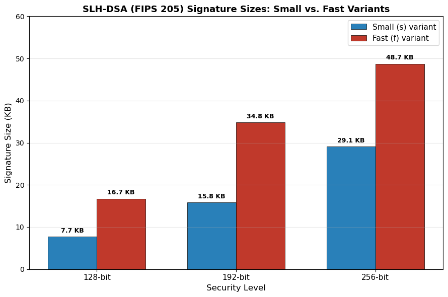
Figure 44.4. SLH-DSA signature sizes for small and fast variants.

The fast variants trade signature compactness for significantly faster signing speeds. At the 256-bit security level, signatures approach 50 KB, which is three orders of magnitude larger than ECDSA.

44.6 Additional Candidates: Classic McEliece and HQC#

Beyond the three finalized standards, NIST has continued evaluating additional KEM candidates:

Classic McEliece#

Basis: Binary Goppa codes (code-based cryptography)
History: Based on McEliece’s 1978 cryptosystem, the oldest unbroken public-key scheme
Strength: Very large public keys but extremely small ciphertexts; decades of cryptanalytic scrutiny
Weakness: Public keys range from ~261 KB to ~1.3 MB

HQC (Hamming Quasi-Cyclic)#

Basis: Quasi-cyclic codes over structured error-correcting codes
Selected by NIST on March 11, 2025 for standardization as a code-based KEM alternative to ML-KEM
Advantage: Provides diversity from lattice-based ML-KEM

Algorithmic Diversity

NIST’s strategy of standardizing algorithms from different mathematical families (lattices, hashes, codes) ensures that a cryptanalytic breakthrough against one family does not compromise all post-quantum security.

Show code cell source Hide code cell source

import numpy as np
import matplotlib.pyplot as plt

# --- Cross-Algorithm KEM Comparison ---
algorithms = [
    'RSA-2048\n(classical)',
    'ECDH P-256\n(classical)',
    'ML-KEM-512',
    'ML-KEM-768',
    'ML-KEM-1024',
    'Classic McEliece\n348864',
    'Classic McEliece\n6960119',
    'HQC-128',
    'HQC-256',
]

# Public key sizes in bytes
pk_sizes = np.array([256, 64, 800, 1184, 1568, 261120, 1047319, 2249, 7989])
# Ciphertext sizes in bytes
ct_sizes = np.array([256, 64, 768, 1088, 1568, 128, 226, 4497, 15973])

fig, (ax1, ax2) = plt.subplots(1, 2, figsize=(16, 7))

# Public key sizes (log scale)
colors_pk = ['#95a5a6', '#95a5a6', '#3498db', '#2980b9', '#1a5276',
             '#e74c3c', '#c0392b', '#27ae60', '#1e8449']
bars1 = ax1.barh(range(len(algorithms)), pk_sizes, color=colors_pk,
                 edgecolor='black', linewidth=0.5)
ax1.set_xscale('log')
ax1.set_yticks(range(len(algorithms)))
ax1.set_yticklabels(algorithms, fontsize=9)
ax1.set_xlabel('Public Key Size (bytes, log scale)', fontsize=11)
ax1.set_title('Public Key Sizes', fontsize=12, fontweight='bold')
ax1.invert_yaxis()
ax1.grid(axis='x', alpha=0.3)

# Annotate with actual values
for i, (v, bar) in enumerate(zip(pk_sizes, bars1)):
    if v >= 1024:
        label = f'{float(v/1024):.0f} KB' if v < 1048576 else f'{float(v/1048576):.1f} MB'
    else:
        label = f'{v} B'
    ax1.text(v * 1.3, i, label, va='center', fontsize=8, fontweight='bold')

# Ciphertext sizes (log scale)
bars2 = ax2.barh(range(len(algorithms)), ct_sizes, color=colors_pk,
                 edgecolor='black', linewidth=0.5)
ax2.set_xscale('log')
ax2.set_yticks(range(len(algorithms)))
ax2.set_yticklabels(algorithms, fontsize=9)
ax2.set_xlabel('Ciphertext Size (bytes, log scale)', fontsize=11)
ax2.set_title('Ciphertext / Encapsulated Key Sizes', fontsize=12, fontweight='bold')
ax2.invert_yaxis()
ax2.grid(axis='x', alpha=0.3)

for i, (v, bar) in enumerate(zip(ct_sizes, bars2)):
    if v >= 1024:
        label = f'{float(v/1024):.1f} KB'
    else:
        label = f'{v} B'
    ax2.text(v * 1.3, i, label, va='center', fontsize=8, fontweight='bold')

plt.tight_layout()
plt.savefig('fig_ch44_kem_comparison.png', dpi=150, bbox_inches='tight')
plt.show()

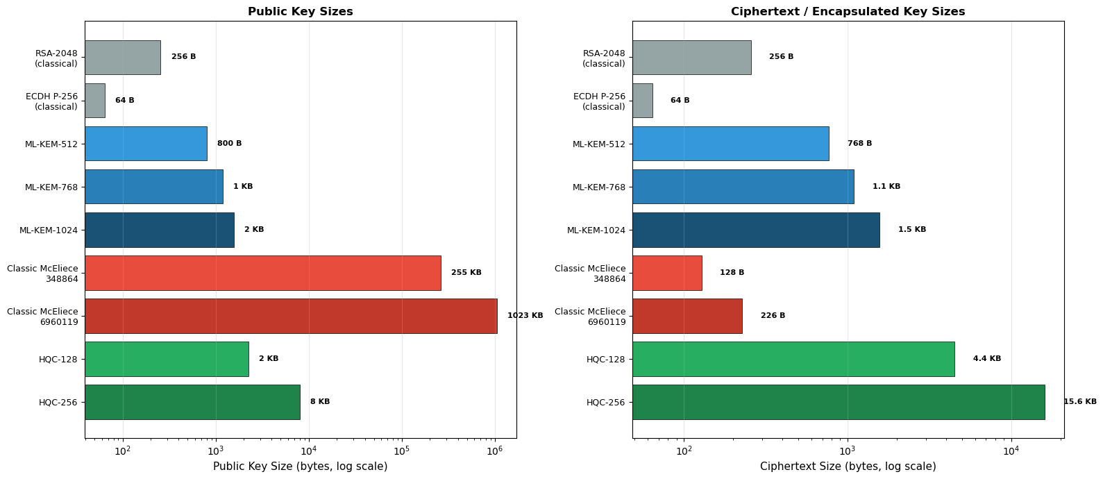
../_images/0f67673859e270f1a40ddcf7ae8a4f29f4d8868ed8e030554f469c564f6ce4c6.png

Figure 44.5. Cross-algorithm comparison of KEM public key and ciphertext sizes on a logarithmic scale.

Classic McEliece has by far the largest public keys (261 KB to 1 MB+) but the smallest ciphertexts. ML-KEM offers the best balance for most applications. HQC provides a code-based alternative with moderate sizes.

44.7 Signature Scheme Cross-Comparison#

Comparing the standardized PQ signature schemes and FALCON alongside classical algorithms reveals the trade-offs inherent in post-quantum cryptography.

Show code cell source Hide code cell source

import numpy as np
import matplotlib.pyplot as plt

# --- Signature Scheme Comparison: PK + Signature Combined Bandwidth ---
schemes = [
    'RSA-2048', 'ECDSA P-256', 'Ed25519',
    'ML-DSA-44', 'ML-DSA-65', 'ML-DSA-87',
    'SLH-DSA-128s', 'SLH-DSA-128f',
    'SLH-DSA-256s', 'SLH-DSA-256f',
    'FALCON-512', 'FALCON-1024'
]

pk_bytes = np.array([256, 64, 32,
                     1312, 1952, 2592,
                     32, 32, 64, 64,
                     897, 1793])

sig_bytes = np.array([256, 64, 64,
                      2420, 3309, 4627,
                      7856, 17088, 29792, 49856,
                      666, 1280])

# Color by family
colors_sig = ['#bdc3c7'] * 3 + ['#3498db'] * 3 + ['#e74c3c'] * 4 + ['#f39c12'] * 2

fig, ax = plt.subplots(figsize=(12, 7))

y_pos = np.arange(len(schemes))
bars_pk = ax.barh(y_pos, pk_bytes, height=0.4, label='Public Key',
                  color=[c for c in colors_sig], alpha=0.6,
                  edgecolor='black', linewidth=0.5)
bars_sig = ax.barh(y_pos, sig_bytes, height=0.4, left=pk_bytes,
                   label='Signature', color=[c for c in colors_sig], alpha=1.0,
                   edgecolor='black', linewidth=0.5)

ax.set_xscale('log')
ax.set_yticks(y_pos)
ax.set_yticklabels(schemes, fontsize=9)
ax.set_xlabel('Combined Size: Public Key + Signature (bytes, log scale)', fontsize=11)
ax.set_title('Digital Signature Schemes: Total Transmission Cost',
             fontsize=13, fontweight='bold')
ax.invert_yaxis()
ax.grid(axis='x', alpha=0.3)

# Add total annotations
for i in range(len(schemes)):
    total = pk_bytes[i] + sig_bytes[i]
    if total >= 1024:
        label = f'{float(total/1024):.1f} KB'
    else:
        label = f'{total} B'
    ax.text(total * 1.2, i, label, va='center', fontsize=8, fontweight='bold')

# Custom legend
from matplotlib.patches import Patch
legend_elements = [
    Patch(facecolor='#bdc3c7', edgecolor='black', label='Classical'),
    Patch(facecolor='#3498db', edgecolor='black', label='ML-DSA (lattice)'),
    Patch(facecolor='#e74c3c', edgecolor='black', label='SLH-DSA (hash)'),
    Patch(facecolor='#f39c12', edgecolor='black', label='FALCON (lattice)'),
]
ax.legend(handles=legend_elements, loc='lower right', fontsize=10)

plt.tight_layout()
plt.savefig('fig_ch44_sig_comparison.png', dpi=150, bbox_inches='tight')
plt.show()

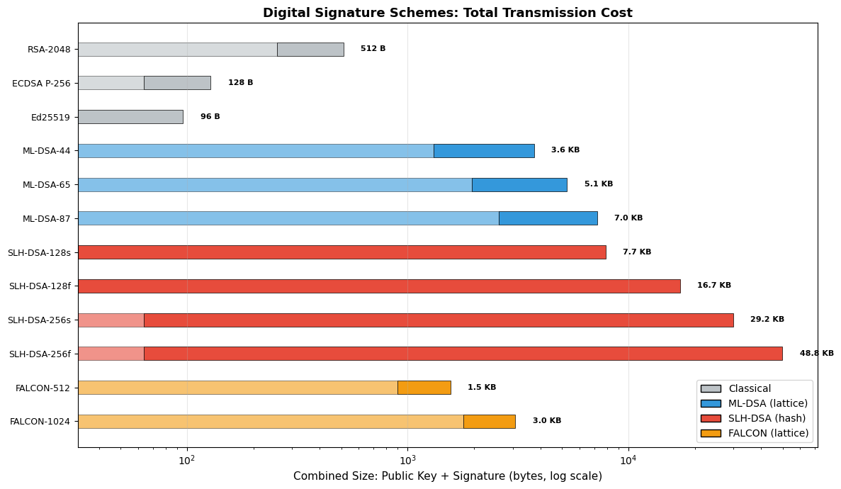
../_images/6e71fb28ff6d58cf419f807bfbdb15ea90153d0190b0e2c28eb787015905cb86.png

Figure 44.6. Total transmission cost (public key + signature) for classical and post-quantum signature schemes. FALCON (selected but not yet standardized) achieves the most compact PQ signatures. ML-DSA offers a good balance. SLH-DSA signatures are large but provide the strongest security assumptions.

FALCON Status

FALCON was selected by NIST alongside Dilithium and SPHINCS+ in 2022 but has not yet been published as a final FIPS standard. A draft standard (FIPS 206, FN-DSA) remains in development as of early 2025 and is not yet finalized. FALCON offers the most compact lattice-based signatures but is harder to implement securely due to its reliance on floating-point arithmetic in sampling.

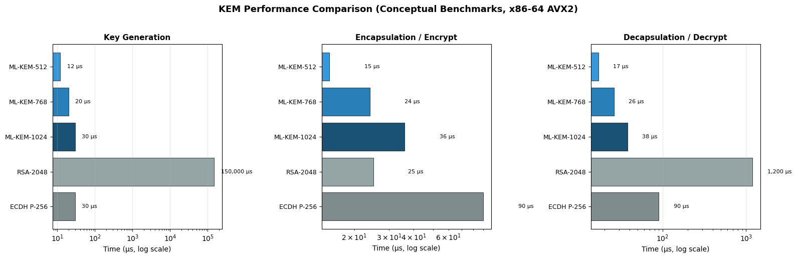
44.8 Conceptual Performance Benchmarks#

The following performance data is based on published benchmarks from the NIST submissions and independent evaluations on modern x86-64 hardware (with AVX2 acceleration).

Benchmark Caveat

Actual performance varies significantly with hardware, compiler optimizations, and implementation choices. The values below are representative of optimized C/AVX2 implementations and are intended for relative comparison only.

../_images/67bdb8461b3d67d888c238e66039fcb9af0419dcb5b4fffe60514ce1f27fe0f7.png

Show code cell source Hide code cell source

import numpy as np
import matplotlib.pyplot as plt

# --- Signature Performance Benchmarks (conceptual, microseconds) ---
sig_data = {
    'ML-DSA-44':     {'keygen': 30,   'sign': 100,   'verify': 30},
    'ML-DSA-65':     {'keygen': 50,   'sign': 170,   'verify': 50},
    'ML-DSA-87':     {'keygen': 75,   'sign': 230,   'verify': 80},
    'SLH-DSA-128s':  {'keygen': 5,    'sign': 260000, 'verify': 7000},
    'SLH-DSA-128f':  {'keygen': 5,    'sign': 8000,  'verify': 500},
    'ECDSA P-256':   {'keygen': 30,   'sign': 40,    'verify': 90},
    'RSA-2048':      {'keygen': 150000, 'sign': 1200, 'verify': 25},
}

algo_names_sig = list(sig_data.keys())
colors_sig_perf = ['#3498db', '#2980b9', '#1a5276',
                   '#e74c3c', '#c0392b',
                   '#95a5a6', '#7f8c8d']

fig, axes = plt.subplots(1, 3, figsize=(16, 6))
operations_sig = ['keygen', 'sign', 'verify']
op_labels_sig = ['Key Generation', 'Signing', 'Verification']

for idx, (op, op_label) in enumerate(zip(operations_sig, op_labels_sig)):
    values = [sig_data[alg][op] for alg in algo_names_sig]
    ax = axes[idx]
    bars = ax.barh(range(len(algo_names_sig)), values, color=colors_sig_perf,
                   edgecolor='black', linewidth=0.5)
    ax.set_xscale('log')
    ax.set_yticks(range(len(algo_names_sig)))
    ax.set_yticklabels(algo_names_sig, fontsize=9)
    ax.set_xlabel('Time (\u00b5s, log scale)', fontsize=10)
    ax.set_title(op_label, fontsize=11, fontweight='bold')
    ax.invert_yaxis()
    ax.grid(axis='x', alpha=0.3)
    for i, v in enumerate(values):
        if v >= 1000:
            label = f'{float(v/1000):.0f} ms'
        else:
            label = f'{v} \u00b5s'
        ax.text(v * 1.5, i, label, va='center', fontsize=8)

plt.suptitle('Signature Performance Comparison (Conceptual Benchmarks, x86-64 AVX2)',
             fontsize=13, fontweight='bold', y=1.02)
plt.tight_layout()
plt.savefig('fig_ch44_sig_performance.png', dpi=150, bbox_inches='tight')
plt.show()

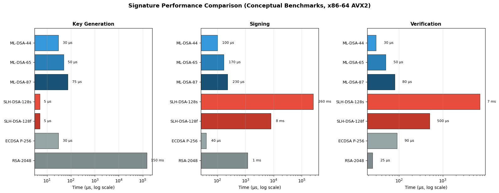
../_images/760ec39c631ddee7c02e2c752c488fc2fcf103000870282cd96d023482c9ae6f.png

Figures 44.7–44.8. Performance benchmarks for KEM and signature schemes. ML-KEM is remarkably fast, outperforming both RSA and ECDH in encapsulation and decapsulation. ML-DSA signing and verification are competitive with ECDSA. SLH-DSA-128s signing is extremely slow (~260 ms) compared to ML-DSA-44 (~100 microseconds), a factor of 2,600x.

ML-KEM Speed Advantage

ML-KEM operations are dominated by polynomial multiplications in \(\mathbb{Z}_q[X]/(X^{256}+1)\) using the Number Theoretic Transform (NTT), which takes only hundreds of cycles on modern hardware. This makes ML-KEM one of the fastest KEM schemes ever standardized.

44.9 Security Level Analysis and Quantum Threat Timeline#

A central question for migration planning is: when will a cryptographically relevant quantum computer (CRQC) exist? Estimates vary widely, but most experts place the timeline between 2030 and 2045+ for a machine capable of breaking RSA-2048.

../_images/c987213a5bc8a922673b1fdb24b94c99f4b8196dc47470e31649f2c7e87f96c7.png

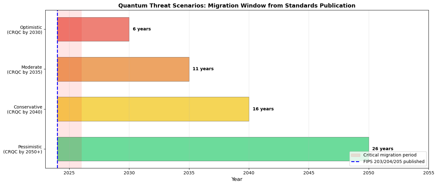
Figure 44.9. Migration windows under different quantum threat scenarios. Even in the most conservative scenario, organizations have limited time to complete migration. The “harvest now, decrypt later” (HNDL) threat means that encrypted data captured today can be stored and decrypted once quantum computers become available, making migration urgent for long-lived secrets.

Harvest Now, Decrypt Later (HNDL)

Adversaries can intercept and store encrypted communications today, then decrypt them once a quantum computer is available. This means that data requiring confidentiality for more than 10–15 years is already at risk and should be protected with post-quantum key exchange immediately.

44.10 Migration Roadmap#

NIST, NSA (via CNSA 2.0), and other agencies have published migration guidance. The key principles are:

Inventory: Catalog all cryptographic assets and dependencies
Prioritize: Protect long-lived secrets first (HNDL threat)
Hybrid mode: Use hybrid classical+PQ schemes during transition
Test: Validate interoperability and performance
Deploy: Roll out PQ algorithms with monitoring

../_images/7855278922dad215885109c3ffb2adc3d11d58ea8fef8c693272909c79706208.png

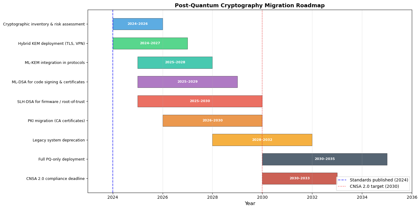
Figure 44.10. A representative migration roadmap for organizations transitioning to post-quantum cryptography.

Key exchange (ML-KEM) should be prioritized due to the HNDL threat.

Signature migration can follow, with SLH-DSA reserved for high-assurance applications like firmware signing.

44.11 Bandwidth Impact Analysis#

One of the most practical concerns for PQC migration is the increase in bandwidth. Let us quantify the impact on a TLS 1.3 handshake.

Show code cell source Hide code cell source

import numpy as np
import matplotlib.pyplot as plt

# --- TLS Handshake Size Impact ---
# Simplified model: handshake involves key exchange + server signature + certificate chain

configs = {
    'Classical\n(ECDHE + ECDSA)': {
        'KEM PK': 64, 'KEM CT': 64, 'Sig PK': 64, 'Signature': 64,
    },
    'Hybrid\n(ECDHE+ML-KEM-768\n+ ECDSA+ML-DSA-65)': {
        'KEM PK': 64 + 1184, 'KEM CT': 64 + 1088,
        'Sig PK': 64 + 1952, 'Signature': 64 + 3309,
    },
    'PQ-Only\n(ML-KEM-768\n+ ML-DSA-65)': {
        'KEM PK': 1184, 'KEM CT': 1088,
        'Sig PK': 1952, 'Signature': 3309,
    },
    'PQ Conservative\n(ML-KEM-1024\n+ SLH-DSA-128s)': {
        'KEM PK': 1568, 'KEM CT': 1568,
        'Sig PK': 32, 'Signature': 7856,
    },
}

config_names = list(configs.keys())
components = ['KEM PK', 'KEM CT', 'Sig PK', 'Signature']
comp_colors = ['#3498db', '#2ecc71', '#e74c3c', '#f39c12']

fig, ax = plt.subplots(figsize=(12, 6))

x = np.arange(len(config_names))
bottoms = np.zeros(len(config_names))

for comp, color in zip(components, comp_colors):
    values = np.array([configs[c][comp] for c in config_names])
    ax.bar(x, values, bottom=bottoms, label=comp, color=color,
           edgecolor='black', linewidth=0.5, width=0.6)
    # Label each segment
    for i, (v, b) in enumerate(zip(values, bottoms)):
        if v > 300:
            ax.text(i, b + v/2, f'{float(v/1024):.1f}K', ha='center', va='center',
                    fontsize=8, fontweight='bold', color='white')
    bottoms += values

# Total labels on top
for i, total in enumerate(bottoms):
    ax.text(i, total + 100, f'Total: {float(total/1024):.1f} KB',
            ha='center', va='bottom', fontsize=9, fontweight='bold')

ax.set_xticks(x)
ax.set_xticklabels(config_names, fontsize=9)
ax.set_ylabel('Handshake Crypto Payload (bytes)', fontsize=11)
ax.set_title('TLS 1.3 Handshake: Cryptographic Payload Size by Configuration',
             fontsize=13, fontweight='bold')
ax.legend(fontsize=10)
ax.grid(axis='y', alpha=0.3)
ax.set_ylim(0, max(bottoms) * 1.15)

plt.tight_layout()
plt.savefig('fig_ch44_tls_bandwidth.png', dpi=150, bbox_inches='tight')
plt.show()

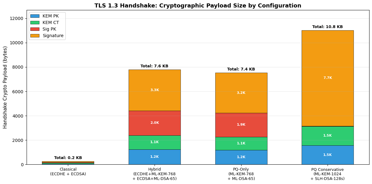
../_images/82e54a555c573cddea3be0d8bbb0ba6668041fae21bca8f6db59e314bf896227.png

Figure 44.11. Cryptographic payload sizes in a TLS 1.3 handshake under different configurations.

The hybrid configuration approximately doubles the payload compared to PQ-only, since both classical and PQ artifacts are transmitted.

Even with PQ-only ML-KEM + ML-DSA, the total handshake overhead is about 7.5 KB, which is manageable for most networks but may matter for constrained IoT devices.

44.12 Lattice Parameter Geometry#

Both ML-KEM and ML-DSA are built on lattice problems. Let us visualize the core idea: finding short vectors in a lattice is computationally hard.

Show code cell source Hide code cell source

import numpy as np
import matplotlib.pyplot as plt

# --- 2D Lattice Visualization with LWE Error ---
np.random.seed(44)

# Define a 2D lattice basis
B = np.array([[1.0, 0.3],
              [0.2, 1.1]])

# Generate lattice points
coords = np.arange(-5, 6)
lattice_points = []
for i in coords:
    for j in coords:
        point = i * B[0] + j * B[1]
        lattice_points.append(point)
lattice_points = np.array(lattice_points)

fig, (ax1, ax2) = plt.subplots(1, 2, figsize=(14, 6))

# Left: Clean lattice with shortest vector highlighted
ax1.scatter(lattice_points[:, 0], lattice_points[:, 1], c='#2c3e50', s=20, zorder=3)
ax1.scatter([0], [0], c='red', s=100, zorder=4, marker='*', label='Origin')

# Highlight shortest nonzero vectors
norms = np.linalg.norm(lattice_points, axis=1)
norms[norms == 0] = np.inf  # exclude origin
shortest_idx = np.argsort(norms)[:4]
for idx in shortest_idx:
    ax1.annotate('', xy=lattice_points[idx], xytext=(0, 0),
                 arrowprops=dict(arrowstyle='->', color='#e74c3c', linewidth=2))

ax1.set_xlim(-4, 4)
ax1.set_ylim(-4, 4)
ax1.set_aspect('equal')
ax1.set_title('Lattice and Shortest Vectors (SVP)', fontsize=12, fontweight='bold')
ax1.set_xlabel('$x_1$', fontsize=11)
ax1.set_ylabel('$x_2$', fontsize=11)
ax1.legend(fontsize=10)
ax1.grid(True, alpha=0.2)

# Right: LWE -- noisy lattice points
n_samples = 40
secret = np.array([3, -2])  # secret vector s
A = np.random.randint(-5, 6, size=(n_samples, 2))
b_clean = A @ secret  # b = A*s
errors = np.random.normal(0, 0.8, size=n_samples)  # small error
b_noisy = b_clean + errors

ax2.scatter(b_clean, range(n_samples), c='#3498db', s=30, label='$\mathbf{b} = A\mathbf{s}$ (exact)',
            alpha=0.6, zorder=3)
ax2.scatter(b_noisy, range(n_samples), c='#e74c3c', s=30, label='$\mathbf{b} = A\mathbf{s} + \mathbf{e}$ (noisy)',
            alpha=0.6, zorder=3, marker='x')

# Connect pairs
for i in range(n_samples):
    ax2.plot([b_clean[i], b_noisy[i]], [i, i], 'k-', alpha=0.2, linewidth=0.5)

ax2.set_xlabel('Value of $b_i$', fontsize=11)
ax2.set_ylabel('Sample index', fontsize=11)
ax2.set_title('Learning With Errors (LWE): Exact vs. Noisy', fontsize=12, fontweight='bold')
ax2.legend(fontsize=9, loc='upper right')
ax2.grid(True, alpha=0.2)

plt.tight_layout()
plt.savefig('fig_ch44_lattice_lwe.png', dpi=150, bbox_inches='tight')
plt.show()

<>:51: SyntaxWarning: invalid escape sequence '\m'
<>:53: SyntaxWarning: invalid escape sequence '\m'
<>:51: SyntaxWarning: invalid escape sequence '\m'
<>:53: SyntaxWarning: invalid escape sequence '\m'
/var/folders/z7/wp7m8p7x1250jzvklw5z24mm0000gn/T/ipykernel_73845/2159129791.py:51: SyntaxWarning: invalid escape sequence '\m'
  ax2.scatter(b_clean, range(n_samples), c='#3498db', s=30, label='$\mathbf{b} = A\mathbf{s}$ (exact)',
/var/folders/z7/wp7m8p7x1250jzvklw5z24mm0000gn/T/ipykernel_73845/2159129791.py:53: SyntaxWarning: invalid escape sequence '\m'
  ax2.scatter(b_noisy, range(n_samples), c='#e74c3c', s=30, label='$\mathbf{b} = A\mathbf{s} + \mathbf{e}$ (noisy)',

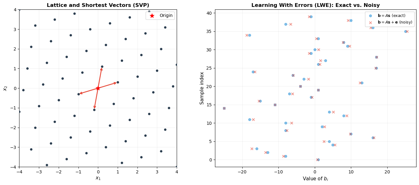
../_images/51331ec8ff0d61e6d325a979a77f52c5ad79b64ceed6a2b5381218ed251bacaa.png

Figure 44.12. Left: A 2D lattice with the shortest nonzero vectors highlighted. The Shortest Vector Problem (SVP) asks to find these vectors, which is computationally hard in high dimensions. Right: The Learning With Errors (LWE) problem – given noisy inner products \(b_i = \langle \mathbf{a}_i, \mathbf{s} \rangle + e_i\), recover the secret \(\mathbf{s}\). The small errors make this problem intractable even for quantum computers.

Why Lattices Are Quantum-Resistant

Unlike factoring and discrete logarithm problems, there is no known quantum algorithm that solves lattice problems (SVP, LWE) in polynomial time. The best known quantum algorithms for lattice problems provide only marginal speedup over classical algorithms, unlike Shor’s exponential speedup against RSA.

44.13 Comprehensive Parameter Summary Table#

The following table consolidates all key parameters across the three NIST standards.

import numpy as np
import matplotlib.pyplot as plt

# --- Comprehensive Summary Table ---
print("=" * 100)
print("NIST POST-QUANTUM CRYPTOGRAPHY STANDARDS: COMPREHENSIVE PARAMETER SUMMARY")
print("=" * 100)

print("\n--- FIPS 203: ML-KEM (Module-Lattice Key Encapsulation Mechanism) ---")
print(f"{'Parameter Set':<20} {'Security':<12} {'PK (B)':<10} {'SK (B)':<10} {'CT (B)':<10} {'SS (B)':<10}")
print("-" * 72)
mlkem_data = [
    ('ML-KEM-512',  'Level 1', 800,  1632, 768,  32),
    ('ML-KEM-768',  'Level 3', 1184, 2400, 1088, 32),
    ('ML-KEM-1024', 'Level 5', 1568, 3168, 1568, 32),
]
for row in mlkem_data:
    print(f"{row[0]:<20} {row[1]:<12} {row[2]:<10} {row[3]:<10} {row[4]:<10} {row[5]:<10}")

print("\n--- FIPS 204: ML-DSA (Module-Lattice Digital Signature Algorithm) ---")
print(f"{'Parameter Set':<20} {'Security':<12} {'PK (B)':<10} {'SK (B)':<10} {'Sig (B)':<10}")
print("-" * 62)
mldsa_data = [
    ('ML-DSA-44', 'Level 2', 1312, 2560, 2420),
    ('ML-DSA-65', 'Level 3', 1952, 4032, 3309),
    ('ML-DSA-87', 'Level 5', 2592, 4896, 4627),
]
for row in mldsa_data:
    print(f"{row[0]:<20} {row[1]:<12} {row[2]:<10} {row[3]:<10} {row[4]:<10}")

print("\n--- FIPS 205: SLH-DSA (Stateless Hash-Based Digital Signature Algorithm) ---")
print(f"{'Parameter Set':<25} {'Security':<12} {'PK (B)':<10} {'SK (B)':<10} {'Sig (B)':<12}")
print("-" * 69)
slhdsa_data = [
    ('SLH-DSA-SHA2-128s', 'Level 1', 32,  64,  7856),
    ('SLH-DSA-SHA2-128f', 'Level 1', 32,  64,  17088),
    ('SLH-DSA-SHA2-192s', 'Level 3', 48,  96,  16224),
    ('SLH-DSA-SHA2-192f', 'Level 3', 48,  96,  35664),
    ('SLH-DSA-SHA2-256s', 'Level 5', 64,  128, 29792),
    ('SLH-DSA-SHA2-256f', 'Level 5', 64,  128, 49856),
]
for row in slhdsa_data:
    print(f"{row[0]:<25} {row[1]:<12} {row[2]:<10} {row[3]:<10} {row[4]:<12}")

print("\nPK = Public Key, SK = Secret Key, CT = Ciphertext, SS = Shared Secret, Sig = Signature")
print("B = bytes")

====================================================================================================
NIST POST-QUANTUM CRYPTOGRAPHY STANDARDS: COMPREHENSIVE PARAMETER SUMMARY
====================================================================================================

--- FIPS 203: ML-KEM (Module-Lattice Key Encapsulation Mechanism) ---
Parameter Set        Security     PK (B)     SK (B)     CT (B)     SS (B)    
------------------------------------------------------------------------
ML-KEM-512           Level 1      800        1632       768        32        
ML-KEM-768           Level 3      1184       2400       1088       32        
ML-KEM-1024          Level 5      1568       3168       1568       32        

--- FIPS 204: ML-DSA (Module-Lattice Digital Signature Algorithm) ---
Parameter Set        Security     PK (B)     SK (B)     Sig (B)   
--------------------------------------------------------------
ML-DSA-44            Level 2      1312       2560       2420      
ML-DSA-65            Level 3      1952       4032       3309      
ML-DSA-87            Level 5      2592       4896       4627      

--- FIPS 205: SLH-DSA (Stateless Hash-Based Digital Signature Algorithm) ---
Parameter Set             Security     PK (B)     SK (B)     Sig (B)     
---------------------------------------------------------------------
SLH-DSA-SHA2-128s         Level 1      32         64         7856        
SLH-DSA-SHA2-128f         Level 1      32         64         17088       
SLH-DSA-SHA2-192s         Level 3      48         96         16224       
SLH-DSA-SHA2-192f         Level 3      48         96         35664       
SLH-DSA-SHA2-256s         Level 5      64         128        29792       
SLH-DSA-SHA2-256f         Level 5      64         128        49856       

PK = Public Key, SK = Secret Key, CT = Ciphertext, SS = Shared Secret, Sig = Signature
B = bytes

44.14 Radar Chart: Multi-Dimensional Comparison#

To capture the multi-faceted trade-offs between PQ algorithms, we visualize several metrics simultaneously using a radar chart.

../_images/119011d374e9862609fa77e63b12f142491244d62b66e1d3af278dac971ffd85.png

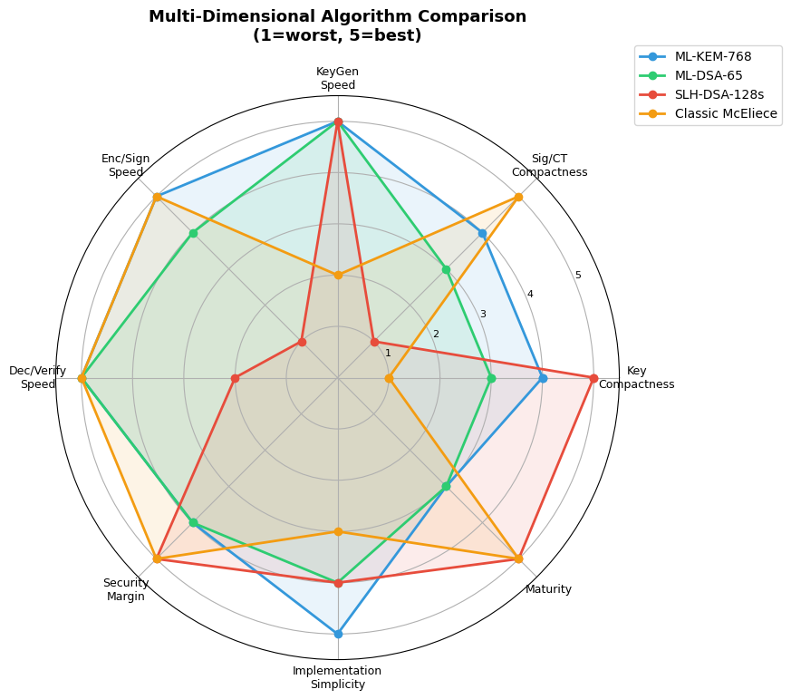
Figure 44.13. Radar chart comparing four post-quantum algorithms across eight dimensions. ML-KEM-768 is the most balanced: compact, fast, and simple to implement. SLH-DSA-128s excels in key compactness and security margin but is extremely slow for signing.

Classic McEliece has the highest maturity (40+ years of cryptanalysis) but impractical key sizes.

44.15 Number Theoretic Transform (NTT) in ML-KEM#

ML-KEM achieves its high performance through the Number Theoretic Transform (NTT), which enables efficient polynomial multiplication in \(\mathbb{Z}_q[X]/(X^{256}+1)\). The NTT is the finite-field analogue of the Fast Fourier Transform.

Show code cell source Hide code cell source

import numpy as np
import matplotlib.pyplot as plt
import math

# --- Simplified NTT Demonstration over Z_q ---
# ML-KEM uses q = 3329 and n = 256
# We demonstrate with small parameters for clarity

q = 3329  # ML-KEM modulus
n = 256   # Polynomial degree

# Find a primitive 2n-th root of unity modulo q
# For q = 3329, a primitive 256th root of unity is 17
zeta = 17

# Verify: zeta^128 should be -1 mod q (i.e., q-1) -- enables negacyclic NTT
zeta_128 = pow(zeta, 128, q)
print(f"ML-KEM Parameters:")
print(f"  q = {q}")
print(f"  n = {n}")
print(f"  Primitive root zeta = {zeta}")
print(f"  q mod 256 = {q % 256} (q \u2261 1 mod 256, so 256th roots of unity exist)")
print(f"  zeta^128 mod q = {zeta_128} (should be {q-1} = -1 mod q)")
print(f"  zeta^256 mod q = {pow(zeta, 256, q)} (should be 1)")
print()

# Demonstrate NTT butterfly operation complexity
# Naive polynomial multiplication: O(n^2)
# NTT-based: O(n log n) for NTT + O(n) pointwise + O(n log n) for inverse NTT

degrees = np.array([16, 32, 64, 128, 256, 512, 1024])
naive_ops = degrees ** 2
ntt_ops = degrees * np.log2(degrees) * 2 + degrees  # 2 NTTs + pointwise mult

fig, ax = plt.subplots(figsize=(10, 6))
ax.semilogy(degrees, naive_ops, 'ro-', linewidth=2, markersize=8, label=r'Naive $O(n^2)$')
ax.semilogy(degrees, ntt_ops, 'bs-', linewidth=2, markersize=8,
            label=r'NTT-based $O(n \log n)$')

# Highlight n=256 (ML-KEM)
ax.axvline(x=256, color='green', linestyle='--', alpha=0.5, label='ML-KEM ($n=256$)')
ax.annotate(f'Speedup at n=256:\n{float(256**2 / (256*8*2+256)):.0f}x',
            xy=(256, 256*8*2+256), xytext=(400, 3000),
            fontsize=10, fontweight='bold',
            arrowprops=dict(arrowstyle='->', color='green'),
            bbox=dict(boxstyle='round', facecolor='#eafaf1'))

ax.set_xlabel('Polynomial Degree $n$', fontsize=12)
ax.set_ylabel('Operations (log scale)', fontsize=12)
ax.set_title('Polynomial Multiplication: Naive vs. NTT-Based',
             fontsize=13, fontweight='bold')
ax.legend(fontsize=11)
ax.grid(True, alpha=0.3)

plt.tight_layout()
plt.savefig('fig_ch44_ntt_complexity.png', dpi=150, bbox_inches='tight')
plt.show()

ML-KEM Parameters:
  q = 3329
  n = 256
  Primitive root zeta = 17
  q mod 256 = 1 (q ≡ 1 mod 256, so 256th roots of unity exist)
  zeta^128 mod q = 3328 (should be 3328 = -1 mod q)
  zeta^256 mod q = 1 (should be 1)

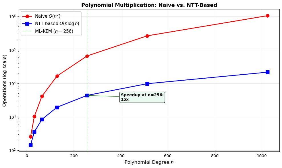
../_images/d35839c20cec940e4a7982c3c88927cf4b50619cd3856f9d33ec4a77a54d7164.png

Figure 44.14. The NTT reduces polynomial multiplication from \(O(n^2)\) to \(O(n \log n)\) operations. At ML-KEM’s \(n = 256\), this provides a roughly 16x speedup, which is a key factor in ML-KEM’s exceptional performance.

44.16 Security Estimation: Core-SVP Hardness#

The security of lattice-based schemes is estimated using the Core-SVP methodology, which measures the cost of the best known lattice reduction attack (typically BKZ with sieving) against the underlying lattice problem.

Show code cell source Hide code cell source

import numpy as np
import matplotlib.pyplot as plt
import math

# --- Core-SVP Security Estimates ---
# Estimated classical and quantum security bits for ML-KEM
# Based on NIST submission documents

param_sets = ['ML-KEM-512', 'ML-KEM-768', 'ML-KEM-1024',
              'ML-DSA-44', 'ML-DSA-65', 'ML-DSA-87']

# Core-SVP security estimates (approximate, from submission docs)
classical_bits = np.array([118, 183, 256, 118, 166, 237])
quantum_bits   = np.array([107, 166, 232, 107, 151, 215])

# NIST target thresholds
nist_targets = {
    'Level 1': 128, 'Level 2': 128, 'Level 3': 192, 'Level 5': 256
}

x = np.arange(len(param_sets))
width = 0.35

fig, ax = plt.subplots(figsize=(12, 6))
bars_c = ax.bar(x - width/2, classical_bits, width, label='Classical Core-SVP',
                color='#2980b9', edgecolor='black', linewidth=0.5)
bars_q = ax.bar(x + width/2, quantum_bits, width, label='Quantum Core-SVP',
                color='#8e44ad', edgecolor='black', linewidth=0.5)

# Add NIST level thresholds
ax.axhline(y=128, color='#e74c3c', linestyle='--', alpha=0.5, label='Level 1/2 target (128)')
ax.axhline(y=192, color='#e67e22', linestyle='--', alpha=0.5, label='Level 3/4 target (192)')
ax.axhline(y=256, color='#27ae60', linestyle='--', alpha=0.5, label='Level 5 target (256)')

# Value labels
for bars in [bars_c, bars_q]:
    for bar in bars:
        height = bar.get_height()
        ax.text(bar.get_x() + bar.get_width()/2, height + 3,
                f'{int(height)}', ha='center', fontsize=9, fontweight='bold')

ax.set_xticks(x)
ax.set_xticklabels(param_sets, fontsize=9, rotation=15)
ax.set_ylabel('Security (bits)', fontsize=12)
ax.set_title('Core-SVP Security Estimates for Lattice-Based NIST Standards',
             fontsize=13, fontweight='bold')
ax.legend(fontsize=9, loc='upper left')
ax.set_ylim(0, 290)
ax.grid(axis='y', alpha=0.3)

plt.tight_layout()
plt.savefig('fig_ch44_coresvp_security.png', dpi=150, bbox_inches='tight')
plt.show()

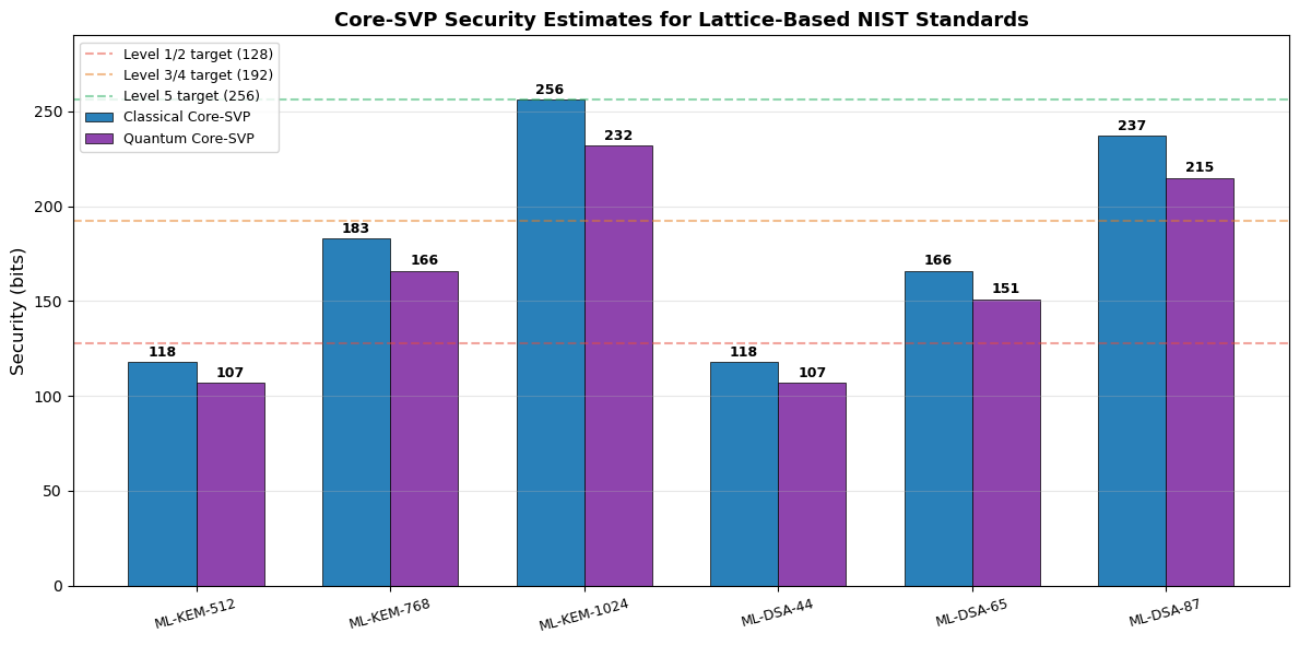
../_images/6a6a2d887565433c58f5889a688a62c2d34aea6986be5ff850d78d4cbc9f1c58.png

Figure 44.15. Core-SVP security estimates for lattice-based NIST standards. The quantum security bits are lower than classical due to Grover-like speedups in lattice sieving. ML-KEM-512 has quantum security slightly below the 128-bit NIST Level 1 target, which is why it is assigned to Level 1. ML-DSA-44, targeting Level 2, also has security estimates in a similar range (the threshold accounts for gate costs).

Security Margin

The gap between the Core-SVP estimate and the NIST target represents the security margin. A larger margin provides more confidence against future cryptanalytic improvements. ML-KEM-768 and ML-KEM-1024 have substantial margins above their respective targets.

44.17 Exercises#

Exercise 44.1: Size Comparison

A TLS 1.3 handshake using ECDHE (P-256) key exchange and ECDSA (P-256) signatures transmits approximately 256 bytes of cryptographic material (two public keys + one signature, ignoring certificates). Calculate the total cryptographic material for a handshake using: (a) ML-KEM-768 + ML-DSA-65, (b) ML-KEM-768 + SLH-DSA-128f, and (c) a hybrid configuration combining both classical and PQ algorithms.

Exercise 44.2: NTT Verification

The ML-KEM modulus is \(q = 3329\) and \(\zeta = 17\) is a primitive 256th root of unity modulo \(q\). Verify computationally that: (a) \(\zeta^{128} \equiv -1 \pmod{q}\) (which enables the negacyclic NTT), (b) \(\zeta^{256} \equiv 1 \pmod{q}\), and (c) \(q \equiv 1 \pmod{256}\), which is necessary for the existence of 256th roots of unity. Also compute the first 8 powers of \(\zeta\) modulo \(q\).

Exercise 44.3: Migration Priority

An organization handles three types of data: (a) real-time video streams (confidentiality needed for minutes), (b) medical records (confidentiality needed for 50+ years), (c) software update signatures (integrity needed until next update). Rank these by PQC migration urgency and explain which NIST standard(s) should protect each. Consider the HNDL threat.

Exercise 44.4: Bandwidth Budget

An IoT sensor sends 100-byte data packets every second over a network with 1 KB/s bandwidth. It must authenticate each packet with a digital signature. Which NIST PQ signature scheme is feasible, if any? Compute the overhead ratio (signature size / data size) for ML-DSA-44, SLH-DSA-128s, and SLH-DSA-128f. Discuss whether batch verification or signature amortization could help.

Exercise 44.5: Security Level Selection

NIST defines five security levels. An organization’s security policy requires protection equivalent to AES-256 (Level 5). List all NIST PQC parameter sets that meet this requirement. Then compute the total key material (public key + secret key) for a system that uses both ML-KEM and ML-DSA at Level 5, and compare it to the equivalent classical configuration (RSA-15360 + ECDSA P-521).

import numpy as np

# --- Exercise 44.1: Solution Sketch ---
print("Exercise 44.1: TLS Handshake Cryptographic Material")
print("=" * 55)

# Classical baseline
ecdhe_pk = 64   # client + server ephemeral public keys
ecdsa_sig = 64  # server signature
ecdsa_pk = 64   # server public key (in certificate)
classical_total = 2 * ecdhe_pk + ecdsa_sig + ecdsa_pk
print(f"\nClassical (ECDHE + ECDSA):")
print(f"  2 x ECDHE PK ({ecdhe_pk} B) + ECDSA sig ({ecdsa_sig} B) + ECDSA PK ({ecdsa_pk} B) = {classical_total} B")

# (a) ML-KEM-768 + ML-DSA-65
mlkem_pk = 1184; mlkem_ct = 1088
mldsa_pk = 1952; mldsa_sig = 3309
pq_a = mlkem_pk + mlkem_ct + mldsa_pk + mldsa_sig
print(f"\n(a) ML-KEM-768 + ML-DSA-65:")
print(f"  KEM PK ({mlkem_pk}) + CT ({mlkem_ct}) + DSA PK ({mldsa_pk}) + Sig ({mldsa_sig}) = {pq_a} B")
print(f"  Overhead vs classical: {float(pq_a / classical_total):.1f}x")

# (b) ML-KEM-768 + SLH-DSA-128f
slh_pk = 32; slh_sig = 17088
pq_b = mlkem_pk + mlkem_ct + slh_pk + slh_sig
print(f"\n(b) ML-KEM-768 + SLH-DSA-128f:")
print(f"  KEM PK ({mlkem_pk}) + CT ({mlkem_ct}) + DSA PK ({slh_pk}) + Sig ({slh_sig}) = {pq_b} B")
print(f"  Overhead vs classical: {float(pq_b / classical_total):.1f}x")

# (c) Hybrid
hybrid = classical_total + pq_a
print(f"\n(c) Hybrid (Classical + PQ-a):")
print(f"  {classical_total} + {pq_a} = {hybrid} B")
print(f"  Overhead vs classical: {float(hybrid / classical_total):.1f}x")

Exercise 44.1: TLS Handshake Cryptographic Material
=======================================================

Classical (ECDHE + ECDSA):
  2 x ECDHE PK (64 B) + ECDSA sig (64 B) + ECDSA PK (64 B) = 256 B

(a) ML-KEM-768 + ML-DSA-65:
  KEM PK (1184) + CT (1088) + DSA PK (1952) + Sig (3309) = 7533 B
  Overhead vs classical: 29.4x

(b) ML-KEM-768 + SLH-DSA-128f:
  KEM PK (1184) + CT (1088) + DSA PK (32) + Sig (17088) = 19392 B
  Overhead vs classical: 75.8x

(c) Hybrid (Classical + PQ-a):
  256 + 7533 = 7789 B
  Overhead vs classical: 30.4x

import numpy as np
import math

# --- Exercise 44.2: Solution Sketch ---
print("Exercise 44.2: NTT Parameter Verification")
print("=" * 45)

q = 3329
zeta = 17
n = 256

# (a) zeta^128 mod q
result_a = pow(zeta, 128, q)
print(f"\n(a) zeta^128 mod q = {result_a}")
print(f"    q - 1 = {q - 1}")
print(f"    zeta^128 = -1 mod q? {result_a == q - 1}")

# (b) zeta^256 mod q
result_b = pow(zeta, 256, q)
print(f"\n(b) zeta^256 mod q = {result_b}")
print(f"    zeta^256 = 1 mod q? {result_b == 1}")

# (c) q mod 256
result_c = q % 256
print(f"\n(c) q mod 256 = {result_c}")
print(f"    q = 1 mod 256? {result_c == 1}")
print(f"    (Verification: 256 * {q // 256} + 1 = {256 * (q // 256) + 1})")

# First 8 powers of zeta
print(f"\nFirst 8 powers of zeta = {zeta} modulo q = {q}:")
for k in range(8):
    print(f"    zeta^{k} = {pow(zeta, k, q)}")

Exercise 44.2: NTT Parameter Verification
=============================================

(a) zeta^128 mod q = 3328
    q - 1 = 3328
    zeta^128 = -1 mod q? True

(b) zeta^256 mod q = 1
    zeta^256 = 1 mod q? True

(c) q mod 256 = 1
    q = 1 mod 256? True
    (Verification: 256 * 13 + 1 = 3329)

First 8 powers of zeta = 17 modulo q = 3329:
    zeta^0 = 1
    zeta^1 = 17
    zeta^2 = 289
    zeta^3 = 1584
    zeta^4 = 296
    zeta^5 = 1703
    zeta^6 = 2319
    zeta^7 = 2804

44.18 Summary#

Key Takeaways

Three NIST standards were finalized in August 2024: ML-KEM (FIPS 203) for key encapsulation, ML-DSA (FIPS 204) for digital signatures, and SLH-DSA (FIPS 205) as a conservative hash-based signature backup.
ML-KEM (based on Kyber) is the recommended KEM. It offers excellent performance (faster than ECDH) with modest key sizes (~1 KB at Level 3). All three parameter sets provide a 32-byte shared secret.
ML-DSA (based on Dilithium) is the recommended signature scheme for most applications. Signatures are 2–5 KB, which is much larger than ECDSA but far more practical than SLH-DSA.
SLH-DSA (based on SPHINCS+) provides the most conservative security: its security relies only on hash function properties. However, signatures are very large (8–50 KB) and signing is slow, limiting its use to applications like firmware signing.
The HNDL threat (Harvest Now, Decrypt Later) makes migration to post-quantum key exchange urgent, even before large-scale quantum computers exist. Data encrypted today with classical algorithms may be stored and decrypted in the future.
Algorithmic diversity is a deliberate strategy: lattice-based (ML-KEM, ML-DSA), hash-based (SLH-DSA), and code-based (HQC, Classic McEliece) schemes ensure resilience against single-family cryptanalytic breakthroughs.
Hybrid deployment – combining classical and post-quantum algorithms – is recommended during the transition period to maintain security even if the PQ algorithm is later found to be flawed.

44.19 Further Reading and References#

Primary Standards#

NIST FIPS 203: Module-Lattice-Based Key-Encapsulation Mechanism Standard (ML-KEM), National Institute of Standards and Technology, August 2024. https://doi.org/10.6028/NIST.FIPS.203
NIST FIPS 204: Module-Lattice-Based Digital Signature Standard (ML-DSA), National Institute of Standards and Technology, August 2024. https://doi.org/10.6028/NIST.FIPS.204
NIST FIPS 205: Stateless Hash-Based Digital Signature Standard (SLH-DSA), National Institute of Standards and Technology, August 2024. https://doi.org/10.6028/NIST.FIPS.205

Background and Analysis#

Avanzi, R. et al.: CRYSTALS-Kyber Algorithm Specifications and Supporting Documentation (Version 3.02), NIST PQC Submission, 2021.
Ducas, L. et al.: CRYSTALS-Dilithium Algorithm Specifications and Supporting Documentation (Version 3.1), NIST PQC Submission, 2021.
Bernstein, D.J. et al.: SPHINCS+ Submission to the NIST Post-Quantum Cryptography Standardization Process, 2022.
NIST: Status Report on the Third Round of the NIST Post-Quantum Cryptography Standardization Process (NISTIR 8413), 2022.
NSA: Commercial National Security Algorithm Suite 2.0 (CNSA 2.0) Cybersecurity Advisory, September 2022.
Shor, P.W.: Polynomial-Time Algorithms for Prime Factorization and Discrete Logarithms on a Quantum Computer, SIAM Journal on Computing, 26(5):1484–1509, 1997.

Chapter 44 of “Elements of Cryptanalysis” – Part XV: Code-Based Frontiers

Next: Chapter 45 provides a synthesis of the entire arc of cryptanalysis, from classical methods to the post-quantum frontier.

Chapter 44: NIST Post-Quantum Cryptography Standards

Contents

Chapter 44: NIST Post-Quantum Cryptography Standards#

44.1 History of the NIST PQC Competition#

Timeline#

44.2 The Finalized Standards#

FIPS 203: ML-KEM (Module-Lattice-Based Key-Encapsulation Mechanism)#

FIPS 204: ML-DSA (Module-Lattice-Based Digital Signature Algorithm)#

FIPS 205: SLH-DSA (Stateless Hash-Based Digital Signature Algorithm)#

44.3 ML-KEM Parameter Details (FIPS 203)#

44.4 ML-DSA Parameter Details (FIPS 204)#

44.5 SLH-DSA Parameter Details (FIPS 205)#

44.6 Additional Candidates: Classic McEliece and HQC#

Classic McEliece#

HQC (Hamming Quasi-Cyclic)#

44.7 Signature Scheme Cross-Comparison#

44.8 Conceptual Performance Benchmarks#

44.9 Security Level Analysis and Quantum Threat Timeline#

44.10 Migration Roadmap#

44.11 Bandwidth Impact Analysis#

44.12 Lattice Parameter Geometry#

44.13 Comprehensive Parameter Summary Table#

44.14 Radar Chart: Multi-Dimensional Comparison#

44.15 Number Theoretic Transform (NTT) in ML-KEM#

44.16 Security Estimation: Core-SVP Hardness#

44.17 Exercises#

44.18 Summary#

44.19 Further Reading and References#

Primary Standards#

Background and Analysis#