
Chapter 34: Gröbner Bases for Cryptanalysis (SageMath)#
Python Version Available
This notebook contains the SageMath implementation. A pure Python/NumPy version is available in Chapter 34: Gröbner Bases for Cryptanalysis.
SageMath provides native Gröbner basis computation via PolynomialRing, ideal(), and .groebner_basis(). The Python version implements Buchberger’s algorithm from scratch (~100+ lines); here, the same computations take 3 lines.
“Every ideal in a polynomial ring over a field has a finite generating set — a Gröbner basis — that makes membership decidable.” — Bruno Buchberger, 1965
In this chapter we introduce Gröbner bases and their computation, focusing on polynomial systems relevant to algebraic cryptanalysis. SageMath’s built-in polynomial algebra makes it possible to compute Gröbner bases efficiently and apply them to solve systems of equations, perform ideal membership tests, and analyze algebraic structures arising in cryptography.
34.1 Historical Context#
Bruno Buchberger introduced Gröbner bases in his 1965 PhD thesis at the University of Innsbruck, naming them after his advisor Wolfgang Gröbner. The algorithm provides a systematic way to solve systems of polynomial equations — a generalization of Gaussian elimination from linear to nonlinear systems.
In the early 2000s, Nicolas Courtois and Josef Pieprzyk proposed using Gröbner bases to attack block ciphers algebraically. Their XSL attack (2002) aimed to express AES as a system of quadratic equations over \(\mathrm{GF}(2)\) and solve them. While the attack hasn’t broken AES in practice, it spurred significant research in algebraic cryptanalysis.
Tip
In the Boolean polynomial ring \(\mathrm{GF}(2)[x_1,\ldots,x_n]/\langle x_i^2 + x_i : i=1,\ldots,n\rangle\), every variable satisfies \(x_i^2 = x_i\) (since we quotient by the field equations). This is the natural algebraic setting for modeling Boolean circuits. Working in this quotient ring, we can always reduce any polynomial to multilinear form (degree at most 1 in each variable), which fundamentally limits the complexity of the polynomial system.
34.2 Formal Definitions#
Definition 34.1 — Polynomial Ideal
An ideal \(I\) in the polynomial ring \(K[x_1, \ldots, x_n]\) is a subset closed under addition and multiplication by ring elements:
Definition 34.2 — Monomial Ordering
A monomial ordering \(\prec\) on \(\{x_1^{a_1} \cdots x_n^{a_n}\}\) is a total order compatible with multiplication. Common orderings:
Lexicographic (lex): compare exponent vectors left-to-right
Graded reverse lex (grevlex): compare total degree first, then reverse lex
Graded lex (grlex): compare total degree first, then lex
Definition 34.3 — Leading Term
For polynomial \(f\) and ordering \(\prec\), the leading term \(\mathrm{LT}(f)\) is the largest monomial appearing in \(f\) with nonzero coefficient.
Definition 34.4 — Gröbner Basis
A finite set \(G = \{g_1, \ldots, g_t\}\) is a Gröbner basis for ideal \(I\) with respect to ordering \(\prec\) if
Equivalently: every \(f \in I\) reduces to zero modulo \(G\).
A Gröbner basis \(B\) for an ideal \(I\) in the ring \(R = K[x_1, \ldots, x_n]\) is a basis which satisfies the condition that the division operation in the ring \(R\) by the elements from the basis \(B\) gives a uniquely determined remainder.
Definition 34.5 — S-Polynomial
The S-polynomial of \(f\) and \(g\) is:
Over \(\mathrm{GF}(2)\), subtraction equals addition.
Theorem 34.1 — Buchberger’s Criterion
\(G\) is a Gröbner basis if and only if \(S(g_i, g_j)\) reduces to zero modulo \(G\) for all pairs \(i \neq j\).
34.3 Gröbner Bases in SageMath#
SageMath provides native support for polynomial ring arithmetic, ideal construction, and Gröbner basis computation. Where the Python version requires 100+ lines to implement Buchberger’s algorithm from scratch, SageMath reduces this to three lines:
R.<x,y,z> = PolynomialRing(QQ)         # 1. Define the ring
I = R.ideal([f1, f2, f3])              # 2. Build the ideal
I.groebner_basis()                      # 3. Compute the basis
Under the hood, SageMath calls the highly optimized Singular library for Gröbner basis computation, which implements F4/F5-style algorithms far more efficient than a naive Buchberger implementation.
Example 1: Basic Gröbner Basis and Monomial Ordering#
Find a Gröbner basis of the ideal \(I = \langle x^2 + y^2 - 1, x + y \rangle \subset \mathbb{Q}[x,y]\).
Remark: The Gröbner basis depends on the chosen monomial ordering. In SageMath, the ordering is determined by the variable declaration order in the polynomial ring.
# Polynomial ring with x > y (default degrevlex ordering)
R.<x,y> = PolynomialRing(Rationals(), 2)
I = R.ideal([x^2 + y^2 - 1, x + y])
print("Groebner basis (x > y):")
I.groebner_basis()
Groebner basis (x > y):
[y^2 - 1/2, x + y]
# Swap variable ordering: y > x
R.<y,x> = PolynomialRing(Rationals(), 2)
I = R.ideal([x^2 + y^2 - 1, x + y])
print("Groebner basis (y > x):")
I.groebner_basis()
Groebner basis (y > x):
[x^2 - 1/2, y + x]
Notice how swapping the variable ordering changes the resulting basis. The ideal is the same, but the leading terms change.
Unique Reduction and Ideal Membership#
Long division with the elements of a Gröbner basis has a unique reduction (remainder). This is the key property that makes Gröbner bases useful: unlike division by an arbitrary generating set, the remainder does not depend on the order in which we perform the divisions.
R.<x,y> = PolynomialRing(Rationals(), 2)
I = R.ideal([x^2 + y^2 - 1, x + y])

# Demonstrate polynomial reduction
aa = x^3 + y^3 - 1
cc = x + y

# Manual reduction steps
print("Original polynomial: ", aa)
step1 = aa - y^2*cc - x^2*cc
print("After reducing by (x+y):", step1)
Original polynomial:  x^3 + y^3 - 1
After reducing by (x+y): -x^2*y - x*y^2 - 1
# Ideal membership test: is x^3 + y^3 in I?
print("Is x^3 + y^3 in I?", (x^3 + y^3) in I)
print("Is x^3 + y^3 - 1 in I?", aa in I)
print("Is aa + 1 in I?", (aa + 1) in I)
Is x^3 + y^3 in I? True
Is x^3 + y^3 - 1 in I? False
Is aa + 1 in I? True
SageMath Advantage — Ideal Membership
The in operator for ideals in SageMath automatically computes the Gröbner basis
and performs division to check if the remainder is zero. In the Python version,
you would need to call reduce_poly(f, G) and check if the result is_zero().
34.4 Solving Polynomial Systems with Varieties#
Let \(V(S) = \{(x_1,\ldots,x_n) \in K^n : \forall_{f \in S}\, f(x_1,\ldots,x_n) = 0\}\) be the set of zeros of the polynomials in \(S\). In other words, this is the set of solutions of the simultaneous system of equations spanned by the basis of the ideal generated by \(S\).
Computation of the Gröbner basis \(B(I)\) of \(I\) simplifies the description of the set \(V(I)\).
Moreover, \(V(I) = V(B(I))\).
Example 2: Solving a Polynomial System#
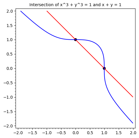
Determine the set \(V(I)\) of the zeros in \(\mathbb{Q}\) of the system \(x^3 + y^3 - 1 = 0\), \(x + y - 1 = 0\) (alternatively, of the ideal \(I = \langle x^3 + y^3 - 1, x + y - 1 \rangle\)).
R.<x,y> = PolynomialRing(Rationals(), 2)
I = R.ideal([x^3 + y^3 - 1, x + y - 1])
gb = I.groebner_basis()
print("Groebner basis:")
for g in gb:
    print(f"  {g}")
Groebner basis:
  y^2 - y
  x + y - 1
The Gröbner basis gives a triangular system: the first polynomial involves only \(y\) (namely \(y^2 - y = 0\)), and the second is \(x + y - 1\). The first equation has two roots: \(y = 0\) and \(y = 1\). The corresponding values of \(x\) are \(x = 1\) and \(x = 0\), respectively.
# Compute rational points directly
V = AffineSpace(R).subscheme(I)
print("Rational solutions:")
V.rational_points()
Rational solutions:
[(0, 1), (1, 0)]
# Visualize the variety
X, Y = var('X', 'Y')

gra = Graphics()
gra += implicit_plot(X + Y - 1, (X, -2, 2), (Y, -2, 2), color='red')
gra += point((0, 1), pointsize=50, color='black') + point((1, 0), pointsize=50, color='black')
gra += implicit_plot(X^3 + Y^3 - 1, (X, -2, 2), (Y, -2, 2))

gra.show(title='Intersection of x^3 + y^3 = 1 and x + y = 1')
Example 3: Lagrange Multipliers via Gröbner Bases#
Find the critical values of \(f(x,y) = x + y^2\) on the ellipse \(x^2 + 2y^2 = 3\).
We use the technique of Lagrange multipliers. Let \(F(x,y,m) = f(x,y) - m(x^2 + 2y^2 - 3)\). We compute the ideal \(I\) in \(K[x,y,m]\) defined by the generators \(\partial_x F\), \(\partial_y F\), \(\partial_m F\).
R.<x,y,m> = PolynomialRing(Rationals(), 3)
F = x + y^2 - m * (x^2 + 2*y^2 - 3)

I = R.ideal([F.derivative(t) for t in [x, y, m]])
print("Groebner basis for Lagrange system:")
for g in I.groebner_basis():
    print(f"  {g}")
Groebner basis for Lagrange system:
  x^2 - x + 6*m - 3
  x*y - y
  y^2 + 1/2*x - 3*m
  x*m - 1/2
  y*m - 1/2*y
  m^2 + 1/12*x - 1/2*m - 1/12
# Decompose V(I) into irreducible components
components = AffineSpace(R).subscheme(I.groebner_basis()).irreducible_components()
print("Irreducible components:")
for c in components:
    print(f"  {c}")
Irreducible components:
  Closed subscheme of Affine Space of dimension 3 over Rational Field defined by:
  2*m - 1,
  y - 1,
  x - 1
  Closed subscheme of Affine Space of dimension 3 over Rational Field defined by:
  2*m - 1,
  y + 1,
  x - 1
  Closed subscheme of Affine Space of dimension 3 over Rational Field defined by:
  y,
  x - 6*m,
  12*m^2 - 1
# Evaluate f at the critical points
critical_points = [(1, 1), (1, -1), (sqrt(3), 0), (-sqrt(3), 0)]

print("Critical values of f(x,y) = x + y^2 on the ellipse:")
for pt in critical_points:
    val = (x + y^2).subs({x: pt[0], y: pt[1]})
    print(f"  f{pt} = {val}")

print("\nMaximum: f(1,1) = f(1,-1) = 2")
print("Minimum: f(-sqrt(3),0) = -sqrt(3)")
Critical values of f(x,y) = x + y^2 on the ellipse:
  f(1, 1) = 2
  f(1, -1) = 2
  f(sqrt(3), 0) = sqrt(3)
  f(-sqrt(3), 0) = -sqrt(3)

Maximum: f(1,1) = f(1,-1) = 2
Minimum: f(-sqrt(3),0) = -sqrt(3)
Observation
Gröbner bases make it possible, through factorization, to determine the
decomposition of \(V(I)\) into irreducible algebraic components. SageMath’s
irreducible_components() method does this automatically.
Example 4: Symbolic Elimination — Power Sum Identity#
Let \(a, b, c\) be complex numbers with known power sums:
Determine \(a^4 + b^4 + c^4\) as an expression in \(m, n, k\).
This is a classic elimination problem: we introduce a new variable \(r = a^4 + b^4 + c^4\) and use a Gröbner basis to eliminate \(a, b, c\), leaving a relation in \(m, n, k, r\).
R.<a,b,c,m,n,k,r> = PolynomialRing(Rationals(), 7)
eq1 = [a + b + c - m,
       a^2 + b^2 + c^2 - n,
       a^3 + b^3 + c^3 - k,
       a^4 + b^4 + c^4 - r]

I = R.ideal(eq1)
gb = I.groebner_basis()

# The first element of the Groebner basis gives the relation involving r
relation = gb[0]
print("Relation from Groebner basis:")
print(f"  {relation}")
Relation from Groebner basis:
  m^4 - 6*m^2*n + 3*n^2 + 8*m*k - 6*r
# Solve for r in terms of m, n, k
solution = (8*k*m + m^4 - 6*m^2*n + 3*n^2) / 6

print("Solution: a^4 + b^4 + c^4 =")
print(f"  (8*k*m + m^4 - 6*m^2*n + 3*n^2) / 6")

# Verify
check = relation.subs({r: solution})
print(f"\nVerification (should be 0): {check}")
Solution: a^4 + b^4 + c^4 =
  (8*k*m + m^4 - 6*m^2*n + 3*n^2) / 6

Verification (should be 0): 0
SageMath vs Python Comparison
The Python version of this chapter implements GF2Polynomial, s_polynomial(),
reduce_poly(), and buchberger() from scratch — over 100 lines of code that
handle monomial representation, orderings, and the full Buchberger loop.
In SageMath, the same work is done by:
R.<x,y,z> = PolynomialRing(QQ)
I = R.ideal([f1, f2, f3])
I.groebner_basis()
SageMath delegates to Singular for computation over \(\mathbb{Q}\), and to
specialized Boolean polynomial ring (BooleanPolynomialRing) for \(\mathrm{GF}(2)\).
These optimized backends handle systems far beyond what a from-scratch
implementation can manage.
34.5 Experiments#
Experiment 1: Solving a System Over GF(2)#
We solve the same polynomial system as the Python chapter, but using SageMath’s
native polynomial ring over \(\mathrm{GF}(2)\). The Python version requires custom
GF2Polynomial objects and a hand-written Buchberger loop; here we use
PolynomialRing(GF(2), ...) directly.
# Define polynomial ring over GF(2)
R.<x0, x1, x2> = PolynomialRing(GF(2), 3)

# System: x0*x1 + x2 + 1 = 0, x0 + x1*x2 = 0, x1 + x2 + 1 = 0
f1 = x0*x1 + x2 + 1
f2 = x0 + x1*x2
f3 = x1 + x2 + 1

print("System over GF(2):")
print(f"  f1: {f1} = 0")
print(f"  f2: {f2} = 0")
print(f"  f3: {f3} = 0")

# Compute Groebner basis
# Add field equations x_i^2 - x_i for GF(2)
field_eqs = [x0^2 + x0, x1^2 + x1, x2^2 + x2]
I = R.ideal([f1, f2, f3] + field_eqs)

gb = I.groebner_basis()
print(f"\nGroebner basis ({len(gb)} elements):")
for g in gb:
    print(f"  {g}")
System over GF(2):
  f1: x0*x1 + x2 + 1 = 0
  f2: x1*x2 + x0 = 0
  f3: x1 + x2 + 1 = 0

Groebner basis (3 elements):
  x0
  x1
  x2 + 1
# Find solutions by enumerating GF(2)^3
solutions = []
for a in GF(2):
    for b in GF(2):
        for c in GF(2):
            if f1(a, b, c) == 0 and f2(a, b, c) == 0 and f3(a, b, c) == 0:
                solutions.append((a, b, c))

print("Solutions (x0, x1, x2):")
for sol in solutions:
    print(f"  {sol}")
Solutions (x0, x1, x2):
  (0, 0, 1)
Experiment 2: Timing Comparison — SageMath vs Brute Force#
We compare the time for Gröbner basis computation vs brute-force enumeration for random quadratic systems over \(\mathrm{GF}(2)\) of increasing size.
import time
# SageMath provides built-in plotting

set_random_seed(42)

def random_quadratic_system_sage(n_vars, n_eqs):
    """Generate a random system of quadratic polynomials over GF(2)."""
    names = [f'x{i}' for i in range(n_vars)]
    R = PolynomialRing(GF(2), names)
    xs = R.gens()
    polys = []
    for _ in range(n_eqs):
        f = R(0)
        # Quadratic terms
        for i in range(n_vars):
            for j in range(i + 1, n_vars):
                if ZZ.random_element(0, 10) < 3:
                    f += xs[i] * xs[j]
        # Linear terms
        for i in range(n_vars):
            if ZZ.random_element(0, 2) == 1:
                f += xs[i]
        # Constant
        if ZZ.random_element(0, 2) == 1:
            f += 1
        polys.append(f)
    return R, polys

def brute_force_gf2(R, polys):
    """Brute-force solve over GF(2)."""
    n = len(R.gens())
    solutions = []
    for val in range(2^n):
        assignment = [(val >> i) & 1 for i in range(n)]
        pt = [GF(2)(a) for a in assignment]
        if all(f(*pt) == 0 for f in polys):
            solutions.append(tuple(pt))
    return solutions

sizes = [3, 4, 5, 6, 7, 8, 9, 10]
bf_times = []
gb_times = []
n_solutions_list = []

print(f"{'n':>4} {'#sols':>8} {'BF time':>12} {'GB time':>12}")
print("=" * 40)

for n in sizes:
    R, system = random_quadratic_system_sage(n, n)

    # Brute force
    t0 = time.time()
    bf_sols = brute_force_gf2(R, system)
    bf_time = time.time() - t0
    bf_times.append(bf_time)

    # Groebner basis
    xs = R.gens()
    field_eqs = [x^2 + x for x in xs]
    t0 = time.time()
    I = R.ideal(system + field_eqs)
    gb = I.groebner_basis()
    gb_time = time.time() - t0
    gb_times.append(gb_time)

    n_solutions_list.append(len(bf_sols))
    print(f"{n:>4} {len(bf_sols):>8} {float(bf_time):>12.4f}s {float(gb_time):>12.4f}s")
   n    #sols      BF time      GB time
========================================
   3        1       0.0001s       0.0014s
   4        2       0.0003s       0.0012s
   5        2       0.0007s       0.0012s
   6        2       0.0016s       0.0015s
   7        2       0.0039s       0.0022s
   8        1       0.0087s       0.0026s
   9        0       0.0190s       0.0042s
10 1 0.0403s 0.0081s
# SageMath plotting for timing comparison

# Left: timing comparison (log scale)
bf_pts = list(zip(sizes, [float(t) for t in bf_times]))
gb_pts = list(zip(sizes, [float(t) for t in gb_times]))

timing_plot = list_plot(bf_pts, plotjoined=True, color='#e74c3c', marker='o',
                        legend_label='Brute Force', thickness=2, scale='semilogy')
timing_plot += list_plot(gb_pts, plotjoined=True, color='#3498db', marker='s',
                         legend_label='Groebner Basis (SageMath)', thickness=2, scale='semilogy')

# Right: solution count bar chart
sol_chart = bar_chart(n_solutions_list, color='#2ecc71')

show(graphics_array([timing_plot, sol_chart], nrows=1, ncols=2), figsize=[12, 5])

Experiment 3: Application to a Simple Cipher#
We express a 2-bit cipher as a polynomial system over \(\mathrm{GF}(2)\) and solve for the key using a Gröbner basis.
Cipher: \(C = S(P \oplus K)\) where \(S\) is a nonlinear S-box on 2 bits: \(S(a,b) = (a \oplus b,\, \overline{a}) = (a + b,\, a + 1)\) over \(\mathrm{GF}(2)\).
# Variables: p0, p1 (plaintext), k0, k1 (key), c0, c1 (ciphertext)
R.<p0, p1, k0, k1, c0, c1> = PolynomialRing(GF(2), 6)

# Cipher equations:
# Internal: u0 = p0 + k0, u1 = p1 + k1
# S-box:   c0 = u0 + u1 = p0 + k0 + p1 + k1
#          c1 = u0 + 1  = p0 + k0 + 1
eq1 = c0 + p0 + k0 + p1 + k1
eq2 = c1 + p0 + k0 + 1

# Known plaintext-ciphertext pair: P = (1, 0), C = (0, 0)
eq_p0 = p0 + 1   # p0 = 1
eq_p1 = p1        # p1 = 0
eq_c0 = c0        # c0 = 0
eq_c1 = c1        # c1 = 0

# Field equations
all_vars = [p0, p1, k0, k1, c0, c1]
field_eqs = [v^2 + v for v in all_vars]

system = [eq1, eq2, eq_p0, eq_p1, eq_c0, eq_c1] + field_eqs

print("Cipher equation system:")
for i, eq in enumerate([eq1, eq2, eq_p0, eq_p1, eq_c0, eq_c1]):
    print(f"  eq{i}: {eq} = 0")

# Solve via Groebner basis
I = R.ideal(system)
gb = I.groebner_basis()

print(f"\nGroebner basis ({len(gb)} elements):")
for g in gb:
    print(f"  {g}")

# Read off the solution
print("\nThe Groebner basis directly gives the unique solution.")
print("Each generator is of the form 'variable + constant', yielding the values.")
Cipher equation system:
  eq0: p0 + p1 + k0 + k1 + c0 = 0
  eq1: p0 + k0 + c1 + 1 = 0
  eq2: p0 + 1 = 0
  eq3: p1 = 0
  eq4: c0 = 0
  eq5: c1 = 0

Groebner basis (6 elements):
  p0 + 1
  p1
  k0
  k1 + 1
  c0
  c1

The Groebner basis directly gives the unique solution.
Each generator is of the form 'variable + constant', yielding the values.
# Brute-force verification
print("Brute-force verification:")
for a in GF(2):
    for b in GF(2):
        for c in GF(2):
            for d in GF(2):
                for e in GF(2):
                    for f in GF(2):
                        pt = [a, b, c, d, e, f]
                        if all(eq(*pt) == 0 for eq in [eq1, eq2, eq_p0, eq_p1, eq_c0, eq_c1]):
                            print(f"  (p0,p1,k0,k1,c0,c1) = {tuple(pt)} -> key = ({c}, {d})")
Brute-force verification:
  (p0,p1,k0,k1,c0,c1) = (1, 0, 0, 1, 0, 0) -> key = (0, 1)
Experiment 4: Equation System Size for an SPN#
We count how many equations and variables are needed to express the Heys 3-round SPN as a polynomial system. This shows that algebraic cryptanalysis is theoretically applicable but computationally limited.
# SageMath provides built-in plotting

def spn_system_size(n_rounds, block_size=16, sbox_size=4, key_size=28):
    """Count variables and equations for an SPN with given parameters."""
    n_sboxes_per_round = block_size // sbox_size

    # Variables
    n_internal = 2 * block_size * n_rounds
    n_total_vars = block_size + block_size + key_size + n_internal

    # Equations
    n_sbox_eqs = 21 * n_sboxes_per_round * n_rounds
    n_xor_eqs = block_size * n_rounds
    n_perm_eqs = block_size * max(0, n_rounds - 1)
    n_final_eqs = block_size

    n_total_eqs = n_sbox_eqs + n_xor_eqs + n_perm_eqs + n_final_eqs

    return n_total_vars, n_total_eqs

rounds_range = range(1, 11)
vars_list = []
eqs_list = []

print(f"{'Rounds':<10} {'Variables':>12} {'Equations':>12} {'Ratio':>8}")
print('=' * 45)

for r in rounds_range:
    v, e = spn_system_size(r)
    vars_list.append(v)
    eqs_list.append(e)
    print(f"{r:<10} {v:>12} {e:>12} {float(e/v):>8.1f}")
Rounds        Variables    Equations    Ratio
=============================================
1                    92          116      1.3
2                   124          232      1.9
3                   156          348      2.2
4                   188          464      2.5
5                   220          580      2.6
6                   252          696      2.8
7                   284          812      2.9
8                   316          928      2.9
9                   348         1044      3.0
10                  380         1160      3.1
# SageMath plotting for SPN system size
vars_pts = list(zip(list(rounds_range), vars_list))
eqs_pts = list(zip(list(rounds_range), eqs_list))

size_plot = list_plot(vars_pts, plotjoined=True, color='#3498db', marker='o',
                      legend_label='Variables', thickness=2)
size_plot += list_plot(eqs_pts, plotjoined=True, color='#e74c3c', marker='s',
                       legend_label='Equations', thickness=2)

# Mark the 3-round Heys SPN
v3, e3 = spn_system_size(3)
size_plot += point2d([(3, v3)], color='black', size=80, zorder=5)
size_plot += text(f'Heys SPN\n({v3} vars, {e3} eqs)', (5, v3 + 50), fontsize=10, color='gray')

size_plot.axes_labels(['Number of Rounds', 'Count'])
show(size_plot, title='Algebraic System Size for SPN Cipher', figsize=[8, 5])
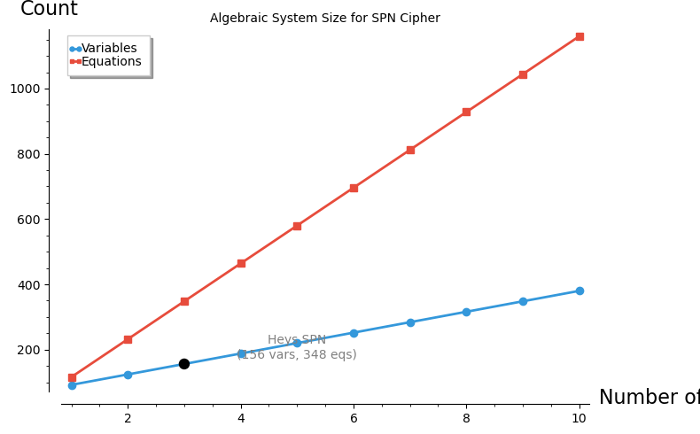
Observation
For the 3-round Heys SPN, the algebraic system has approximately 156 variables and 348 equations. For AES-128 (10 rounds, 128-bit blocks), the system would have thousands of variables and equations — still within reach of theory but far beyond current Gröbner basis solvers for the general case.
Danger
While the number of equations grows linearly with rounds, the complexity of solving the system grows exponentially (or worse) with the number of variables. This is why algebraic attacks have not broken AES in practice, despite the polynomial system being expressible.
Experiment 5: BooleanPolynomialRing for GF(2)#
SageMath provides a specialized BooleanPolynomialRing optimized for \(\mathrm{GF}(2)\)
computations. It uses ZDD (Zero-suppressed Decision Diagrams) internally, which
are much more memory-efficient than the generic polynomial ring for Boolean
systems. The field equations \(x_i^2 = x_i\) are automatically enforced.
# BooleanPolynomialRing automatically enforces x^2 = x
B = BooleanPolynomialRing(3, 'x')
x0, x1, x2 = B.gens()

print("BooleanPolynomialRing demo:")
print(f"  x0^2 = {x0^2}  (automatically reduced to x0)")
print(f"  x0 + x0 = {x0 + x0}  (GF(2): 1+1=0)")
print(f"  x0*x1 + x1*x0 = {x0*x1 + x1*x0}  (cancels over GF(2))")
print()

# Same system as Experiment 1
f1 = x0*x1 + x2 + 1
f2 = x0 + x1*x2
f3 = x1 + x2 + 1

# Groebner basis - no need for field equations!
I = B.ideal([f1, f2, f3])
gb = I.groebner_basis()

print(f"Groebner basis (BooleanPolynomialRing, {len(gb)} elements):")
for g in gb:
    print(f"  {g}")

print("\nNote: field equations x_i^2 + x_i are implicit in BooleanPolynomialRing.")
BooleanPolynomialRing demo:
  x0^2 = x0  (automatically reduced to x0)
  x0 + x0 = 0  (GF(2): 1+1=0)
  x0*x1 + x1*x0 = 0  (cancels over GF(2))

Groebner basis (BooleanPolynomialRing, 3 elements):
  x0
  x1
  x2 + 1

Note: field equations x_i^2 + x_i are implicit in BooleanPolynomialRing.
Implementation Note
SageMath provides two approaches for \(\mathrm{GF}(2)\) polynomial systems:
PolynomialRing(GF(2), ...)— General polynomial ring over \(\mathrm{GF}(2)\). You must manually add field equations \(x_i^2 + x_i\).BooleanPolynomialRing(...)— Specialized ring where \(x_i^2 = x_i\) is automatically enforced. Uses PolyBoRi (Polynomials over Boolean Rings) library with ZDD representation, optimized for cryptanalysis.
For algebraic cryptanalysis, BooleanPolynomialRing is strongly preferred.
Experiment 6: Elimination Ideals for Key Recovery#
One of the most powerful applications of Gröbner bases in cryptanalysis is variable elimination. Given a system involving plaintext, key, and ciphertext variables, we can compute an elimination ideal that removes the key variables, revealing direct relationships between plaintext and ciphertext.
SageMath’s elimination_ideal() makes this straightforward.
# A small SPN-like system: 4-bit state, 4-bit key, 1 round
R.<p0,p1,p2,p3, k0,k1,k2,k3, c0,c1,c2,c3> = PolynomialRing(GF(2), 12)

# Simple round: XOR with key, then a weak 'S-box' (quadratic map)
# u_i = p_i + k_i (key mixing)
# S-box: c0 = u0*u1 + u2, c1 = u1 + u3, c2 = u0*u3, c3 = u2 + u3 + 1
eqs = [
    c0 + (p0+k0)*(p1+k1) + (p2+k2),
    c1 + (p1+k1) + (p3+k3),
    c2 + (p0+k0)*(p3+k3),
    c3 + (p2+k2) + (p3+k3) + 1,
]

# Field equations
all_vars = R.gens()
field_eqs = [v^2 + v for v in all_vars]

I = R.ideal(eqs + field_eqs)

# Eliminate key variables to find plaintext-ciphertext relations
elim = I.elimination_ideal([k0, k1, k2, k3])

print("Relations between plaintext and ciphertext (key eliminated):")
for g in elim.gens():
    if g != 0:
        print(f"  {g} = 0")

if len(elim.gens()) == 1 and elim.gens()[0] == 0:
    print("  No key-independent relations found.")
    print("  (This means the cipher has no trivial structural weakness.)")
Relations between plaintext and ciphertext (key eliminated):
  c3^2 + c3 = 0
  c2^2 + c2 = 0
  c0*c2 + c1*c2 + c2*c3 + c2 = 0
  c1^2 + c1 = 0
  c0^2 + c0 = 0
  p3^2 + p3 = 0
  p2^2 + p2 = 0
  p1^2 + p1 = 0
  p0^2 + p0 = 0
34.6 Exercises#
Exercise 34.1 (Warm-up) Compute \(S(f, g)\) by hand for \(f = x_0 x_1 + x_2\) and \(g = x_0 x_2 + 1\) over \(\mathrm{GF}(2)\) with grevlex ordering. Then verify your answer using SageMath’s polynomial arithmetic.
Hint
\(\mathrm{LT}(f) = x_0 x_1\), \(\mathrm{LT}(g) = x_0 x_2\). \(\mathrm{lcm} = x_0 x_1 x_2\). Quotients: \(x_2\) and \(x_1\). \(S(f,g) = x_2 f + x_1 g\). Compute this in SageMath.
Exercise 34.2 (Applied)
Use SageMath to compute the Gröbner basis of the same ideal under three
different monomial orderings ('degrevlex', 'lex', 'deglex'). Compare
the resulting bases and verify they generate the same ideal.
Hint
Use PolynomialRing(GF(2), 3, 'x', order='lex') to specify the ordering.
For the lex ordering, the Gröbner basis will have a triangular structure
ideal for back-substitution.
Exercise 34.3 (Analysis)
Express the Heys 4-bit S-box as a system of quadratic equations over
\(\mathrm{GF}(2)\). Use BooleanPolynomialRing with 8 variables (4 input, 4 output)
and verify the system has exactly 16 solutions.
Hint
Use AffineSpace(GF(2), 8).subscheme(I).rational_points() or enumerate
all \(2^4\) inputs, compute S-box outputs, and build equations from the
algebraic normal form.
Exercise 34.4 (Theory) Prove that over \(\mathrm{GF}(2)\), any Boolean function on \(n\) variables can be uniquely expressed in algebraic normal form (ANF).
Hint
There are \(2^{2^n}\) Boolean functions on \(n\) variables and \(2^{2^n}\) possible ANF polynomials (each of \(2^n\) monomials is either present or absent). Show that the Möbius transform gives a bijection between truth tables and ANF.
Exercise 34.5 (Challenge)
Using SageMath, model a 2-round version of the Heys SPN cipher as a polynomial
system over \(\mathrm{GF}(2)\). Use elimination_ideal() to identify any
key-independent relationships between plaintext and ciphertext. Discuss
whether these constitute a practical attack.
Hint
Follow the approach from Chapter 35 (SageMath): define the S-box algebraically,
build the full encryption as polynomial expressions, then call
I.elimination_ideal([key variables]). Compare with the approach in
Experiment 6 above.
34.7 Summary#
Concept |
Key Point |
SageMath Function |
|---|---|---|
Polynomial ring |
Base structure for algebraic computations |
|
Ideal |
Set of polynomials closed under ring operations |
|
Gröbner basis |
Generalization of Gaussian elimination to nonlinear systems |
|
Ideal membership |
Test if a polynomial belongs to an ideal |
|
Variety |
Solution set of a polynomial system |
|
Elimination |
Remove variables from a system |
|
Boolean ring |
Optimized ring for \(\mathrm{GF}(2)\) with \(x^2 = x\) built in |
|
Monomial ordering |
Determines basis shape; lex gives triangular form |
|
Tip
Gröbner bases provide the theoretical foundation for algebraic cryptanalysis. In Chapter 35, we will use them to model S-boxes algebraically, and in Chapter 36, we will attempt to attack the Heys SPN using algebraic techniques.
References#
Buchberger, B. (1965). An Algorithm for Finding the Basis Elements of the Residue Class Ring of a Zero-Dimensional Polynomial Ideal. PhD thesis, University of Innsbruck.
Courtois, N. T. and Pieprzyk, J. (2002). Cryptanalysis of Block Ciphers with Overdefined Systems of Equations. ASIACRYPT 2002, LNCS 2501, 267–287.
Faugère, J.-C. (1999). A New Efficient Algorithm for Computing Gröbner Bases (F4). Journal of Pure and Applied Algebra, 139, 61–88.
Bard, G. V. (2009). Algebraic Cryptanalysis. Springer.
Cox, D., Little, J., and O’Shea, D. (2015). Ideals, Varieties, and Algorithms. 4th ed., Springer.
SageMath Documentation. Polynomial Rings. The Sage Developers.