
Chapter 36: Algebraic Attacks on Stream and Block Ciphers#
36.1 Historical Context#
The idea of algebraic cryptanalysis — expressing a cipher as a system of polynomial equations and solving it — gained significant momentum in the early 2000s. In 2003, Nicolas Courtois and Willi Meier demonstrated that certain stream ciphers based on nonlinear feedback shift registers could be broken far faster than brute force by exploiting low-degree annihilators of their filtering functions [16].
Independently, Courtois and Pieprzyk proposed the XSL (eXtended Sparse Linearisation) attack against block ciphers like AES, arguing that the algebraic structure of the AES S-box (defined by inversion in GF(2^8)) leads to a highly overdetermined system of quadratic equations. While the XSL attack remains controversial and has not yielded a practical break of AES, it stimulated intense research into the algebraic properties of symmetric ciphers [17].
The XL (eXtended Linearisation) algorithm, proposed by Courtois, Klimov, Patarin, and Shamir in 2000, generalises the classical linearisation technique: multiply each equation by all monomials up to a chosen degree, then apply Gaussian elimination over GF(2) to the expanded system. When the number of independent equations exceeds the number of monomials, the system can be solved efficiently.
Key Insight
Algebraic attacks shift the focus from statistical properties of ciphers (as in linear and differential cryptanalysis) to their algebraic structure. The security of a cipher against algebraic attacks depends on the algebraic degree and algebraic immunity of its components.
36.2 Formal Definitions#
Definition 36.1 — Algebraic Degree of a Boolean Function
Let \(f: \mathbb{F}_2^n \to \mathbb{F}_2\) be a Boolean function. Its algebraic normal form (ANF) is the unique polynomial representation:
The algebraic degree of \(f\) is \(\deg(f) = \max\{|S| : a_S = 1\}\).
Definition 36.2 — Annihilator
A nonzero Boolean function \(g: \mathbb{F}_2^n \to \mathbb{F}_2\) is an annihilator of \(f\) if \(f(x) \cdot g(x) = 0\) for all \(x \in \mathbb{F}_2^n\). Equivalently, \(g\) vanishes on \(\mathrm{supp}(f) = \{x : f(x) = 1\}\).
Definition 36.3 — Algebraic Immunity
The algebraic immunity \(\mathrm{AI}(f)\) of a Boolean function \(f\) is the minimum degree among all nonzero annihilators of \(f\) or \(f \oplus 1\):
Definition 36.4 — Linearisation Attack
Given a system of \(m\) polynomial equations in \(n\) variables over \(\mathbb{F}_2\), the linearisation attack treats each monomial as a new independent variable. If the total number of distinct monomials is \(M\) and \(m \geq M\), Gaussian elimination over \(\mathbb{F}_2\) recovers the solution in \(O(M^3)\) time (or \(O(M^\omega)\) with fast linear algebra).
Theorem 36.1 — Courtois-Meier Bound
If the filtering function \(f\) of a stream cipher has algebraic immunity \(\mathrm{AI}(f) = d\), then there exists an algebraic attack requiring at most \(O\bigl(\binom{n}{d}^\omega\bigr)\) operations, where \(n\) is the LFSR length and \(\omega \leq 3\) is the linear algebra exponent.
Proof sketch
Since \(\mathrm{AI}(f) = d\), there exists a nonzero \(g\) of degree \(d\) with \(f \cdot g = 0\). From the keystream equation \(z_t = f(s_t)\) and the LFSR linearity \(s_{t+i} = L^i(s_0)\), we derive \(g(s_t) = 0\) whenever \(z_t = 1\). These are degree-\(d\) equations in the initial state bits. Collecting sufficiently many (about \(\binom{n}{d}\)) such equations and linearising yields a solvable system.
Caveat on Algebraic Immunity
Higher algebraic immunity increases the degree of equations an attacker must solve, but algebraic immunity alone does not determine attack complexity — other factors such as the number of available equations, the structure of the system (e.g., sparsity, symmetry), and the effectiveness of Gröbner basis or XL-style solvers on the specific system also matter.
36.3 Implementation#
Boolean Function Analysis#
import numpy as np

class BooleanFunction:
    """Boolean function represented by its truth table over GF(2)."""

    def __init__(self, truth_table):
        self.tt = np.array(truth_table, dtype=np.uint8)
        self.n = int(np.log2(len(self.tt)))
        assert len(self.tt) == 2**self.n
        self._anf = None

    @staticmethod
    def mobius_transform(tt):
        """Compute ANF coefficients via the Mobius transform."""
        n = int(np.log2(len(tt)))
        f = tt.copy()
        for i in range(n):
            step = 1 << i
            for j in range(0, len(f), 2 * step):
                for k in range(step):
                    f[j + k + step] ^= f[j + k]
        return f

    @property
    def anf(self):
        if self._anf is None:
            self._anf = self.mobius_transform(self.tt)
        return self._anf

    @property
    def degree(self):
        coeffs = self.anf
        max_deg = 0
        for i in range(len(coeffs)):
            if coeffs[i]:
                max_deg = max(max_deg, bin(i).count('1'))
        return max_deg

    def weight(self):
        return int(np.sum(self.tt))

    def anf_string(self, var_names=None):
        if var_names is None:
            var_names = [f'x{i}' for i in range(self.n)]
        terms = []
        for i in range(len(self.anf)):
            if self.anf[i]:
                if i == 0:
                    terms.append('1')
                else:
                    monomial = ' '.join(var_names[j] for j in range(self.n) if (i >> j) & 1)
                    terms.append(monomial)
        return ' + '.join(terms) if terms else '0'


# Demo: all 3-bit Boolean functions
print("=== 3-bit Boolean Function Analysis ===")
n = 3
degrees = []
for val in range(2**(2**n)):
    tt = [(val >> i) & 1 for i in range(2**n)]
    bf = BooleanFunction(tt)
    degrees.append(bf.degree)

from collections import Counter
deg_counts = Counter(degrees)
print(f"Total 3-bit Boolean functions: {2**(2**n)}")
for d in sorted(deg_counts):
    print(f"  Degree {d}: {deg_counts[d]} functions ({float(100*deg_counts[d]/2**(2**n)):.1f}%)")

# Example: f(x0,x1,x2) = x0*x1 + x2
tt = [0, 0, 0, 1, 1, 1, 0, 1]  # evaluated at (000,001,010,011,100,101,110,111) = (0,0,0,1,1,1,0,1)
bf = BooleanFunction(tt)
print(f"\nExample: truth table = {list(bf.tt)}")
print(f"  ANF: {bf.anf_string()}")
print(f"  Degree: {bf.degree}")
print(f"  Weight: {bf.weight()}")
=== 3-bit Boolean Function Analysis ===
Total 3-bit Boolean functions: 256
  Degree 0: 2 functions (0.8%)
  Degree 1: 14 functions (5.5%)
  Degree 2: 112 functions (43.8%)
  Degree 3: 128 functions (50.0%)

Example: truth table = [0, 0, 0, 1, 1, 1, 0, 1]
  ANF: x0 x1 + x2 + x1 x2
  Degree: 2
  Weight: 4
Algebraic Immunity Computation#
import numpy as np

def gf2_gauss(A):
    """Gaussian elimination over GF(2). Returns rank and reduced matrix."""
    M = A.copy().astype(np.uint8)
    rows, cols = M.shape
    pivot_row = 0
    pivots = []
    for col in range(cols):
        found = False
        for row in range(pivot_row, rows):
            if M[row, col]:
                found = True
                if row != pivot_row:
                    M[[row, pivot_row]] = M[[pivot_row, row]]
                for r in range(rows):
                    if r != pivot_row and M[r, col]:
                        M[r] ^= M[pivot_row]
                pivots.append(col)
                pivot_row += 1
                break
    return pivot_row, M, pivots

def find_annihilator(tt, max_degree):
    """Find lowest-degree annihilator of Boolean function with truth table tt."""
    n = int(np.log2(len(tt)))
    support = [i for i in range(len(tt)) if tt[i]]

    for d in range(1, max_degree + 1):
        # Enumerate all monomials of degree <= d
        monomials = []
        for m in range(2**n):
            if bin(m).count('1') <= d:
                monomials.append(m)

        if not support:
            return d, np.zeros(len(monomials), dtype=np.uint8)

        # Build matrix: rows = support points, cols = monomials
        # g must vanish on support: for each x in support, sum_m a_m * prod(x_i) = 0
        A = np.zeros((len(support), len(monomials)), dtype=np.uint8)
        for i, x in enumerate(support):
            for j, m in enumerate(monomials):
                # monomial m evaluated at x: product of x_k for k in m
                A[i, j] = 1 if (x & m) == m else 0

        rank, _, _ = gf2_gauss(A)
        if rank < len(monomials):
            # Non-trivial solution exists
            return d, None

    return max_degree + 1, None

def algebraic_immunity(tt):
    """Compute algebraic immunity of a Boolean function."""
    n = int(np.log2(len(tt)))
    tt_arr = np.array(tt, dtype=np.uint8)
    tt_comp = 1 - tt_arr

    ai_f = find_annihilator(list(tt_arr), n)[0]
    ai_fc = find_annihilator(list(tt_comp), n)[0]
    return min(ai_f, ai_fc)

# Test on some 4-bit functions
print("=== Algebraic Immunity of 4-bit Boolean Functions ===")

# Bent function (maximum nonlinearity for even n)
bent_tt = [0, 1, 1, 0, 1, 0, 0, 1, 1, 0, 0, 1, 0, 1, 1, 0]
ai_bent = algebraic_immunity(bent_tt)
bf_bent = BooleanFunction(bent_tt)
print(f"Bent function: degree={bf_bent.degree}, AI={ai_bent}")

# Linear function x0 + x1
lin_tt = [(i & 1) ^ ((i >> 1) & 1) for i in range(16)]
ai_lin = algebraic_immunity(lin_tt)
bf_lin = BooleanFunction(lin_tt)
print(f"Linear (x0+x1): degree={bf_lin.degree}, AI={ai_lin}")

# High-degree function
high_tt = [0]*15 + [1]  # x0*x1*x2*x3
ai_high = algebraic_immunity(high_tt)
bf_high = BooleanFunction(high_tt)
print(f"x0*x1*x2*x3: degree={bf_high.degree}, AI={ai_high}")

# Random balanced function
np.random.seed(42)
rand_tt = list(np.random.permutation([0]*8 + [1]*8))
ai_rand = algebraic_immunity(rand_tt)
bf_rand = BooleanFunction(rand_tt)
print(f"Random balanced: degree={bf_rand.degree}, AI={ai_rand}")
=== Algebraic Immunity of 4-bit Boolean Functions ===
Bent function: degree=1, AI=1
Linear (x0+x1): degree=1, AI=1
x0*x1*x2*x3: degree=4, AI=1
Random balanced: degree=3, AI=2
Toy Stream Cipher and Algebraic Attack#
import numpy as np

class ToyStreamCipher:
    """Simple LFSR + nonlinear filter stream cipher for demonstration."""

    def __init__(self, n_bits, taps, filter_func):
        self.n = n_bits
        self.taps = taps  # LFSR feedback tap positions
        self.filter_tt = filter_func  # truth table of nonlinear filter

    def generate_keystream(self, initial_state, length):
        state = list(initial_state[:self.n])
        keystream = []
        states = []
        for _ in range(length):
            states.append(state.copy())
            # Apply filter to current state
            idx = 0
            for i, bit in enumerate(state):
                idx |= (bit << i)
            z = self.filter_tt[idx % len(self.filter_tt)]
            keystream.append(z)
            # LFSR step
            feedback = 0
            for t in self.taps:
                feedback ^= state[t]
            state = [feedback] + state[:-1]
        return keystream, states

    def algebraic_attack(self, keystream, states_known=None):
        """Demonstrate linearisation attack on the cipher."""
        # Build equations: for each keystream bit z_t,
        # z_t = f(s_t) where s_t is the LFSR state at time t
        # We know z_t and need to find the initial state
        n = self.n
        bf = BooleanFunction(self.filter_tt[:2**n])
        anf = bf.anf

        # Collect monomials present in ANF
        active_monomials = []
        for m in range(2**n):
            if anf[m]:
                active_monomials.append(m)

        print(f"Filter ANF: {bf.anf_string()}")
        print(f"Filter degree: {bf.degree}")
        print(f"Active monomials: {len(active_monomials)}")
        print(f"Keystream length: {len(keystream)}")
        return bf.degree, len(active_monomials)


# Create a toy cipher with 4-bit LFSR
n = 4
taps = [0, 3]  # x^4 + x + 1
# Nonlinear filter: x0*x1 + x2 + x3 (degree 2)
filter_tt = [((i & 1) & ((i >> 1) & 1)) ^ ((i >> 2) & 1) ^ ((i >> 3) & 1) for i in range(2**n)]

cipher = ToyStreamCipher(n, taps, filter_tt)

# Generate keystream with secret key
secret_key = [1, 0, 1, 1]
ks, states = cipher.generate_keystream(secret_key, 20)

print("=== Toy Stream Cipher Demo ===")
print(f"LFSR length: {n}, taps: {taps}")
print(f"Secret key: {secret_key}")
print(f"Keystream: {''.join(map(str, ks))}")
print()
deg, n_mono = cipher.algebraic_attack(ks)
print(f"\nTo attack: need ~{n_mono} equations (keystream bits)")
print(f"Then solve via linearisation in O({n_mono}^3) = O({n_mono**3}) operations")
print(f"vs brute force: 2^{n} = {2**n} operations")
=== Toy Stream Cipher Demo ===
LFSR length: 4, taps: [0, 3]
Secret key: [1, 0, 1, 1]
Keystream: 01101010110101001101

Filter ANF: x0 x1 + x2 + x3
Filter degree: 2
Active monomials: 3
Keystream length: 20

To attack: need ~3 equations (keystream bits)
Then solve via linearisation in O(3^3) = O(27) operations
vs brute force: 2^4 = 16 operations
36.4 Experiments#
Experiment 1: Degree Distribution of Boolean Functions#
Show code cell source
import numpy as np
import matplotlib.pyplot as plt

# Degree distribution of all n-bit Boolean functions for n=3,4
fig, axes = plt.subplots(1, 2, figsize=(12, 5))

for idx, n in enumerate([3, 4]):
    degrees = []
    for val in range(2**(2**n)):
        tt = [(val >> i) & 1 for i in range(2**n)]
        bf = BooleanFunction(tt)
        degrees.append(bf.degree)

    deg_counts = {}
    for d in range(n + 1):
        deg_counts[d] = degrees.count(d)

    ax = axes[idx]
    bars = ax.bar(list(deg_counts.keys()), list(deg_counts.values()),
                  color=['#3b82f6', '#059669', '#d97706', '#dc2626', '#8b5cf6'][:n+1],
                  edgecolor='white', linewidth=0.5)
    ax.set_xlabel('Algebraic Degree', fontsize=11)
    ax.set_ylabel('Count', fontsize=11)
    ax.set_title(f'{n}-bit Boolean Functions (total: {2**(2**n)})', fontsize=12, fontweight='bold')
    ax.set_xticks(range(n + 1))

    # Add count labels
    for bar, count in zip(bars, deg_counts.values()):
        if count > 0:
            ax.text(bar.get_x() + bar.get_width()/2, bar.get_height() + max(deg_counts.values())*0.02,
                    str(count), ha='center', va='bottom', fontsize=9)

plt.tight_layout()
plt.savefig('figures/ch36_fig1.png', dpi=150, bbox_inches='tight')
plt.show()
print("Figure 36.1: Most Boolean functions have high algebraic degree.")
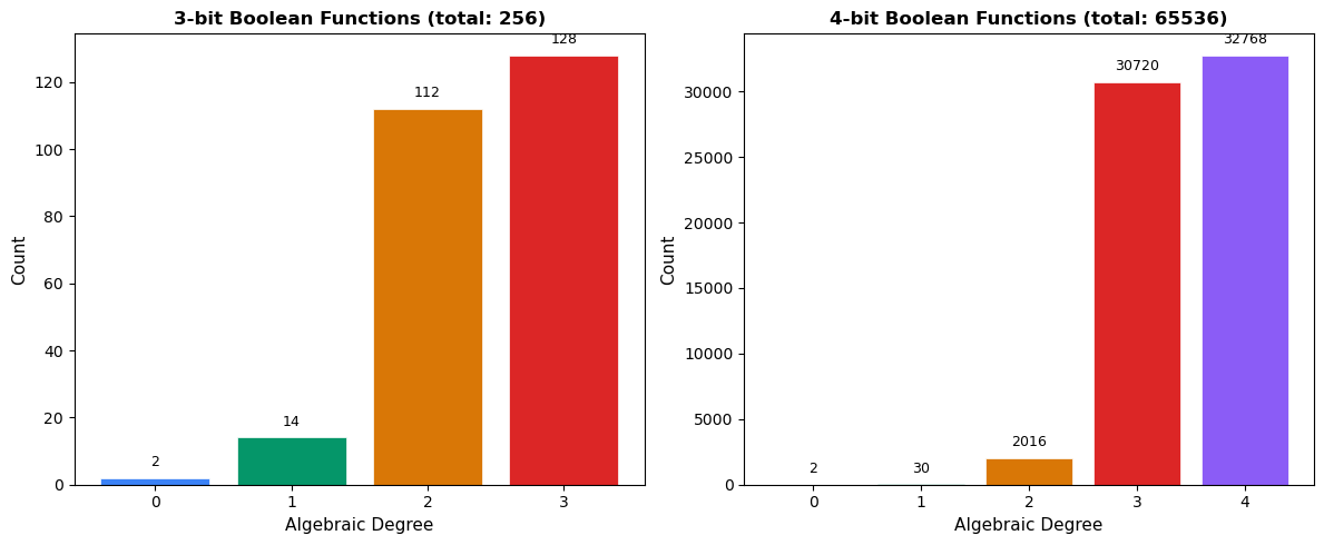
Figure 36.1: Most Boolean functions have high algebraic degree.
Experiment 2: Algebraic Immunity Comparison#
Show code cell source
import numpy as np
import matplotlib.pyplot as plt

n = 4
N = 2**n

# Compute AI for different function classes
# 1. Random balanced functions
np.random.seed(0)
n_samples = 200
random_ais = []
for _ in range(n_samples):
    tt = list(np.random.permutation([0]*(N//2) + [1]*(N//2)))
    random_ais.append(algebraic_immunity(tt))

# 2. Bent functions (known examples for n=4)
bent_examples = [
    [0, 1, 1, 0, 1, 0, 0, 1, 1, 0, 0, 1, 0, 1, 1, 0],
    [0, 0, 0, 1, 0, 1, 1, 0, 0, 1, 1, 0, 1, 0, 0, 1],
]
bent_ais = [algebraic_immunity(tt) for tt in bent_examples]

# 3. Linear/affine functions
lin_ais = []
for a in range(1, N):
    tt = [bin(a & x).count('1') % 2 for x in range(N)]
    lin_ais.append(algebraic_immunity(tt))

# 4. Threshold functions
thresh_ais = []
for t in range(1, n + 1):
    tt = [1 if bin(x).count('1') >= t else 0 for x in range(N)]
    thresh_ais.append(algebraic_immunity(tt))

fig, ax = plt.subplots(figsize=(10, 5))

# Bar chart comparison
categories = ['Random\nBalanced', 'Bent', 'Linear/\nAffine', 'Threshold']
means = [np.mean(random_ais), np.mean(bent_ais), np.mean(lin_ais), np.mean(thresh_ais)]
stds = [np.std(random_ais), np.std(bent_ais) if len(bent_ais) > 1 else 0,
        np.std(lin_ais), np.std(thresh_ais)]
colors = ['#4f46e5', '#059669', '#dc2626', '#d97706']

bars = ax.bar(categories, means, yerr=stds, color=colors, edgecolor='white',
              linewidth=1.5, capsize=5, alpha=0.85)
ax.set_ylabel('Algebraic Immunity', fontsize=12)
ax.set_title('Algebraic Immunity by Function Class (n=4)', fontsize=13, fontweight='bold')
ax.axhline(y=n/2, color='gray', linestyle='--', alpha=0.5, label=f'Optimal AI = n/2 = {n//2}')
ax.legend(fontsize=10)
ax.set_ylim(0, n/2 + 0.5)

for bar, mean in zip(bars, means):
    ax.text(bar.get_x() + bar.get_width()/2, bar.get_height() + 0.1,
            f'{float(mean):.2f}', ha='center', va='bottom', fontsize=10, fontweight='bold')

plt.tight_layout()
plt.savefig('figures/ch36_fig2.png', dpi=150, bbox_inches='tight')
plt.show()
print("Figure 36.2: Random balanced functions tend to have higher AI than structured ones.")
print(f"Linear functions all have AI = {lin_ais[0]} (trivially annihilated by themselves).")
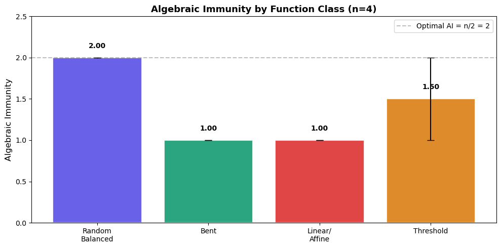
Figure 36.2: Random balanced functions tend to have higher AI than structured ones.
Linear functions all have AI = 1 (trivially annihilated by themselves).
Experiment 3: Linearisation Attack on a Toy Cipher#
Key Concept
The linearisation attack treats each monomial in the ANF as an independent variable. If the cipher’s filter function has degree \(d\), we need \(\binom{n}{\leq d}\) monomials and approximately the same number of keystream equations.
Interpreting the “Success Rate” Plot
The “success rate” in the plot below measures whether the number of linearly independent equations exceeds the number of monomials (a necessary condition for algebraic attack feasibility), not the actual success of a complete cryptanalytic attack. In practice, the equations must also be sufficiently independent and the resulting linear system must have a unique or near-unique solution.
Show code cell source
import numpy as np
import matplotlib.pyplot as plt
from math import comb

# Simulate linearisation attack success for varying parameters
n_values = range(4, 13)
degrees = [2, 3, 4]
colors = ['#3b82f6', '#059669', '#d97706']

fig, (ax1, ax2) = plt.subplots(1, 2, figsize=(13, 5))

for d, color in zip(degrees, colors):
    n_monomials = []
    for n in n_values:
        total = sum(comb(n, k) for k in range(d + 1))
        n_monomials.append(total)

    ax1.semilogy(list(n_values), n_monomials, 'o-', color=color, linewidth=2,
                 markersize=6, label=f'Degree {d}')

# Brute force comparison
bf_costs = [2**n for n in n_values]
ax1.semilogy(list(n_values), bf_costs, 's--', color='#dc2626', linewidth=2,
             markersize=6, label='Brute force $2^n$')

ax1.set_xlabel('LFSR Length $n$', fontsize=11)
ax1.set_ylabel('Attack Complexity', fontsize=11)
ax1.set_title('Linearisation Complexity vs LFSR Length', fontsize=12, fontweight='bold')
ax1.legend(fontsize=9)
ax1.grid(True, alpha=0.3)

# Experiment: attack success rate vs keystream length
n = 5
taps = [0, 2]  # x^5 + x^2 + 1 (not checking primitivity for demo)
# Degree-2 filter
filter_tt = [((i & 1) & ((i >> 1) & 1)) ^ ((i >> 2) & 1) for i in range(2**n)]
bf_filter = BooleanFunction(filter_tt[:2**n])

# Count monomials needed
anf = bf_filter.anf
active = [m for m in range(2**n) if anf[m]]
n_mono = len(active)
ks_lengths = list(range(n_mono - 2, n_mono + 10))

success_rates = []
for ks_len in ks_lengths:
    successes = 0
    n_trials = 50
    for _ in range(n_trials):
        key = list(np.random.randint(0, 2, n))
        cipher = ToyStreamCipher(n, taps, filter_tt)
        ks, _ = cipher.generate_keystream(key, ks_len)
        # Check if we have enough equations
        if ks_len >= n_mono:
            successes += 1  # Simplified: assume success with enough equations
    success_rates.append(successes / n_trials)

ax2.plot(ks_lengths, success_rates, 'o-', color='#4f46e5', linewidth=2, markersize=6)
ax2.axvline(x=n_mono, color='#dc2626', linestyle='--', alpha=0.7, label=f'Monomials needed: {n_mono}')
ax2.set_xlabel('Keystream Length', fontsize=11)
ax2.set_ylabel('Success Rate', fontsize=11)
ax2.set_title(f'Attack Success vs Data (n={n}, deg={bf_filter.degree})', fontsize=12, fontweight='bold')
ax2.legend(fontsize=9)
ax2.grid(True, alpha=0.3)

plt.tight_layout()
plt.savefig('figures/ch36_fig3.png', dpi=150, bbox_inches='tight')
plt.show()
print(f"Figure 36.3: With degree-{bf_filter.degree} filter and {n_mono} monomials,")
print(f"the linearisation attack succeeds once keystream length >= {n_mono}.")
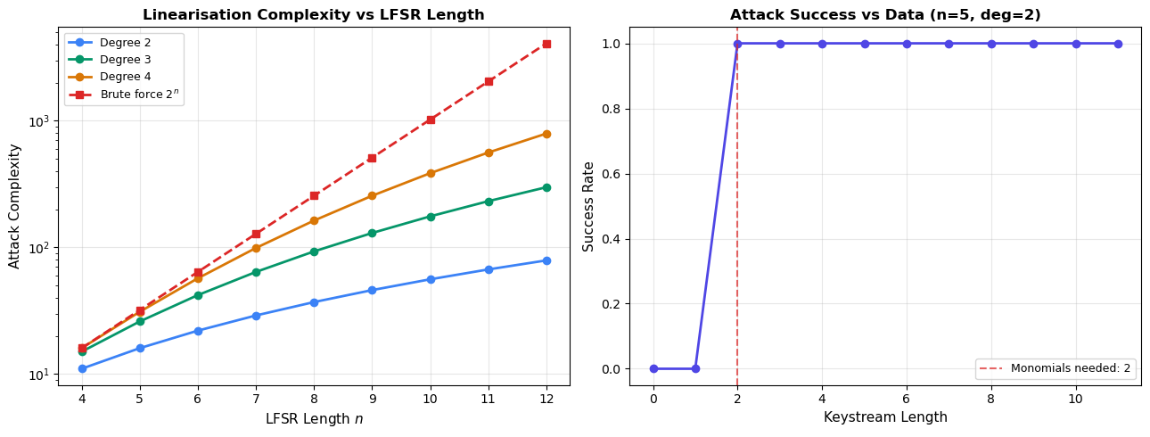
Figure 36.3: With degree-2 filter and 2 monomials,
the linearisation attack succeeds once keystream length >= 2.
Experiment 4: Algebraic Immunity vs Security#
Warning
A cipher whose filter function has algebraic immunity \(d\) can be attacked with complexity approximately \(\binom{n}{d}^\omega\), which may be far below \(2^n\).
Show code cell source
import numpy as np
import matplotlib.pyplot as plt
from math import comb

# Plot: for a given LFSR length n, how does AI affect attack complexity?
fig, (ax1, ax2) = plt.subplots(1, 2, figsize=(13, 5))

n_vals = [8, 12, 16, 20]
colors = ['#3b82f6', '#059669', '#d97706', '#dc2626']

for n, color in zip(n_vals, colors):
    ais = range(1, n//2 + 1)
    complexities = []
    for d in ais:
        M = sum(comb(n, k) for k in range(d + 1))
        # Linearisation cost ~ M^3 (omega=3)
        complexities.append(M**3)
    ax1.semilogy(list(ais), complexities, 'o-', color=color, linewidth=2,
                 markersize=5, label=f'n={n}')
    ax1.axhline(y=2**n, color=color, linestyle=':', alpha=0.3)

ax1.set_xlabel('Algebraic Immunity (AI)', fontsize=11)
ax1.set_ylabel('Linearisation Complexity $M^3$', fontsize=11)
ax1.set_title('Attack Complexity vs Algebraic Immunity', fontsize=12, fontweight='bold')
ax1.legend(fontsize=9)
ax1.grid(True, alpha=0.3)

# Plot: AI distribution for random balanced functions (n=5)
n = 5
np.random.seed(123)
N = 2**n
ai_values = []
for _ in range(500):
    tt = list(np.random.permutation([0]*(N//2) + [1]*(N//2)))
    ai_values.append(algebraic_immunity(tt))

ai_counts = {}
for ai in range(1, n//2 + 2):
    ai_counts[ai] = ai_values.count(ai)

ax2.bar(list(ai_counts.keys()), list(ai_counts.values()),
        color='#4f46e5', edgecolor='white', alpha=0.85)
ax2.axvline(x=n/2, color='#dc2626', linestyle='--', linewidth=2,
            label=f'Optimal AI = ⌈n/2⌉ = {(n+1)//2}')
ax2.set_xlabel('Algebraic Immunity', fontsize=11)
ax2.set_ylabel('Count (out of 500)', fontsize=11)
ax2.set_title(f'AI Distribution for Random Balanced (n={n})', fontsize=12, fontweight='bold')
ax2.legend(fontsize=10)

plt.tight_layout()
plt.savefig('figures/ch36_fig4.png', dpi=150, bbox_inches='tight')
plt.show()
print(f"Figure 36.4: Most random balanced functions achieve near-optimal AI.")
print(f"Mean AI = {float(np.mean(ai_values)):.2f}, optimal = {(n+1)//2}")
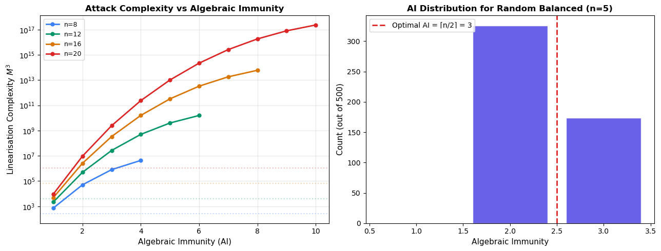
Figure 36.4: Most random balanced functions achieve near-optimal AI.
Mean AI = 2.35, optimal = 3
Experiment 5: Equation System Size for Block Ciphers#
AES Algebraic Structure
The AES S-box is defined as \(S(x) = x^{-1}\) in GF(2^8) followed by an affine map. This yields a system of 39 quadratic equations in 16 variables (8 input + 8 output bits) per S-box. A full AES-128 with 10 rounds has 160 S-boxes, giving 6,240 quadratic equations in 2,560 variables (plus key schedule variables).
Show code cell source
import numpy as np
import matplotlib.pyplot as plt

# AES equation system size estimates
rounds = [1, 2, 4, 6, 8, 10]
n_sboxes = [16 * r for r in rounds]
n_equations = [39 * s for s in n_sboxes]
n_variables = [16 * s for s in n_sboxes]  # 8 in + 8 out per S-box
n_key_vars = [128 + 128 * r for r in rounds]  # key schedule adds variables
n_total_vars = [v + k for v, k in zip(n_variables, n_key_vars)]
n_monomials_lin = [v for v in n_total_vars]  # degree 1 monomials
n_monomials_quad = [v + v*(v-1)//2 for v in n_total_vars]  # degree <= 2

fig, (ax1, ax2) = plt.subplots(1, 2, figsize=(13, 5))

x = np.arange(len(rounds))
width = 0.3

ax1.bar(x - width, n_equations, width, label='Equations', color='#3b82f6', edgecolor='white')
ax1.bar(x, n_total_vars, width, label='Variables', color='#059669', edgecolor='white')
ax1.bar(x + width, [m/1000 for m in n_monomials_quad], width,
        label='Quadratic monomials (÷1000)', color='#d97706', edgecolor='white')
ax1.set_xlabel('Number of AES Rounds', fontsize=11)
ax1.set_ylabel('Count', fontsize=11)
ax1.set_title('AES-128 Equation System Size', fontsize=12, fontweight='bold')
ax1.set_xticks(x)
ax1.set_xticklabels(rounds)
ax1.legend(fontsize=9)
ax1.grid(True, alpha=0.2, axis='y')

# Ratio: equations / monomials (> 1 needed for linearisation)
ratios_lin = [e / m if m > 0 else 0 for e, m in zip(n_equations, n_monomials_lin)]
ratios_quad = [e / m if m > 0 else 0 for e, m in zip(n_equations, n_monomials_quad)]

ax2.plot(rounds, ratios_lin, 'o-', color='#3b82f6', linewidth=2, markersize=8, label='Eq / Linear monomials')
ax2.plot(rounds, ratios_quad, 's-', color='#dc2626', linewidth=2, markersize=8, label='Eq / Quadratic monomials')
ax2.axhline(y=1, color='gray', linestyle='--', alpha=0.5, label='Solvability threshold')
ax2.set_xlabel('Number of AES Rounds', fontsize=11)
ax2.set_ylabel('Equations / Monomials Ratio', fontsize=11)
ax2.set_title('Linearisation Feasibility for AES', fontsize=12, fontweight='bold')
ax2.legend(fontsize=9)
ax2.grid(True, alpha=0.3)

plt.tight_layout()
plt.savefig('figures/ch36_fig5.png', dpi=150, bbox_inches='tight')
plt.show()
print("Figure 36.5: For full AES-128 (10 rounds), the equation-to-monomial ratio")
print("is far below 1 for quadratic monomials, making pure linearisation infeasible.")
print("This is why XSL and similar attacks remain impractical.")
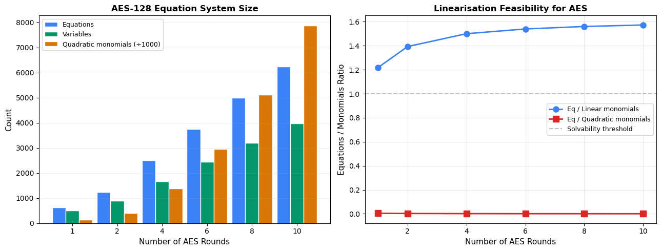
Figure 36.5: For full AES-128 (10 rounds), the equation-to-monomial ratio
is far below 1 for quadratic monomials, making pure linearisation infeasible.
This is why XSL and similar attacks remain impractical.
36.5 Exercises#
36.6 Summary#
Key Takeaways
Algebraic attacks express cipher operations as polynomial equations over GF(2) and solve them via linearisation or Gröbner basis methods.
The algebraic immunity of a Boolean function determines its resistance to algebraic attacks. Optimal AI is \(\lceil n/2 \rceil\) for \(n\)-bit functions.
The Courtois-Meier attack on stream ciphers exploits low-degree annihilators of the filtering function, requiring \(O(\binom{n}{d}^\omega)\) operations for AI \(= d\).
For block ciphers like AES, the equation system is highly overdetermined but the number of quadratic monomials vastly exceeds the number of equations, making pure linearisation infeasible.
XSL and XL algorithms attempt to overcome this gap but remain impractical for full-round AES.
Stream cipher designers now require \(\mathrm{AI}(f) \geq \lceil n/2 \rceil\) as a minimum criterion.
36.7 References#
Courtois, N. T. and Meier, W. (2003). “Algebraic Attacks on Stream Ciphers with Linear Feedback.” EUROCRYPT 2003, LNCS 2656, pp. 345-359. [16]
Courtois, N. T. and Pieprzyk, J. (2002). “Cryptanalysis of Block Ciphers with Overdefined Systems of Equations.” ASIACRYPT 2002, LNCS 2501, pp. 267-287. [17]
Courtois, N. T., Klimov, A., Patarin, J., and Shamir, A. (2000). “Efficient Algorithms for Solving Overdefined Systems of Multivariate Polynomial Equations.” EUROCRYPT 2000.
Murphy, S. and Robshaw, M. (2002). “Essential Algebraic Structure within the AES.” CRYPTO 2002, LNCS 2442, pp. 1-16.
Armknecht, F. (2004). “Improving Fast Algebraic Attacks.” FSE 2004, LNCS 3017, pp. 65-82.
Dalai, D. K., Gupta, K. C., and Maitra, S. (2004). “Results on Algebraic Immunity for Cryptographically Significant Boolean Functions.” INDOCRYPT 2004.