
Chapter 30: Index Calculus#
30.1 Historical Background: Adleman’s Subexponential Breakthrough#
In 1979, Leonard Adleman introduced the index calculus method for solving the discrete logarithm problem (DLP) in the multiplicative group \((\mathbb{Z}/p\mathbb{Z})^*\) of a prime field. The problem is: given a generator \(g\), a prime \(p\), and a target \(h \equiv g^x \pmod{p}\), find the unknown exponent \(x\).
Prior to Adleman’s work, the best generic algorithms for the DLP – such as baby-step/giant-step (Shanks, 1971) and Pollard’s rho (1978) – ran in \(O(\sqrt{p})\) time, which is fully exponential in the bit-length of \(p\). Adleman’s key insight was that the multiplicative group of a prime field has additional structure that generic group algorithms ignore: every element can be lifted to the integers and factored.
The index calculus strategy has three phases:
Factor base selection. Choose a set \(\mathcal{B} = \{p_1, p_2, \ldots, p_k\}\) of small primes.
Relation collection. Compute powers \(g^r \bmod p\) for random exponents \(r\) and keep those that are \(\mathcal{B}\)-smooth (factorable entirely over \(\mathcal{B}\)). Each such power yields a linear equation in the unknown discrete logarithms \(\log_g p_i \pmod{p-1}\).
Individual logarithm. Express \(h \cdot g^s \bmod p\) as a \(\mathcal{B}\)-smooth number for some offset \(s\), then combine with the solved logarithms from phase 2.
This approach achieves subexponential running time, making it dramatically faster than any generic method for large primes. It is the foundational idea behind all modern attacks on the DLP in prime fields, including the number field sieve variants used in practice today.
30.2 Core Definitions#
30.3 Helper Functions: Smoothness Testing and Modular Arithmetic#
import numpy as np

def sieve_primes(B):
    """Return all primes up to B using the Sieve of Eratosthenes."""
    if B < 2:
        return np.array([], dtype=np.int64)
    is_prime = np.ones(B + 1, dtype=bool)
    is_prime[0] = is_prime[1] = False
    for i in range(2, int(np.sqrt(B)) + 1):
        if is_prime[i]:
            is_prime[i*i::i] = False
    return np.where(is_prime)[0].astype(np.int64)

# Quick test
primes_30 = sieve_primes(30)
print(f"Primes up to 30: {primes_30}")
print(f"Count: {len(primes_30)}")
Primes up to 30: [ 2  3  5  7 11 13 17 19 23 29]
Count: 10
import numpy as np

def is_smooth(n, factor_base):
    """
    Test whether n is smooth over the given factor base.

    Returns (True, exponents) if n factors completely over factor_base,
    or (False, None) otherwise.
    """
    if n <= 0:
        return False, None
    exponents = np.zeros(len(factor_base), dtype=np.int64)
    remaining = int(n)
    for i, p in enumerate(factor_base):
        p = int(p)
        while remaining % p == 0:
            exponents[i] += 1
            remaining //= p
    if remaining == 1:
        return True, exponents
    return False, None

# Test: 360 = 2^3 * 3^2 * 5
fb = sieve_primes(10)  # [2, 3, 5, 7]
smooth, exp = is_smooth(360, fb)
print(f"Factor base: {fb}")
print(f"360 is smooth: {smooth}, exponents: {exp}")
print(f"Verification: {np.prod(fb ** exp)} == 360")

# Test a non-smooth number: 77 = 7 * 11
smooth2, _ = is_smooth(77, fb)
print(f"77 is smooth over {{2,3,5,7}}: {smooth2}")
Factor base: [2 3 5 7]
360 is smooth: True, exponents: [3 2 1 0]
Verification: 360 == 360
77 is smooth over {2,3,5,7}: False
import numpy as np
import math

def extended_gcd(a, b):
    """Extended Euclidean algorithm. Returns (g, x, y) with a*x + b*y = g."""
    if a == 0:
        return b, 0, 1
    g, x1, y1 = extended_gcd(b % a, a)
    return g, y1 - (b // a) * x1, x1

def mod_inverse(a, m):
    """Compute modular inverse of a mod m, or None if it does not exist."""
    a = a % m
    g, x, _ = extended_gcd(a, m)
    if g != 1:
        return None  # No inverse exists
    return x % m

def gauss_elim_mod(A, b, m):
    """
    Solve A @ x = b (mod m) using Gaussian elimination with modular arithmetic.

    Parameters
    ----------
    A : ndarray of shape (n_eq, n_var), integer entries
    b : ndarray of shape (n_eq,), integer entries
    m : modulus (typically p - 1)

    Returns
    -------
    x : ndarray of shape (n_var,) -- a solution mod m, or None if no solution.
    """
    n_eq, n_var = A.shape
    # Build augmented matrix [A | b]
    aug = np.zeros((n_eq, n_var + 1), dtype=np.int64)
    aug[:, :n_var] = A % m
    aug[:, n_var] = b % m

    pivot_row = 0
    pivot_cols = []

    for col in range(n_var):
        if pivot_row >= n_eq:
            break
        # Find a row with an invertible entry in this column
        found = False
        for row in range(pivot_row, n_eq):
            val = int(aug[row, col] % m)
            inv = mod_inverse(val, m)
            if inv is not None:
                # Swap rows
                aug[[pivot_row, row]] = aug[[row, pivot_row]]
                # Scale pivot row
                aug[pivot_row] = (aug[pivot_row] * inv) % m
                # Eliminate column in all other rows
                for r in range(n_eq):
                    if r != pivot_row and aug[r, col] != 0:
                        factor = int(aug[r, col])
                        aug[r] = (aug[r] - factor * aug[pivot_row]) % m
                pivot_cols.append(col)
                pivot_row += 1
                found = True
                break
        # If no invertible pivot found, skip this column

    # Extract solution for pivot variables
    x = np.zeros(n_var, dtype=np.int64)
    for i, col in enumerate(pivot_cols):
        x[col] = int(aug[i, n_var] % m)

    # Verify solution
    residual = (A @ x - b) % m
    if not np.all(residual == 0):
        return None
    return x

# Quick test: solve 3x = 6 (mod 10) => x = 2
A_test = np.array([[3]], dtype=np.int64)
b_test = np.array([6], dtype=np.int64)
sol = gauss_elim_mod(A_test, b_test, 10)
print(f"Solution of 3x = 6 (mod 10): x = {sol}")
print(f"Check: 3 * {sol[0]} mod 10 = {(3 * sol[0]) % 10}")
Solution of 3x = 6 (mod 10): x = [2]
Check: 3 * 2 mod 10 = 6
Implementation Note
The modular Gaussian elimination must handle the fact that \(p - 1\) is not prime in general. When the modulus is composite, not every nonzero element has a modular inverse. Our implementation skips columns where no invertible pivot is found, which means some variables may remain undetermined. In practice, collecting extra relations (more than the factor base size) greatly increases the chance of obtaining a full-rank system.
30.4 The Index#
Calculus Class
import numpy as np
import math

class IndexCalculus:
    """
    Index calculus algorithm for the discrete logarithm problem
    in (Z/pZ)*.

    Given g (generator), p (prime), and h = g^x mod p,
    find x.
    """

    def __init__(self, g, p, bound=None):
        """
        Parameters
        ----------
        g : int -- generator of (Z/pZ)*
        p : int -- prime modulus
        bound : int or None -- smoothness bound (auto-selected if None)
        """
        self.g = int(g)
        self.p = int(p)
        self.order = self.p - 1  # order of the group

        if bound is None:
            # Heuristic: L_p[1/2] ~ exp(sqrt(ln p * ln ln p))
            ln_p = math.log(self.p)
            bound = max(10, int(math.exp(0.5 * math.sqrt(ln_p * math.log(ln_p)))))
        self.bound = bound
        self.factor_base = self._sieve_primes(self.bound)
        self.k = len(self.factor_base)  # factor base size
        self.logs = None  # discrete logs of factor base elements
        self.relations = []  # collected relations

    @staticmethod
    def _sieve_primes(B):
        """Sieve of Eratosthenes up to B."""
        if B < 2:
            return np.array([], dtype=np.int64)
        is_prime = np.ones(B + 1, dtype=bool)
        is_prime[0] = is_prime[1] = False
        for i in range(2, int(np.sqrt(B)) + 1):
            if is_prime[i]:
                is_prime[i*i::i] = False
        return np.where(is_prime)[0].astype(np.int64)

    @staticmethod
    def _is_smooth(n, factor_base):
        """Test smoothness and return exponent vector."""
        if n <= 0:
            return False, None
        exponents = np.zeros(len(factor_base), dtype=np.int64)
        remaining = int(n)
        for i, p in enumerate(factor_base):
            p = int(p)
            while remaining % p == 0:
                exponents[i] += 1
                remaining //= p
        if remaining == 1:
            return True, exponents
        return False, None

    def collect_relations(self, max_tries=None, verbose=False):
        """
        Phase 1: Collect B-smooth relations g^r mod p.

        We need at least k relations (one per factor base element).
        We collect extra relations for robustness.
        """
        target = self.k + 10  # collect extra relations
        if max_tries is None:
            max_tries = target * 200

        self.relations = []
        rng = np.random.default_rng(42)

        for _ in range(max_tries):
            r = int(rng.integers(1, self.order))
            val = pow(self.g, r, self.p)
            smooth, exps = self._is_smooth(val, self.factor_base)
            if smooth:
                self.relations.append((r, exps))
                if verbose and len(self.relations) % 5 == 0:
                    print(f"  Collected {len(self.relations)}/{target} relations")
                if len(self.relations) >= target:
                    break

        if verbose:
            print(f"  Total relations collected: {len(self.relations)} "
                  f"(need >= {self.k})")
        return len(self.relations)

    def solve_system(self, verbose=False):
        """
        Phase 2: Solve the linear system mod (p-1) to find
        log_g(p_i) for each prime p_i in the factor base.
        """
        if len(self.relations) < self.k:
            raise ValueError(
                f"Not enough relations: have {len(self.relations)}, "
                f"need >= {self.k}")

        n_rel = len(self.relations)
        A = np.zeros((n_rel, self.k), dtype=np.int64)
        b = np.zeros(n_rel, dtype=np.int64)

        for i, (r, exps) in enumerate(self.relations):
            A[i, :] = exps
            b[i] = r

        self.relation_matrix = A  # store for visualization
        self.logs = gauss_elim_mod(A, b, self.order)

        if self.logs is None:
            if verbose:
                print("  System solve failed -- try more relations.")
            return False

        if verbose:
            for i in range(min(5, self.k)):
                pi = int(self.factor_base[i])
                li = int(self.logs[i])
                check = pow(self.g, li, self.p)
                print(f"  log_g({pi}) = {li}  "
                      f"(verify: g^{li} mod p = {check}, "
                      f"match: {check == pi})")
        return True

    def compute_log(self, h, max_tries=None, verbose=False):
        """
        Phase 3: Compute log_g(h) using the precomputed factor base logs.

        Find offset s such that h * g^s mod p is B-smooth, then
        log_g(h) = sum(e_i * log_g(p_i)) - s  (mod p-1).
        """
        if self.logs is None:
            raise ValueError("Must call solve_system() first.")

        if max_tries is None:
            max_tries = self.order

        h = int(h) % self.p

        for s in range(max_tries):
            val = (h * pow(self.g, s, self.p)) % self.p
            smooth, exps = self._is_smooth(val, self.factor_base)
            if smooth:
                # log_g(h) + s = sum(e_i * log_g(p_i)) mod (p-1)
                log_h = (int(np.dot(exps, self.logs)) - s) % self.order
                if verbose:
                    print(f"  Found smooth value at offset s = {s}")
                    print(f"  h * g^{s} mod p = {val}")
                    print(f"  Factorization exponents: {exps}")
                    print(f"  Computed log_g(h) = {log_h}")
                return int(log_h)

        raise RuntimeError(
            f"Failed to find smooth value in {max_tries} attempts.")
Algorithm Correctness
Each smooth relation \(g^r \equiv p_1^{e_1} \cdots p_k^{e_k} \pmod{p}\) translates into the linear congruence
With enough such relations (\(\geq k\)), the system is (over)determined and Gaussian elimination mod \(p-1\) recovers the individual logarithms. The correctness of Phase 3 follows from the identity \(\log_g(h \cdot g^s) = \log_g h + s\).
30.5 Experiment 1: Full Index Calculus on a ~20-bit Prime#
import numpy as np
import math

# Choose a ~20-bit prime and a generator
p = 1048583  # prime, approx 2^20
# Verify primality by trial division (sufficient for this size)
def is_prime(n):
    if n < 2:
        return False
    for d in range(2, int(math.isqrt(n)) + 1):
        if n % d == 0:
            return False
    return True

print(f"p = {p}, is_prime: {is_prime(p)}, bit-length: {p.bit_length()}")

# Find a primitive root (generator) by testing candidates
def find_generator(p):
    """Find a primitive root modulo p by checking order."""
    # Factor p-1
    n = p - 1
    factors = []
    temp = n
    for d in range(2, int(math.isqrt(temp)) + 1):
        if temp % d == 0:
            factors.append(d)
            while temp % d == 0:
                temp //= d
    if temp > 1:
        factors.append(temp)

    for g in range(2, p):
        is_gen = True
        for q in factors:
            if pow(g, n // q, p) == 1:
                is_gen = False
                break
        if is_gen:
            return g
    return None

g = find_generator(p)
print(f"Generator g = {g}")

# Set up the DLP instance
rng = np.random.default_rng(2024)
secret_x = int(rng.integers(2, p - 1))
h = pow(g, secret_x, p)
print(f"Secret x = {secret_x}")
print(f"h = g^x mod p = {h}")
p = 1048583, is_prime: True, bit-length: 21
Generator g = 5
Secret x = 253263
h = g^x mod p = 861121
import numpy as np

# Run the full index calculus attack
ic = IndexCalculus(g, p, bound=30)
print(f"Factor base (B={ic.bound}): {ic.factor_base}")
print(f"Factor base size k = {ic.k}")
print()

# Phase 1: Relation collection
print("=== Phase 1: Relation Collection ===")
n_rel = ic.collect_relations(verbose=True)
print(f"Collected {n_rel} relations.")
print()

# Phase 2: Solve for factor base logs
print("=== Phase 2: Linear Algebra ===")
success = ic.solve_system(verbose=True)
print(f"System solved: {success}")
print()

# Phase 3: Compute individual log
print("=== Phase 3: Individual Logarithm ===")
computed_x = ic.compute_log(h, verbose=True)
print()
print(f"Computed x = {computed_x}")
print(f"True x     = {secret_x}")
print(f"Correct: {computed_x == secret_x}")
print(f"Verification: g^(computed_x) mod p = {pow(g, computed_x, p)} == h = {h}")
Factor base (B=30): [ 2  3  5  7 11 13 17 19 23 29]
Factor base size k = 10

=== Phase 1: Relation Collection ===
  Collected 5/20 relations
  Collected 10/20 relations
  Collected 15/20 relations
  Collected 20/20 relations
  Total relations collected: 20 (need >= 10)
Collected 20 relations.

=== Phase 2: Linear Algebra ===
  log_g(2) = 810776  (verify: g^810776 mod p = 2, match: True)
  log_g(3) = 505750  (verify: g^505750 mod p = 3, match: True)
  log_g(5) = 1  (verify: g^1 mod p = 5, match: True)
  log_g(7) = 1011081  (verify: g^1011081 mod p = 7, match: True)
  log_g(11) = 920680  (verify: g^920680 mod p = 11, match: True)
System solved: True

=== Phase 3: Individual Logarithm ===
  Found smooth value at offset s = 126
  h * g^126 mod p = 1001832
  Factorization exponents: [3 1 0 0 0 3 0 1 0 0]
  Computed log_g(h) = 253263

Computed x = 253263
True x     = 253263
Correct: True
Verification: g^(computed_x) mod p = 861121 == h = 861121
Why It Works
The attack above solved a 20-bit DLP in well under a second. A brute-force search would examine up to \(\sim 10^6\) exponents; baby-step/giant-step would require \(\sim 10^3\) steps but \(O(\sqrt{p})\) memory. Index calculus needs only a modest number of smooth relations and a small linear system, making it particularly efficient as \(p\) grows.
30.6 Experiment 2: Relation Collection Analysis#
Show code cell source
import numpy as np
import matplotlib.pyplot as plt
# Analyze how the number of random trials needed to collect k relations
# varies with factor base size.
p_test = 1048583
g_test = find_generator(p_test)
bounds = [10, 15, 20, 30, 40, 50, 70, 100]
fb_sizes = []
trials_needed = []
relations_found = []
for B in bounds:
fb = sieve_primes(B)
k = len(fb)
fb_sizes.append(k)
# Count how many trials to get k+5 relations
target = k + 5
count = 0
found = 0
rng = np.random.default_rng(123)
for trial in range(200000):
r = int(rng.integers(1, p_test - 1))
val = pow(g_test, r, p_test)
smooth, _ = is_smooth(val, fb)
count += 1
if smooth:
found += 1
if found >= target:
break
trials_needed.append(count)
relations_found.append(found)
print(f"B={int(B):3d}: |FB|={int(k):2d}, target={int(target):2d}, "
f"trials={int(count):6d}, found={int(found):2d}")
fig, (ax1, ax2) = plt.subplots(1, 2, figsize=(12, 5))
ax1.plot(bounds, trials_needed, 'bo-', linewidth=2, markersize=8)
ax1.set_xlabel('Smoothness bound B', fontsize=12)
ax1.set_ylabel('Trials to collect k+5 relations', fontsize=12)
ax1.set_title('Trials Needed vs. Smoothness Bound', fontsize=13)
ax1.set_yscale('log')
ax1.grid(True, alpha=0.3)
ax2.plot(fb_sizes, trials_needed, 'rs-', linewidth=2, markersize=8)
ax2.set_xlabel('Factor base size k', fontsize=12)
ax2.set_ylabel('Trials to collect k+5 relations', fontsize=12)
ax2.set_title('Trials Needed vs. Factor Base Size', fontsize=13)
ax2.set_yscale('log')
ax2.grid(True, alpha=0.3)
plt.tight_layout()
plt.savefig('relation_collection_analysis.png', dpi=150, bbox_inches='tight')
plt.show()
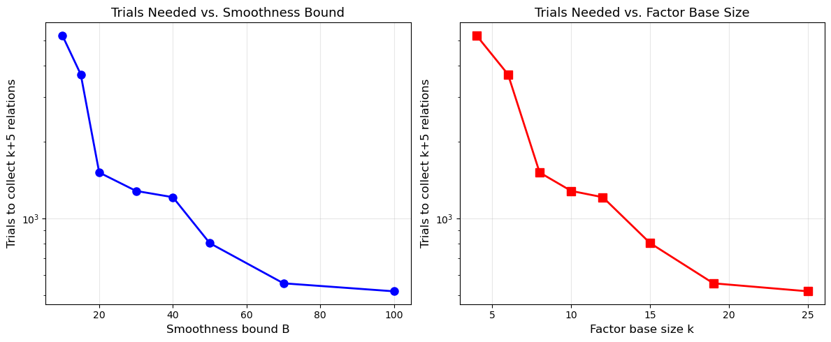
print("\nAs B increases, more numbers are smooth, so fewer trials are needed.")
print("But k also increases, so the linear system grows. The optimal B balances both.")
B= 10: |FB|= 4, target= 9, trials=  5251, found= 9
B= 15: |FB|= 6, target=11, trials=  3688, found=11
B= 20: |FB|= 8, target=13, trials=  1518, found=13
B= 30: |FB|=10, target=15, trials=  1285, found=15
B= 40: |FB|=12, target=17, trials=  1214, found=17
B= 50: |FB|=15, target=20, trials=   801, found=20
B= 70: |FB|=19, target=24, trials=   557, found=24
B=100: |FB|=25, target=30, trials=   518, found=30
As B increases, more numbers are smooth, so fewer trials are needed.
But k also increases, so the linear system grows. The optimal B balances both.
The Smoothness Trade-off
There is a fundamental tension in choosing the smoothness bound \(B\):
Larger \(B\): more numbers are \(B\)-smooth, so relation collection is faster. However, the factor base is larger, so the linear system has more unknowns and the linear algebra phase is slower.
Smaller \(B\): the linear system is compact, but smooth numbers are rarer, making relation collection the bottleneck.
The optimal balance yields the subexponential complexity \(L_p[1/2, c]\).
30.7 Experiment 3: Visualizing the Relation Matrix#
Show code cell source
import numpy as np
import matplotlib.pyplot as plt

# Use the relation matrix from our index calculus instance
A = ic.relation_matrix
n_rel, n_var = A.shape

fig, (ax1, ax2) = plt.subplots(1, 2, figsize=(14, 6))

# Left: sparsity pattern (nonzero entries)
spy_matrix = (A != 0).astype(int)
ax1.imshow(spy_matrix, cmap='Blues', aspect='auto', interpolation='nearest')
ax1.set_xlabel('Factor base index', fontsize=12)
ax1.set_ylabel('Relation index', fontsize=12)
ax1.set_title(f'Sparsity Pattern ({n_rel} x {n_var})\n'
              f'Nonzeros: {np.count_nonzero(A)} / {A.size} '
              f'({float(100*np.count_nonzero(A)/A.size):.1f}%)', fontsize=13)
ax1.set_xticks(range(n_var))
ax1.set_xticklabels([str(int(q)) for q in ic.factor_base], fontsize=9)

# Right: distribution of exponent values
nonzero_vals = A[A > 0]
if len(nonzero_vals) > 0:
    max_exp = int(nonzero_vals.max())
    bins = np.arange(1, max_exp + 2) - 0.5
    ax2.hist(nonzero_vals, bins=bins, color='steelblue',
             edgecolor='white', linewidth=0.8)
    ax2.set_xlabel('Exponent value', fontsize=12)
    ax2.set_ylabel('Frequency', fontsize=12)
    ax2.set_title('Distribution of Nonzero Exponents\nin Relation Matrix',
                  fontsize=13)
    ax2.set_xticks(range(1, max_exp + 1))
ax2.grid(True, alpha=0.3, axis='y')

plt.tight_layout()
plt.savefig('relation_matrix_sparsity.png', dpi=150, bbox_inches='tight')
plt.show()

print(f"Matrix dimensions: {n_rel} relations x {n_var} variables")
print(f"Sparsity: {float(100*(1 - np.count_nonzero(A)/A.size)):.1f}% zeros")
print(f"Small primes (2, 3) appear more frequently because smooth numbers")
print(f"are dominated by small prime factors.")
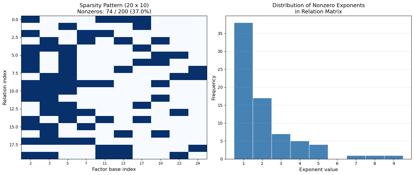
Matrix dimensions: 20 relations x 10 variables
Sparsity: 63.0% zeros
Small primes (2, 3) appear more frequently because smooth numbers
are dominated by small prime factors.
30.8 Experiment 4: BSGS vs. Index Calculus vs. Brute Force#
import numpy as np
import math

def brute_force_log(g, h, p):
    """Solve g^x = h mod p by exhaustive search."""
    power = 1
    for x in range(p - 1):
        if power == h % p:
            return x
        power = (power * g) % p
    return None

def bsgs_log(g, h, p):
    """
    Baby-step/giant-step algorithm for discrete log.
    Solves g^x = h mod p in O(sqrt(p)) time and space.
    """
    n = p - 1  # group order
    m = int(math.isqrt(n)) + 1

    # Baby step: compute g^j mod p for j = 0, ..., m-1
    table = {}
    power = 1
    for j in range(m):
        table[power] = j
        power = (power * g) % p

    # Giant step: g^(-m) mod p
    g_inv_m = pow(g, n - m, p)  # g^(-m) = g^(n-m) mod p

    gamma = h % p
    for i in range(m):
        if gamma in table:
            x = (i * m + table[gamma]) % n
            return x
        gamma = (gamma * g_inv_m) % p
    return None

def index_calculus_log(g, h, p, bound=30):
    """Solve DLP using index calculus."""
    ic_local = IndexCalculus(g, p, bound=bound)
    ic_local.collect_relations()
    if not ic_local.solve_system():
        return None
    return ic_local.compute_log(h)

# Quick verification on a small prime
p_small = 1009  # small prime for testing
g_small = find_generator(p_small)
x_true = 456
h_small = pow(g_small, x_true, p_small)

x_bf = brute_force_log(g_small, h_small, p_small)
x_bs = bsgs_log(g_small, h_small, p_small)

print(f"p = {p_small}, g = {g_small}, h = g^{x_true} = {h_small}")
print(f"Brute force:  x = {x_bf}")
print(f"BSGS:         x = {x_bs}")
print(f"All correct: {pow(g_small, x_bf, p_small) == h_small and pow(g_small, x_bs, p_small) == h_small}")
p = 1009, g = 11, h = g^456 = 185
Brute force:  x = 456
BSGS:         x = 456
All correct: True
Show code cell source
import numpy as np
import matplotlib.pyplot as plt
import math
import time

# Timing comparison across different prime sizes
test_primes = [
    (1009, "~10-bit"),
    (10007, "~14-bit"),
    (100003, "~17-bit"),
    (1048583, "~20-bit"),
]

results = {'prime': [], 'bits': [], 'brute': [], 'bsgs': [], 'ic': []}

for p_val, label in test_primes:
    g_val = find_generator(p_val)
    rng = np.random.default_rng(99)
    x_val = int(rng.integers(2, p_val - 1))
    h_val = pow(g_val, x_val, p_val)
    bits = p_val.bit_length()

    results['prime'].append(p_val)
    results['bits'].append(bits)

    # Brute force (skip if too large)
    if p_val <= 200000:
        t0 = time.perf_counter()
        x_bf = brute_force_log(g_val, h_val, p_val)
        t_bf = time.perf_counter() - t0
        results['brute'].append(t_bf)
    else:
        results['brute'].append(None)

    # BSGS
    t0 = time.perf_counter()
    x_bs = bsgs_log(g_val, h_val, p_val)
    t_bs = time.perf_counter() - t0
    results['bsgs'].append(t_bs)

    # Index calculus
    t0 = time.perf_counter()
    x_ic = index_calculus_log(g_val, h_val, p_val, bound=30)
    t_ic = time.perf_counter() - t0
    results['ic'].append(t_ic)

    print(f"{label} (p={p_val}): "
          f"BF={results['brute'][-1]}, "
          f"BSGS={float(t_bs):.4f}s, "
          f"IC={float(t_ic):.4f}s")

# Plot
fig, ax = plt.subplots(figsize=(10, 6))
bits_arr = np.array(results['bits'])

# Brute force (only for primes where it ran)
bf_mask = [t is not None for t in results['brute']]
bf_bits = bits_arr[bf_mask]
bf_times = [t for t in results['brute'] if t is not None]
if bf_times:
    ax.semilogy(bf_bits, bf_times, 'ro-', linewidth=2, markersize=10,
                label='Brute force $O(p)$')

ax.semilogy(bits_arr, results['bsgs'], 'bs-', linewidth=2, markersize=10,
            label=r'BSGS $O(\sqrt{p})$')
ax.semilogy(bits_arr, results['ic'], 'g^-', linewidth=2, markersize=10,
            label=r'Index calculus $L_p[1/2,c]$')

ax.set_xlabel('Bit-length of p', fontsize=13)
ax.set_ylabel('Time (seconds, log scale)', fontsize=13)
ax.set_title('DLP Solver Comparison: Brute Force vs. BSGS vs. Index Calculus',
             fontsize=14)
ax.legend(fontsize=12)
ax.grid(True, alpha=0.3)
ax.set_xticks(bits_arr)

plt.tight_layout()
plt.savefig('dlp_timing_comparison.png', dpi=150, bbox_inches='tight')
plt.show()
~10-bit (p=1009): BF=6.720796227455139e-05, BSGS=0.0000s, IC=0.0012s
~14-bit (p=10007): BF=0.0006700829835608602, BSGS=0.0000s, IC=0.0012s
~17-bit (p=100003): BF=0.006460999953560531, BSGS=0.0001s, IC=0.0022s
~20-bit (p=1048583): BF=None, BSGS=0.0002s, IC=0.0080s
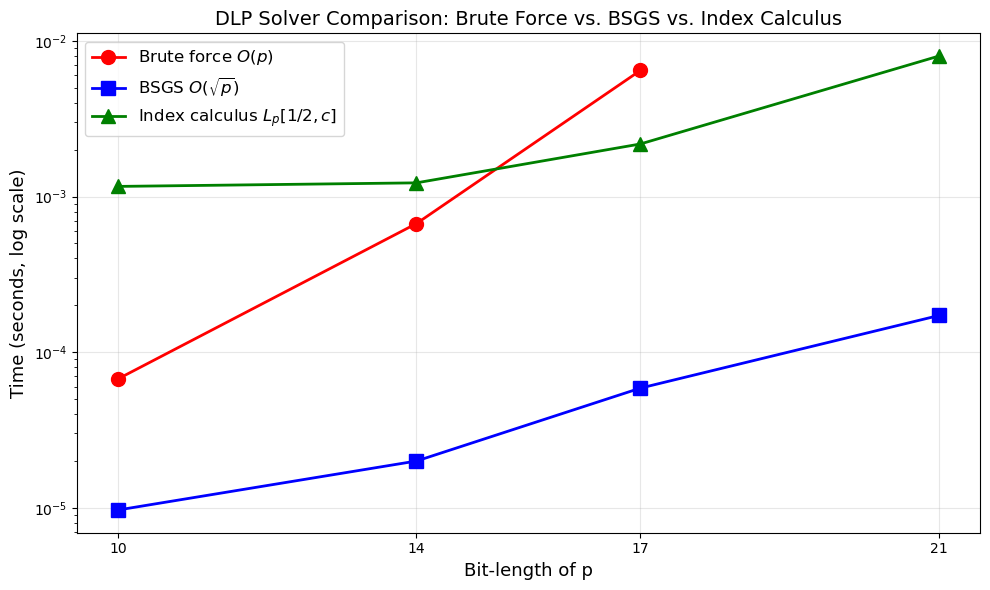
Interpreting the Timing Results
For these small primes, BSGS is typically the fastest algorithm due to low constant factors and the \(O(\sqrt{p})\) complexity. Index calculus incurs overhead from relation collection and linear algebra, which only becomes worthwhile for significantly larger primes (hundreds of bits and beyond).
The advantage of index calculus is asymptotic: its subexponential scaling \(L_p[1/2, c]\) eventually dominates the \(O(p^{1/2})\) scaling of BSGS. For cryptographic-size primes (\(\geq 1024\) bits), index calculus-family algorithms (including the number field sieve) are the only feasible attacks.
30.9 Experiment 5: Smoothness Probability#
Show code cell source
import numpy as np
import matplotlib.pyplot as plt
import math

def estimate_smoothness_prob(p, B, n_samples=50000):
    """Estimate the probability that a random element of (Z/pZ)* is B-smooth."""
    fb = sieve_primes(B)
    rng = np.random.default_rng(42)
    count = 0
    for _ in range(n_samples):
        val = int(rng.integers(1, p))
        smooth, _ = is_smooth(val, fb)
        if smooth:
            count += 1
    return count / n_samples

def dickman_approx(u):
    """
    Rough approximation of the Dickman rho function rho(u).
    For u >= 1, rho(u) ~ u^(-u) gives the probability that
    a random integer n is n^(1/u)-smooth.
    """
    if u <= 1:
        return 1.0
    return u ** (-u)

p_smooth = 1048583
bounds_test = [5, 10, 15, 20, 30, 50, 70, 100, 150, 200]
empirical_probs = []
theoretical_probs = []

for B in bounds_test:
    prob = estimate_smoothness_prob(p_smooth, B, n_samples=30000)
    empirical_probs.append(prob)

    # u = log(p) / log(B)
    u = math.log(p_smooth) / math.log(max(B, 2))
    theoretical_probs.append(dickman_approx(u))

    print(f"B={int(B):4d}: empirical prob = {float(prob):.5f}, "
          f"Dickman approx rho({float(u):.2f}) = {float(dickman_approx(u)):.5f}")

fig, ax = plt.subplots(figsize=(10, 6))
ax.semilogy(bounds_test, empirical_probs, 'bo-', linewidth=2,
            markersize=8, label='Empirical probability')
ax.semilogy(bounds_test, theoretical_probs, 'r--', linewidth=2,
            label=r'Dickman $\rho(u) \approx u^{-u}$')
ax.set_xlabel('Smoothness bound B', fontsize=13)
ax.set_ylabel('Probability of B-smoothness', fontsize=13)
ax.set_title(f'Smoothness Probability for p = {p_smooth} (~20 bits)',
             fontsize=14)
ax.legend(fontsize=12)
ax.grid(True, alpha=0.3)

plt.tight_layout()
plt.savefig('smoothness_probability.png', dpi=150, bbox_inches='tight')
plt.show()
B=   5: empirical prob = 0.00047, Dickman approx rho(8.61) = 0.00000
B=  10: empirical prob = 0.00140, Dickman approx rho(6.02) = 0.00002
B=  15: empirical prob = 0.00450, Dickman approx rho(5.12) = 0.00023
B=  20: empirical prob = 0.00900, Dickman approx rho(4.63) = 0.00083
B=  30: empirical prob = 0.01460, Dickman approx rho(4.08) = 0.00326
B=  50: empirical prob = 0.03293, Dickman approx rho(3.54) = 0.01130
B=  70: empirical prob = 0.04867, Dickman approx rho(3.26) = 0.02109
B= 100: empirical prob = 0.07217, Dickman approx rho(3.01) = 0.03624
B= 150: empirical prob = 0.11047, Dickman approx rho(2.77) = 0.05987
B= 200: empirical prob = 0.14580, Dickman approx rho(2.62) = 0.08073
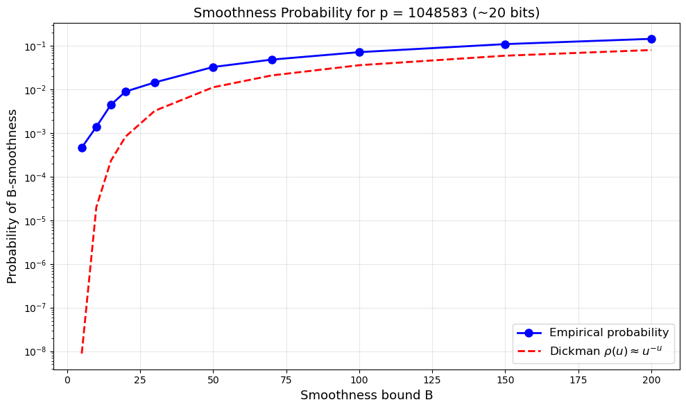
The Dickman Function
The probability that a random integer \(n\) is \(n^{1/u}\)-smooth is given by the Dickman rho function \(\rho(u)\). For \(u = \ln p / \ln B\), the smoothness probability of random elements modulo \(p\) is approximately \(\rho(u)\). The crude approximation \(\rho(u) \approx u^{-u}\) already captures the qualitative behavior: smoothness probability decreases rapidly as the ratio \(\ln p / \ln B\) grows.
30.10 Exercises#
Exercise 30.1. Let \(p = 1009\) and \(g = 11\) (a generator of \((\mathbb{Z}/1009\mathbb{Z})^*\)). Use the factor base \(\mathcal{B} = \{2, 3, 5, 7\}\) and manually verify that \(g^1 = 11\), \(g^2 = 121\), \(g^3 = 1331 \bmod 1009 = 313\). Which of these powers are \(\mathcal{B}\)-smooth? Write out the corresponding linear relations modulo \(p - 1 = 1008\).
Hint
A number is \(\mathcal{B}\)-smooth if it factors completely over \(\{2, 3, 5, 7\}\). Recall \(121 = 11^2\) which is not \(\mathcal{B}\)-smooth. Check \(g^k \bmod p\) for small \(k\) until you find enough smooth values. Each smooth value \(g^k \equiv 2^{a} 3^{b} 5^{c} 7^{d} \pmod{p}\) gives \(k \equiv a \log_g 2 + b \log_g 3 + c \log_g 5 + d \log_g 7 \pmod{1008}\).
Exercise 30.2. Implement a function smoothness_ratio(p, B, N) that
generates \(N\) random integers in \([1, p)\) and returns the fraction that are
\(B\)-smooth. Plot the ratio as a function of \(B\) for \(p = 10^6 + 3\).
At what value of \(B\) is approximately 10% of integers smooth?
Hint
Use the is_smooth function from Section 30.3. Generate random values with
np.random.default_rng().integers(1, p, size=N) and test each. The 10% threshold
can be estimated visually from the plot or by interpolation.
Exercise 30.3. The modular Gaussian elimination in Section 30.3 can fail when the modulus \(m = p - 1\) is composite and a pivot element has no inverse modulo \(m\). Describe a concrete example where this happens (give specific values of \(p\), the factor base, and the relation matrix), and explain how collecting additional relations can help overcome this issue.
Hint
Consider \(p = 13\), so \(m = 12\). The element \(4\) has \(\gcd(4, 12) = 4 \neq 1\), so \(4\) is not invertible mod 12. If a pivot column contains only entries divisible by 4, elimination fails. Extra relations provide alternative rows that may have coprime pivots. Another approach is to work modulo the prime-power factors of \(m\) separately and combine via CRT.
Exercise 30.4. Modify the IndexCalculus class to use sequential scanning
instead of random exponents in the relation collection phase: test \(g^1, g^2, g^3, \ldots\)
in order. Compare the number of smooth values found in the first 10000 powers using
sequential vs. random scanning for \(p = 1048583\) and \(B = 30\). Which approach
finds relations faster, and why?
Hint
Sequential scanning has the advantage that you can maintain a running product
\(c = g^k\) by multiplying by \(g\) at each step (avoiding repeated modular
exponentiation). The distribution of smooth values should be similar in both
cases since \(g\) is a generator and its powers are pseudorandom modulo \(p\).
The old SageMath course used sequential scanning – see the original code
where c *= g in a loop.
Exercise 30.5. The subexponential complexity \(L_p[1/2, c]\) depends on the constant \(c\). For the basic index calculus with optimal smoothness bound, one has \(c = \sqrt{2}\). Compute \(L_p[1/2, \sqrt{2}]\) numerically for \(p\) of bit-lengths \(64, 128, 256, 512, 1024\). Plot these values on a log scale and compare with \(\sqrt{p}\) (the BSGS complexity) and \(p\) (brute-force complexity). At what bit-length does index calculus become faster than BSGS according to this estimate?
Hint
Use the formula \(L_p[1/2, c] = \exp(c \sqrt{\ln p \cdot \ln \ln p})\). For \(p \approx 2^n\), \(\ln p \approx n \ln 2\) and \(\ln \ln p \approx \ln(n \ln 2)\). Plot \(\log_2 L_p\), \(\log_2 \sqrt{p} = n/2\), and \(\log_2 p = n\) on the same axes. The crossover point is where \(L_p < \sqrt{p}\).
30.11 Summary and References#
In this chapter we studied the index calculus algorithm, the first subexponential method for the discrete logarithm problem in prime fields.
Key ideas:
The algorithm exploits the lifting of group elements to the integers, where factorization provides additional algebraic structure unavailable to generic group algorithms.
A factor base of small primes defines the notion of smoothness. Smooth powers of the generator yield linear relations among the discrete logarithms of the factor base elements.
Gaussian elimination modulo \(p - 1\) solves for the base logarithms; individual logarithms follow by expressing the target as a smooth product.
The smoothness bound \(B\) creates a trade-off: larger \(B\) makes smooth numbers more common but increases the linear system size. The optimal balance gives the celebrated \(L_p[1/2, c]\) complexity.
Historical significance:
Adleman’s 1979 algorithm was the first to break the \(O(\sqrt{p})\) barrier for DLP in prime fields.
It inspired a long line of improvements: the Coppersmith-Odlyzko-Schroeppel (COS) algorithm (1986), the Gaussian integer method, and ultimately the number field sieve for DLP, which achieves \(L_p[1/3, c]\) complexity.
These algorithms are the reason that Diffie-Hellman and ElGamal over \((\mathbb{Z}/p\mathbb{Z})^*\) require primes of at least 2048 bits for modern security.
References:
L. M. Adleman, “A subexponential algorithm for the discrete logarithm problem with applications to cryptography,” Proceedings of the 20th Annual IEEE Symposium on Foundations of Computer Science (FOCS), pp. 55–60, 1979.
A. M. Odlyzko, “Discrete logarithms: The past and the future,” Designs, Codes and Cryptography, vol. 19, pp. 129–145, 2000.
D. Coppersmith, A. M. Odlyzko, and R. Schroeppel, “Discrete logarithms in \(GF(p)\),” Algorithmica, vol. 1, pp. 1–15, 1986.
A. J. Menezes, P. C. van Oorschot, and S. A. Vanstone, Handbook of Applied Cryptography, CRC Press, 1996. Chapter 3: Number-Theoretic Reference Problems.