
Chapter 41: ML-KEM (Kyber) – Design and Implementation#
ML-KEM (Module-Lattice-Based Key-Encapsulation Mechanism), formerly known as CRYSTALS-Kyber, is the first post-quantum key encapsulation mechanism standardised by NIST as FIPS 203 (August 2024). Its security rests on the hardness of the Module Learning With Errors (MLWE) problem over polynomial rings.
In this chapter we build a simplified but fully functional ML-KEM implementation from scratch using only NumPy, explore the Number Theoretic Transform (NTT) that makes it efficient, and run experiments comparing the three parameter sets (ML-KEM-512, ML-KEM-768, ML-KEM-1024).
Chapter scope
This is a pedagogical implementation designed for clarity, not production use. A real deployment must use constant-time code, validated randomness, and pass the NIST Known Answer Tests (KATs). For production, use a vetted library such as liboqs or the PQClean reference implementation.
41.1 Historical Context: From Kyber to ML-KEM#
The NIST Post-Quantum Cryptography Competition#
In 2016, NIST launched its Post-Quantum Cryptography (PQC) Standardisation Process in anticipation of large-scale quantum computers that would break RSA, Diffie-Hellman, and elliptic curve cryptography via Shor’s algorithm.
The competition received 82 submissions in Round 1 (2017). After three rounds of public evaluation:
Round |
Year |
Candidates |
|---|---|---|
Round 1 |
2017–2019 |
82 \(\to\) 26 |
Round 2 |
2019–2020 |
26 \(\to\) 7 finalists + 8 alternates |
Round 3 |
2020–2022 |
4 selected for standardisation |
In July 2022, NIST selected CRYSTALS-Kyber as the sole KEM standard and CRYSTALS-Dilithium, FALCON, and SPHINCS+ for digital signatures.
CRYSTALS-Kyber \(\to\) ML-KEM (FIPS 203)#
CRYSTALS-Kyber was designed by a team led by Peter Schwabe, Roberto Avanzi, Joppe Bos, Leo Ducas, Eike Kiltz, Tancrede Lepoint, Vadim Lyubashevsky, John Schanck, Gregor Seiler, and Damien Stehle.
In August 2024, NIST published the final standard as FIPS 203: Module-Lattice-Based Key-Encapsulation Mechanism Standard, officially renaming it ML-KEM.
Why lattices?
Lattice-based cryptography offers:
Quantum resistance: no known quantum algorithm solves lattice problems in polynomial time.
Efficiency: key and ciphertext sizes are moderate (hundreds of bytes to a few KB), and operations are fast thanks to the NTT.
Worst-case to average-case reductions: the security of random instances can be related to worst-case lattice problems (via results of Regev, Lyubashevsky, Peikert, and others).
41.2 Mathematical Foundations#
The Polynomial Ring \(R_q\)#
ML-KEM operates over the polynomial quotient ring:
where \(q = 3329\) is a prime chosen so that \(q \equiv 1 \pmod{256}\) (since \(3329 = 13 \times 256 + 1\)), enabling efficient negacyclic NTT-based multiplication.
Elements of \(R_q\) are polynomials of degree at most 255 with coefficients in \(\{0, 1, \ldots, q-1\}\). Addition is coefficient-wise modulo \(q\). Multiplication is polynomial multiplication modulo both \(q\) and \(x^{256}+1\).
Module-LWE (MLWE) Problem#
Given a uniformly random matrix \(\mathbf{A} \in R_q^{k \times k}\) and a secret vector \(\mathbf{s} \in R_q^k\) with small coefficients, the MLWE problem asks to distinguish:
where \(\mathbf{e}\) is a small error vector and \(\mathbf{u}\) is uniformly random.
The parameter \(k\) determines the security level:
Variant |
\(k\) |
NIST Level |
Classical Security |
|---|---|---|---|
ML-KEM-512 |
2 |
1 (AES-128) |
\(\sim 118\) bits |
ML-KEM-768 |
3 |
3 (AES-192) |
\(\sim 182\) bits |
ML-KEM-1024 |
4 |
5 (AES-256) |
\(\sim 256\) bits |
Centered Binomial Distribution (CBD)#
Secret and error polynomials are sampled from the centered binomial distribution \(\text{CBD}_\eta\): for each coefficient, sample \(2\eta\) bits \(a_1, \ldots, a_\eta, b_1, \ldots, b_\eta\) and compute:
This produces integers in \(\{-\eta, \ldots, \eta\}\) with a binomial distribution centered at zero.
Why CBD instead of discrete Gaussian?
Earlier lattice schemes used discrete Gaussian sampling, which is harder to implement in constant time. The CBD is trivially constant-time (just bit operations) and provides comparable security after parameter adjustment.
41.3 The Number Theoretic Transform (NTT)#
The NTT is the finite-field analogue of the FFT. It converts polynomial multiplication from \(O(n^2)\) to \(O(n \log n)\) operations.
Primitive Root of Unity#
For \(q = 3329\) and \(n = 256\), ML-KEM uses a negacyclic NTT that exploits the factorisation of \(x^{256}+1\) over \(\mathbb{Z}_q\).
The key requirement is a primitive \(256\)th root of unity \(\zeta \in \mathbb{Z}_q\), i.e., an element satisfying \(\zeta^{256} \equiv 1 \pmod{q}\) and \(\zeta^{128} \equiv -1 \pmod{q}\).
The value \(\zeta = 17\) serves this purpose for ML-KEM: \(17^{128} \equiv 3328 \equiv -1 \pmod{3329}\), and therefore \(17^{256} \equiv 1 \pmod{3329}\).
Because \(q \equiv 1 \pmod{256}\), the multiplicative group \(\mathbb{Z}_q^*\) contains elements of order 256, and 17 is one such element.
NTT in ML-KEM#
ML-KEM uses a negacyclic NTT that maps a polynomial \(f(x) \in R_q\) to its NTT representation \(\hat{f}\). The negacyclic NTT factors \(x^{256}+1\) into 128 degree-1 polynomials \(x - \zeta^{2i+1}\) for \(i = 0, \ldots, 127\), so the NTT representation consists of 128 pairs of coefficients (one per degree-1 factor).
The forward NTT uses the Cooley-Tukey butterfly:
The inverse NTT uses the Gentleman-Sande butterfly:
After all layers, each coefficient is multiplied by \(n^{-1} \bmod q\).
Pointwise Multiplication#
In NTT domain, polynomial multiplication reduces to 128 base-case multiplications of degree-1 polynomials, making it very efficient.
Computational advantage
Schoolbook polynomial multiplication over \(R_q\) requires \(256^2 = 65{,}536\) multiplications modulo \(q\). NTT-based multiplication requires only \(256 \cdot \log_2(256) / 2 = 1{,}024\) butterfly operations for the transforms plus 128 base-case multiplications – roughly a 30x speedup in operation count. Note that the measured wall-clock speedup of our pure-Python NTT over schoolbook multiplication may differ from this theoretical ratio due to interpreter overhead.
import numpy as np

# --- Verify fundamental NTT parameters for ML-KEM ---
q = 3329   # The Kyber prime
n = 256    # Polynomial degree
zeta = 17  # Primitive 256th root of unity mod q

# Check that q is prime
def is_prime(p):
    if p < 2:
        return False
    for d in range(2, int(p**0.5) + 1):
        if p % d == 0:
            return False
    return True

print(f'q = {q}')
print(f'q is prime: {is_prime(q)}')
print(f'q mod 256 = {q % 256}  (need q ≡ 1 mod 256 for negacyclic NTT)')
print(f'3329 = 13 * 256 + 1 = {13 * 256 + 1}')
print()

# Verify zeta = 17 is a primitive 256th root of unity
print(f'zeta = {zeta}')
print(f'zeta^128 mod q = {pow(zeta, 128, q)}  (should be {q-1} = -1 mod q)')
print(f'zeta^256 mod q = {pow(zeta, 256, q)}  (should be 1)')
print()

# Check it is primitive (order is exactly 256, not a proper divisor)
is_primitive = True
for d in [1, 2, 4, 8, 16, 32, 64, 128]:
    if pow(zeta, d, q) == 1:
        is_primitive = False
        print(f'  NOT primitive: zeta^{d} = 1')
        break
if is_primitive:
    print(f'zeta = {zeta} is a primitive 256th root of unity mod {q}')
    print(f'  (17^128 ≡ {pow(17, 128, q)} ≡ -1 mod {q}  ✓)')

# Compute n^{-1} mod q (needed for inverse NTT)
n_inv = pow(n, -1, q)
print(f'\nn^{{-1}} mod q = {n_inv}  (verify: {n} * {n_inv} mod {q} = {(n * n_inv) % q})')
q = 3329
q is prime: True
q mod 256 = 1  (need q ≡ 1 mod 256 for negacyclic NTT)
3329 = 13 * 256 + 1 = 3329

zeta = 17
zeta^128 mod q = 3328  (should be 3328 = -1 mod q)
zeta^256 mod q = 1  (should be 1)

zeta = 17 is a primitive 256th root of unity mod 3329
  (17^128 ≡ 3328 ≡ -1 mod 3329  ✓)

n^{-1} mod q = 3316  (verify: 256 * 3316 mod 3329 = 1)
41.4 Implementing the NTT#
We implement the NTT class following the ML-KEM specification (FIPS 203, Algorithm 9 and Algorithm 10). The key design choices:
Bit-reversal of the twiddle factor indices, precomputed as a table.
In-place butterfly operations for memory efficiency.
Base-case multiplication for pointwise products in NTT domain.
import numpy as np

class NTT:
    """Number Theoretic Transform for ML-KEM (Kyber).

    Operates in Z_q[x]/(x^256 + 1) with q=3329, zeta=17 (primitive 256th root of unity).
    Adapted from the CRYSTALS-Kyber reference implementation."""

    def __init__(self, zeta=17, q=3329):
        self.zeta = zeta
        self.q = q
        self.n = 256
        # f = 128^{-1} mod q, used in inverse NTT
        self.ntt_f = pow(128, -1, self.q)
        # Precompute twiddle factors with bit-reversed indices
        self.ntt_zetas = [
            pow(self.zeta, self._bitrev(i, 7), self.q) for i in range(128)
        ]

    @staticmethod
    def _bitrev(i, k):
        """Reverse the lowest k bits of integer i."""
        return int(bin(i & ((1 << k) - 1))[2:].zfill(k)[::-1], 2)

    def forward(self, f):
        """Forward NTT (Cooley-Tukey butterfly, FIPS 203 Algorithm 9)."""
        f_ = list(f)
        i = 1
        length = 128
        while length >= 2:
            start = 0
            while start < 256:
                z = self.ntt_zetas[i]
                i += 1
                for j in range(start, start + length):
                    t = (z * f_[j + length]) % self.q
                    f_[j + length] = (f_[j] - t) % self.q
                    f_[j] = (f_[j] + t) % self.q
                start += 2 * length
            length >>= 1
        return f_

    def inverse(self, f):
        """Inverse NTT (Gentleman-Sande butterfly, FIPS 203 Algorithm 10)."""
        f_ = list(f)
        length = 2
        i = 127
        while length <= 128:
            start = 0
            while start < 256:
                z = self.ntt_zetas[i]
                i -= 1
                for j in range(start, start + length):
                    t = f_[j]
                    f_[j] = (t + f_[j + length]) % self.q
                    f_[j + length] = (z * (f_[j + length] - t)) % self.q
                start += 2 * length
            length <<= 1
        for j in range(256):
            f_[j] = (f_[j] * self.ntt_f) % self.q
        return f_

    def basemul(self, a0, a1, b0, b1, gamma):
        """Base-case multiply of two degree-1 polys mod (x^2 - gamma)."""
        c0 = (a0 * b0 + a1 * b1 * gamma) % self.q
        c1 = (a0 * b1 + a1 * b0) % self.q
        return c0, c1

    def pointwise_multiply(self, f_hat, g_hat):
        """Pointwise multiplication in NTT domain (128 base-case muls)."""
        h = [0] * 256
        for i in range(64):
            z = self.ntt_zetas[64 + i]
            h[4*i], h[4*i+1] = self.basemul(
                f_hat[4*i], f_hat[4*i+1],
                g_hat[4*i], g_hat[4*i+1], z)
            h[4*i+2], h[4*i+3] = self.basemul(
                f_hat[4*i+2], f_hat[4*i+3],
                g_hat[4*i+2], g_hat[4*i+3], (-z) % self.q)
        return h

    def ntt_vector(self, vec):
        """Apply forward NTT to each polynomial in a vector."""
        return [self.forward(poly) for poly in vec]

    def intt_vector(self, vec):
        """Apply inverse NTT to each polynomial in a vector."""
        return [self.inverse(poly) for poly in vec]

# Quick test: forward then inverse should be identity
ntt = NTT()
rng = np.random.default_rng(42)
test_poly = [int(x) for x in rng.integers(0, 3329, size=256)]

ntt_result = ntt.forward(test_poly)
recovered = ntt.inverse(ntt_result)

print('NTT round-trip test:')
print(f'  Original[0:8]:  {test_poly[:8]}')
print(f'  NTT[0:8]:       {ntt_result[:8]}')
print(f'  Recovered[0:8]: {recovered[:8]}')
print(f'  Match: {test_poly == recovered}')
NTT round-trip test:
  Original[0:8]:  [297, 2576, 2179, 1461, 1441, 2858, 286, 2321]
  NTT[0:8]:       [3184, 1311, 322, 728, 858, 2422, 1987, 896]
  Recovered[0:8]: [297, 2576, 2179, 1461, 1441, 2858, 286, 2321]
  Match: True
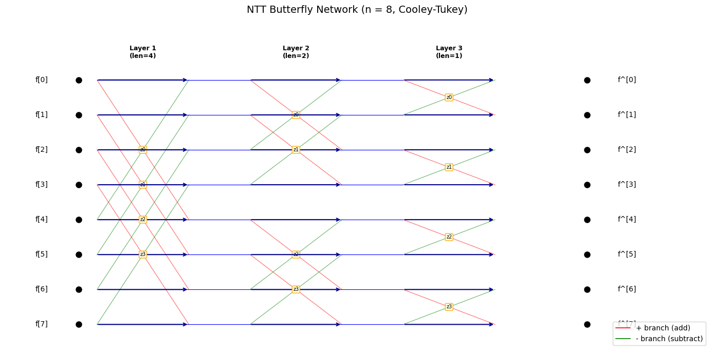
NTT Butterfly Diagram#
The NTT consists of \(\log_2(n) = 8\) layers of butterfly operations. At each layer, pairs of elements are combined using a twiddle factor \(\zeta^{\text{br}(i)}\).
Let us visualise the butterfly structure for a small example (\(n = 8\)) to build intuition before working with the full \(n = 256\) case.
Show code cell source
import numpy as np
import matplotlib.pyplot as plt

fig, ax = plt.subplots(figsize=(14, 7))

n_small = 8
n_layers = int(np.log2(n_small))

# Draw the butterfly network for n=8 NTT
for layer in range(n_layers):
    half_block = n_small >> (layer + 1)
    block_size = 2 * half_block
    x_pos = layer * 2.5

    for block_start in range(0, n_small, block_size):
        for j in range(half_block):
            top = block_start + j
            bot = block_start + j + half_block

            # Lines from previous layer to this butterfly
            if layer > 0:
                ax.plot([x_pos - 2.5, x_pos], [top, top], 'b-', linewidth=0.8)
                ax.plot([x_pos - 2.5, x_pos], [bot, bot], 'b-', linewidth=0.8)

            # Butterfly cross-connections
            ax.annotate('', xy=(x_pos + 1.5, top), xytext=(x_pos, top),
                        arrowprops=dict(arrowstyle='->', color='darkblue', lw=1.5))
            ax.annotate('', xy=(x_pos + 1.5, bot), xytext=(x_pos, bot),
                        arrowprops=dict(arrowstyle='->', color='darkblue', lw=1.5))

            # Cross connections (the butterfly)
            ax.plot([x_pos, x_pos + 1.5], [top, bot], 'r-', linewidth=0.8, alpha=0.6)
            ax.plot([x_pos, x_pos + 1.5], [bot, top], 'g-', linewidth=0.8, alpha=0.6)

            # Twiddle factor label
            br_idx = block_start // block_size * half_block + j
            ax.text(x_pos + 0.75, (top + bot) / 2, f'z{br_idx}',
                    fontsize=7, ha='center', va='center',
                    bbox=dict(boxstyle='round,pad=0.2', facecolor='lightyellow',
                              edgecolor='orange', alpha=0.9))

# Draw input/output nodes
for i in range(n_small):
    ax.plot(-0.3, i, 'ko', markersize=8)
    ax.text(-0.8, i, f'f[{i}]', fontsize=10, ha='right', va='center')
    ax.plot(n_layers * 2.5 - 1.0 + 1.5, i, 'ko', markersize=8)
    ax.text(n_layers * 2.5 - 1.0 + 2.0, i, f'f^[{i}]', fontsize=10,
            ha='left', va='center')

# Layer labels
for layer in range(n_layers):
    x_pos = layer * 2.5 + 0.75
    ax.text(x_pos, -1.0, f'Layer {layer+1}\n(len={n_small >> (layer+1)})',
            fontsize=9, ha='center', va='top', fontweight='bold')

ax.set_xlim(-1.5, n_layers * 2.5 + 2.5)
ax.set_ylim(-1.8, n_small - 0.3)
ax.invert_yaxis()
ax.set_title('NTT Butterfly Network (n = 8, Cooley-Tukey)', fontsize=14)
ax.axis('off')

# Legend
ax.plot([], [], 'r-', linewidth=1.2, label='+ branch (add)')
ax.plot([], [], 'g-', linewidth=1.2, label='- branch (subtract)')
ax.legend(loc='lower right', fontsize=10)

plt.tight_layout()
plt.savefig('ntt_butterfly_n8.png', dpi=150, bbox_inches='tight')
plt.show()
Polynomial Multiplication via NTT#
To multiply two polynomials \(f, g \in R_q\):
Compute \(\hat{f} = \text{NTT}(f)\) and \(\hat{g} = \text{NTT}(g)\).
Compute \(\hat{h} = \hat{f} \circ \hat{g}\) (pointwise base-case multiply).
Compute \(h = \text{NTT}^{-1}(\hat{h})\).
The result is \(h = f \cdot g \bmod (x^{256}+1, q)\).
Let us verify this against naive (schoolbook) multiplication.
import numpy as np

def schoolbook_multiply(f, g, q=3329, n=256):
    """Naive O(n^2) polynomial multiplication in Z_q[x]/(x^n + 1)."""
    h = [0] * n
    for i in range(n):
        for j in range(n):
            idx = i + j
            if idx < n:
                h[idx] = (h[idx] + f[i] * g[j]) % q
            else:
                # x^n = -1 in the quotient ring
                h[idx - n] = (h[idx - n] - f[i] * g[j]) % q
    return h

ntt = NTT()
rng = np.random.default_rng(123)

# Random polynomials with small coefficients (typical of Kyber)
f = [int(x) % 3329 for x in rng.integers(0, 100, size=256)]
g = [int(x) % 3329 for x in rng.integers(0, 100, size=256)]

# Method 1: Schoolbook
h_school = schoolbook_multiply(f, g)

# Method 2: NTT-based
f_hat = ntt.forward(f)
g_hat = ntt.forward(g)
h_hat = ntt.pointwise_multiply(f_hat, g_hat)
h_ntt = ntt.inverse(h_hat)

print('Polynomial multiplication verification:')
print(f'  Schoolbook result[0:8]: {h_school[:8]}')
print(f'  NTT result[0:8]:       {h_ntt[:8]}')
print(f'  Match: {h_school == h_ntt}')
Polynomial multiplication verification:
  Schoolbook result[0:8]: [779, 424, 1528, 219, 141, 911, 1332, 667]
  NTT result[0:8]:       [779, 424, 1528, 219, 141, 911, 1332, 667]
  Match: True
Timing Comparison: Schoolbook vs NTT#
Let us measure the wall-clock time of both multiplication methods.
Show code cell source
import numpy as np
import matplotlib.pyplot as plt
import time

ntt = NTT()
rng = np.random.default_rng(999)

n_trials = 20
school_times = []
ntt_times = []

for _ in range(n_trials):
    f = [int(x) for x in rng.integers(0, 3329, size=256)]
    g = [int(x) for x in rng.integers(0, 3329, size=256)]

    t0 = time.perf_counter()
    _ = schoolbook_multiply(f, g)
    t1 = time.perf_counter()
    school_times.append(t1 - t0)

    t0 = time.perf_counter()
    fh = ntt.forward(f)
    gh = ntt.forward(g)
    hh = ntt.pointwise_multiply(fh, gh)
    _ = ntt.inverse(hh)
    t1 = time.perf_counter()
    ntt_times.append(t1 - t0)

school_mean = np.mean(school_times) * 1000
ntt_mean = np.mean(ntt_times) * 1000
speedup = school_mean / ntt_mean

fig, ax = plt.subplots(figsize=(8, 5))
categories = ['Schoolbook\n$O(n^2)$', 'NTT-based\n$O(n \\log n)$']
means = [school_mean, ntt_mean]
colors = ['#e74c3c', '#27ae60']
bars = ax.bar(categories, means, color=colors, edgecolor='black', width=0.5)

for bar, val in zip(bars, means):
    ax.text(bar.get_x() + bar.get_width()/2, bar.get_height() + 0.1,
            f'{float(val):.2f} ms', ha='center', va='bottom', fontsize=12, fontweight='bold')

ax.set_ylabel('Time per multiplication (ms)', fontsize=12)
ax.set_title(f'Polynomial Multiplication in $R_q$ (n=256, q=3329)\nNTT speedup: {float(speedup):.1f}x',
             fontsize=13)
ax.set_ylim(0, max(means) * 1.3)
ax.grid(axis='y', alpha=0.3)

plt.tight_layout()
plt.savefig('ntt_vs_schoolbook_timing.png', dpi=150, bbox_inches='tight')
plt.show()

print(f'Schoolbook: {float(school_mean):.2f} ms (mean of {n_trials} trials)')
print(f'NTT-based:  {float(ntt_mean):.2f} ms (mean of {n_trials} trials)')
print(f'Speedup:    {float(speedup):.1f}x')
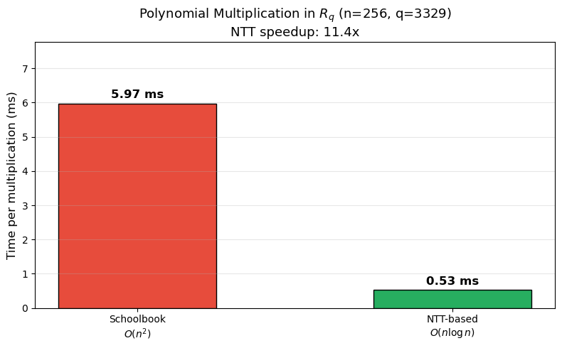
Schoolbook: 5.97 ms (mean of 20 trials)
NTT-based:  0.53 ms (mean of 20 trials)
Speedup:    11.4x
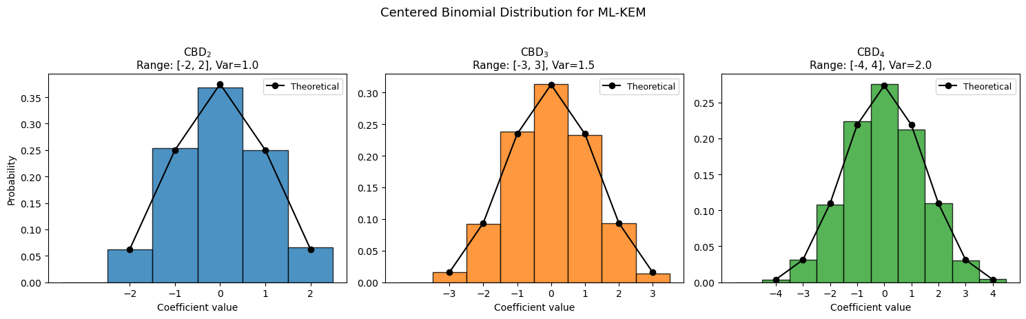
41.5 Centered Binomial Distribution#
Sampling
ML-KEM samples secret and error polynomials from the centered binomial distribution \(\text{CBD}_\eta\). For each coefficient:
This gives \(c \in \{-\eta, \ldots, \eta\}\) with probability \(\Pr[c = j] = \binom{2\eta}{\eta+j} / 2^{2\eta}\).
ML-KEM-512 uses \(\eta_1 = 3, \eta_2 = 2\).
ML-KEM-768 uses \(\eta_1 = 2, \eta_2 = 2\).
ML-KEM-1024 uses \(\eta_1 = 2, \eta_2 = 2\).
Show code cell source
import numpy as np
import matplotlib.pyplot as plt
import math

def sample_cbd(eta, num_coeffs=256, rng=None):
    """Sample polynomial coefficients from CBD_eta."""
    if rng is None:
        rng = np.random.default_rng()
    bits = rng.integers(0, 2, size=(num_coeffs, 2 * eta))
    a_sum = bits[:, :eta].sum(axis=1)
    b_sum = bits[:, eta:].sum(axis=1)
    return (a_sum - b_sum).tolist()

def cbd_from_bytes(input_bytes, eta, q=3329):
    """Sample CBD_eta from a byte array (deterministic, as in FIPS 203).
    Expects exactly 64*eta bytes.  Returns 256 coefficients mod q."""
    if len(input_bytes) != 64 * eta:
        raise ValueError(f'Need {64*eta} bytes, got {len(input_bytes)}')
    b_int = int.from_bytes(input_bytes, 'little')
    coeffs = []
    mask = (1 << eta) - 1
    for _ in range(256):
        x = b_int & ((1 << (2 * eta)) - 1)
        a = bin(x & mask).count('1')
        b = bin((x >> eta) & mask).count('1')
        coeffs.append((a - b) % q)
        b_int >>= (2 * eta)
    return coeffs

# --- Visualise the CBD for different eta values ---
rng = np.random.default_rng(42)
n_samples = 10000

fig, axes = plt.subplots(1, 3, figsize=(15, 4.5))

for idx, eta in enumerate([2, 3, 4]):
    samples = []
    for _ in range(n_samples // 256 + 1):
        samples.extend(sample_cbd(eta, 256, rng))
    samples = np.array(samples[:n_samples])

    ax = axes[idx]
    bins = np.arange(-eta - 1, eta + 2) - 0.5
    ax.hist(samples, bins=bins, density=True,
            color=f'C{idx}', edgecolor='black', alpha=0.8)

    # Overlay theoretical PMF
    x_vals = np.arange(-eta, eta + 1)
    pmf = [math.comb(2 * eta, eta + j) / (2 ** (2 * eta)) for j in x_vals]
    ax.plot(x_vals, pmf, 'ko-', markersize=6, linewidth=1.5, label='Theoretical')

    ax.set_xlabel('Coefficient value', fontsize=10)
    ax.set_ylabel('Probability' if idx == 0 else '', fontsize=10)
    ax.set_title(f'$\\mathrm{{CBD}}_{{{eta}}}$\n'
                 f'Range: [{-eta}, {eta}], Var={float(eta/2):.1f}', fontsize=11)
    ax.legend(fontsize=9)
    ax.set_xticks(range(-eta, eta + 1))

fig.suptitle('Centered Binomial Distribution for ML-KEM', fontsize=13, y=1.02)
plt.tight_layout()
plt.savefig('cbd_distributions.png', dpi=150, bbox_inches='tight')
plt.show()
41.6 Polynomial Arithmetic Helpers#
Before building the full ML-KEM, we need helper functions for polynomial addition, subtraction, and matrix-vector multiplication over \(R_q\).
import numpy as np

def poly_add(a, b, q=3329):
    """Add two polynomials in R_q (coefficient-wise mod q)."""
    return [(ai + bi) % q for ai, bi in zip(a, b)]

def poly_sub(a, b, q=3329):
    """Subtract two polynomials in R_q."""
    return [(ai - bi) % q for ai, bi in zip(a, b)]

def mat_vec_mul_ntt(A_hat, s_hat, ntt_obj):
    """Multiply matrix A_hat by vector s_hat in NTT domain."""
    k = len(A_hat)
    result = []
    for i in range(k):
        acc = [0] * 256
        for j in range(k):
            prod = ntt_obj.pointwise_multiply(A_hat[i][j], s_hat[j])
            acc = poly_add(acc, prod)
        result.append(acc)
    return result

def vec_dot_ntt(a_hat, b_hat, ntt_obj):
    """Inner product of two vectors in NTT domain."""
    k = len(a_hat)
    acc = [0] * 256
    for i in range(k):
        prod = ntt_obj.pointwise_multiply(a_hat[i], b_hat[i])
        acc = poly_add(acc, prod)
    return acc

# Quick test
ntt = NTT()
a = [1] + [0] * 255   # polynomial '1'
b = [0, 1] + [0] * 254  # polynomial 'x'

a_hat = ntt.forward(a)
b_hat = ntt.forward(b)
c_hat = ntt.pointwise_multiply(a_hat, b_hat)
c = ntt.inverse(c_hat)

# 1 * x = x, so result should be [0, 1, 0, 0, ...]
print('Product of 1 and x:')
print(f'  Result[0:5] = {c[:5]}  (expected [0, 1, 0, 0, 0])')
print(f'  Correct: {c[:5] == [0, 1, 0, 0, 0]}')
Product of 1 and x:
  Result[0:5] = [0, 1, 0, 0, 0]  (expected [0, 1, 0, 0, 0])
  Correct: True
41.7 The ML-KEM Protocol#
ML-KEM is a Key Encapsulation Mechanism (KEM) consisting of three algorithms:
KeyGen() \(\to\) \((ek, dk)\): Generate an encapsulation key and decapsulation key.
Encaps(ek) \(\to\) \((K, c)\): Produce a shared secret \(K\) and ciphertext \(c\).
Decaps(dk, c) \(\to\) \(K\): Recover the shared secret from the ciphertext.
Internal K-PKE (Public Key Encryption)#
Internally, ML-KEM wraps an IND-CPA secure public-key encryption scheme called K-PKE with the Fujisaki-Okamoto (FO) transform to achieve IND-CCA2 security.
K-PKE.KeyGen():
Sample random seed \(d\).
Derive matrix \(\hat{\mathbf{A}}\) from seed \(\rho\) (via XOF).
Sample secret \(\mathbf{s}\) and error \(\mathbf{e}\) from \(\text{CBD}_{\eta_1}\).
Compute \(\hat{\mathbf{t}} = \hat{\mathbf{A}} \cdot \hat{\mathbf{s}} + \hat{\mathbf{e}}\) (in NTT domain).
Public key: \((\hat{\mathbf{t}}, \rho)\). Secret key: \(\hat{\mathbf{s}}\).
K-PKE.Encrypt(pk, m, r):
Parse \(pk = (\hat{\mathbf{t}}, \rho)\). Derive \(\hat{\mathbf{A}}\) from \(\rho\).
Sample \(\mathbf{y}\) from \(\text{CBD}_{\eta_1}\) and \(\mathbf{e}_1, e_2\) from \(\text{CBD}_{\eta_2}\).
Compute \(\mathbf{u} = \text{NTT}^{-1}(\hat{\mathbf{A}}^T \cdot \hat{\mathbf{y}}) + \mathbf{e}_1\).
Compute \(v = \text{NTT}^{-1}(\hat{\mathbf{t}}^T \cdot \hat{\mathbf{y}}) + e_2 + \lceil q/2 \rfloor \cdot m\).
Ciphertext: \((\mathbf{u}, v)\) after compression.
Why does decryption work?
The key insight is that \(v - \mathbf{s}^T \mathbf{u} = \mathbf{e}^T \mathbf{y} - \mathbf{s}^T \mathbf{e}_1 + e_2 + \lceil q/2 \rfloor m\).
The error term \(\mathbf{e}^T \mathbf{y} - \mathbf{s}^T \mathbf{e}_1 + e_2\) is small (all vectors have small coefficients), so rounding recovers \(m\).
import numpy as np
import math

def compress(x, d, q=3329):
    """Compress: Z_q -> Z_{2^d}. Round (2^d / q) * x."""
    if isinstance(x, (list, np.ndarray)):
        return [compress(xi, d, q) for xi in x]
    return int(math.floor(((1 << d) / q) * int(x) + 0.5)) % (1 << d)

def decompress(y, d, q=3329):
    """Decompress: Z_{2^d} -> Z_q. Round (q / 2^d) * y."""
    if isinstance(y, (list, np.ndarray)):
        return [decompress(yi, d, q) for yi in y]
    return int(math.floor((q / (1 << d)) * int(y) + 0.5))

# Verify compress/decompress is lossy but close
q = 3329
for d in [1, 4, 10]:
    errors = []
    for x in range(q):
        y = compress(x, d, q)
        x_rec = decompress(y, d, q)
        err = abs(x - x_rec)
        if err > q // 2:
            err = q - err
        errors.append(err)
    print(f'd={int(d):2d}: max error = {int(max(errors)):4d}, '
          f'mean error = {float(np.mean(errors)):.1f}, '
          f'compression ratio = {float(12/d):.1f}x')
d= 1: max error =  832, mean error = 416.1, compression ratio = 12.0x
d= 4: max error =  104, mean error = 52.0, compression ratio = 3.0x
d=10: max error =    2, mean error = 0.8, compression ratio = 1.2x
41.8 Simplified ML-KEM Implementation#
We now implement a simplified ML-KEM class. For pedagogical clarity, we:
Use NumPy’s random generator instead of SHAKE-128/256 for matrix and noise generation.
Skip byte encoding/decoding (work directly with integer coefficient arrays).
Implement the core mathematical operations faithfully.
Simplification
A production ML-KEM must derive the matrix \(\mathbf{A}\) and noise vectors
deterministically from seeds using SHAKE-128/256 (XOF/PRF). Our simplified
version uses numpy.random for sampling, which preserves the mathematical
structure but not the byte-level compatibility with FIPS 203.
import numpy as np
import math

class MLKEM:
    """Simplified ML-KEM (Kyber) implementation.

    Implements the core mathematical operations of ML-KEM for
    educational purposes.  Uses numpy.random for sampling instead
    of SHAKE XOF for simplicity."""

    PARAMS = {
        'ML-KEM-512':  {'k': 2, 'eta1': 3, 'eta2': 2, 'du': 10, 'dv': 4},
        'ML-KEM-768':  {'k': 3, 'eta1': 2, 'eta2': 2, 'du': 10, 'dv': 4},
        'ML-KEM-1024': {'k': 4, 'eta1': 2, 'eta2': 2, 'du': 11, 'dv': 5},
    }

    def __init__(self, variant='ML-KEM-512', seed=None):
        self.q = 3329
        self.n = 256
        params = self.PARAMS[variant]
        self.k = params['k']
        self.eta1 = params['eta1']
        self.eta2 = params['eta2']
        self.du = params['du']
        self.dv = params['dv']
        self.variant = variant
        self.ntt = NTT(zeta=17, q=self.q)
        self.rng = np.random.default_rng(seed)

    def _sample_cbd(self, eta):
        """Sample a polynomial from CBD_eta."""
        bits = self.rng.integers(0, 2, size=(self.n, 2 * eta))
        a_sum = bits[:, :eta].sum(axis=1)
        b_sum = bits[:, eta:].sum(axis=1)
        return [(int(a) - int(b)) % self.q for a, b in zip(a_sum, b_sum)]

    def _sample_uniform(self):
        """Sample a uniformly random polynomial in R_q."""
        return [int(x) for x in self.rng.integers(0, self.q, size=self.n)]

    def _compress(self, x, d):
        return compress(x, d, self.q)

    def _decompress(self, y, d):
        return decompress(y, d, self.q)

    def keygen(self):
        """Generate ML-KEM key pair.  Returns (ek, dk)."""
        k = self.k
        # In ML-KEM, matrix A is generated directly in NTT domain
        A_hat = [[self._sample_uniform() for _ in range(k)] for _ in range(k)]
        s = [self._sample_cbd(self.eta1) for _ in range(k)]
        s_hat = self.ntt.ntt_vector(s)
        e = [self._sample_cbd(self.eta1) for _ in range(k)]
        e_hat = self.ntt.ntt_vector(e)
        As_hat = mat_vec_mul_ntt(A_hat, s_hat, self.ntt)
        t_hat = [poly_add(As_hat[i], e_hat[i]) for i in range(k)]
        ek = (A_hat, t_hat)
        dk = (s_hat, ek)
        return ek, dk

    def encaps(self, ek):
        """Encapsulate: produce shared secret and ciphertext."""
        A_hat, t_hat = ek
        k = self.k
        m = [int(x) for x in self.rng.integers(0, 2, size=self.n)]
        y = [self._sample_cbd(self.eta1) for _ in range(k)]
        y_hat = self.ntt.ntt_vector(y)
        e1 = [self._sample_cbd(self.eta2) for _ in range(k)]
        e2 = self._sample_cbd(self.eta2)
        A_hat_T = [[A_hat[j][i] for j in range(k)] for i in range(k)]
        Ay_hat = mat_vec_mul_ntt(A_hat_T, y_hat, self.ntt)
        Ay = self.ntt.intt_vector(Ay_hat)
        u = [poly_add(Ay[i], e1[i]) for i in range(k)]
        ty_hat = vec_dot_ntt(t_hat, y_hat, self.ntt)
        ty = self.ntt.inverse(ty_hat)
        q_half = (self.q + 1) // 2
        m_scaled = [(mi * q_half) % self.q for mi in m]
        v = poly_add(poly_add(ty, e2), m_scaled)
        u_comp = [self._compress(ui, self.du) for ui in u]
        v_comp = self._compress(v, self.dv)
        ciphertext = (u_comp, v_comp)
        shared_secret = m
        return shared_secret, ciphertext

    def decaps(self, dk, ciphertext):
        """Decapsulate: recover shared secret from ciphertext."""
        s_hat, ek = dk
        u_comp, v_comp = ciphertext
        k = self.k
        u = [self._decompress(ui, self.du) for ui in u_comp]
        v = self._decompress(v_comp, self.dv)
        u_hat = self.ntt.ntt_vector(u)
        su_hat = vec_dot_ntt(s_hat, u_hat, self.ntt)
        su = self.ntt.inverse(su_hat)
        w = poly_sub(v, su)
        m_recovered = self._compress(w, 1)
        return m_recovered

print('MLKEM class defined with variants:', list(MLKEM.PARAMS.keys()))
MLKEM class defined with variants: ['ML-KEM-512', 'ML-KEM-768', 'ML-KEM-1024']
Pedagogical Simplification
This implementation demonstrates the core mathematical structure of ML-KEM but omits several components required by FIPS 203: the Fujisaki-Okamoto transform, the shared-secret KDF (SHA3-256), seed-derived matrix generation (XOF), byte encoding/decoding, and KAT compatibility. It should not be used for any security-sensitive application.
41.9 Full Key Exchange Demonstration#
Let us run the complete ML-KEM key exchange protocol: Alice generates a key pair, Bob encapsulates a shared secret, and Alice decapsulates to recover it.
Shared secret in FIPS 203
In this simplified demo, the “shared secret” is the raw 256-bit message vector. The actual FIPS 203 standard derives a 32-byte shared secret by applying a KDF (SHA3-256) as part of the Fujisaki-Okamoto transform. Our implementation omits the FO transform and returns the plaintext message directly.
import numpy as np

print('=' * 65)
print('         ML-KEM Key Exchange Demonstration')
print('=' * 65)

for variant in ['ML-KEM-512', 'ML-KEM-768', 'ML-KEM-1024']:
    kem = MLKEM(variant=variant, seed=2024)
    ek, dk = kem.keygen()
    K_bob, ciphertext = kem.encaps(ek)
    K_alice = kem.decaps(dk, ciphertext)
    match = (K_bob == K_alice)
    n_bits = sum(1 for a, b in zip(K_bob, K_alice) if a == b)

    print(f'\n--- {variant} (k={kem.k}) ---')
    print(f'  Shared secret length: {len(K_bob)} bits')
    print(f'  Bob   K[0:16]: {K_bob[:16]}')
    print(f'  Alice K[0:16]: {K_alice[:16]}')
    print(f'  Matching bits: {n_bits} / {len(K_bob)}')
    print(f'  Keys match:    {match}')

print('\n' + '=' * 65)
=================================================================
         ML-KEM Key Exchange Demonstration
=================================================================

--- ML-KEM-512 (k=2) ---
  Shared secret length: 256 bits
  Bob   K[0:16]: [0, 0, 0, 1, 1, 1, 1, 0, 1, 0, 1, 0, 0, 1, 0, 0]
  Alice K[0:16]: [0, 0, 0, 1, 1, 1, 1, 0, 1, 0, 1, 0, 0, 1, 0, 0]
  Matching bits: 256 / 256
  Keys match:    True

--- ML-KEM-768 (k=3) ---
  Shared secret length: 256 bits
  Bob   K[0:16]: [0, 0, 0, 0, 0, 0, 1, 0, 0, 1, 1, 1, 1, 0, 1, 1]
  Alice K[0:16]: [0, 0, 0, 0, 0, 0, 1, 0, 0, 1, 1, 1, 1, 0, 1, 1]
  Matching bits: 256 / 256
  Keys match:    True

--- ML-KEM-1024 (k=4) ---
  Shared secret length: 256 bits
  Bob   K[0:16]: [1, 1, 0, 0, 0, 0, 1, 0, 0, 0, 0, 1, 1, 0, 1, 1]
  Alice K[0:16]: [1, 1, 0, 0, 0, 0, 1, 0, 0, 0, 0, 1, 1, 0, 1, 1]
  Matching bits: 256 / 256
  Keys match:    True

=================================================================
Decryption Noise Analysis#
The correctness of ML-KEM depends on the decryption noise being small enough that rounding recovers the message. Let us measure the actual noise distribution.
Show code cell source
import numpy as np
import matplotlib.pyplot as plt

def measure_decryption_noise(variant='ML-KEM-512', seed=42):
    """Measure decryption noise (without compression) for one exchange."""
    kem = MLKEM(variant=variant, seed=seed)
    k = kem.k
    q = kem.q
    ntt_obj = kem.ntt
    A_hat = [[kem._sample_uniform() for _ in range(k)] for _ in range(k)]
    s = [kem._sample_cbd(kem.eta1) for _ in range(k)]
    s_hat = ntt_obj.ntt_vector(s)
    e = [kem._sample_cbd(kem.eta1) for _ in range(k)]
    e_hat = ntt_obj.ntt_vector(e)
    As_hat = mat_vec_mul_ntt(A_hat, s_hat, ntt_obj)
    t_hat = [poly_add(As_hat[i], e_hat[i]) for i in range(k)]
    m = [int(x) for x in kem.rng.integers(0, 2, size=256)]
    y = [kem._sample_cbd(kem.eta1) for _ in range(k)]
    y_hat = ntt_obj.ntt_vector(y)
    e1 = [kem._sample_cbd(kem.eta2) for _ in range(k)]
    e2 = kem._sample_cbd(kem.eta2)
    A_hat_T = [[A_hat[j][i] for j in range(k)] for i in range(k)]
    Ay_hat = mat_vec_mul_ntt(A_hat_T, y_hat, ntt_obj)
    Ay = ntt_obj.intt_vector(Ay_hat)
    u = [poly_add(Ay[i], e1[i]) for i in range(k)]
    ty_hat = vec_dot_ntt(t_hat, y_hat, ntt_obj)
    ty = ntt_obj.inverse(ty_hat)
    q_half = (q + 1) // 2
    m_scaled = [(mi * q_half) % q for mi in m]
    v = poly_add(poly_add(ty, e2), m_scaled)
    u_hat = ntt_obj.ntt_vector(u)
    su_hat = vec_dot_ntt(s_hat, u_hat, ntt_obj)
    su = ntt_obj.inverse(su_hat)
    w = poly_sub(v, su)
    noise = []
    for wi, mi in zip(w, m_scaled):
        diff = (wi - mi) % q
        if diff > q // 2:
            diff -= q
        noise.append(diff)
    return noise, m

fig, axes = plt.subplots(1, 3, figsize=(16, 4.5))
variants = ['ML-KEM-512', 'ML-KEM-768', 'ML-KEM-1024']
colors = ['#3498db', '#e67e22', '#2ecc71']

for idx, (variant, color) in enumerate(zip(variants, colors)):
    all_noise = []
    for trial_seed in range(50):
        noise, _ = measure_decryption_noise(variant, seed=trial_seed)
        all_noise.extend(noise)
    all_noise = np.array(all_noise)
    ax = axes[idx]
    ax.hist(all_noise, bins=80, color=color, edgecolor='black',
            alpha=0.8, density=True)
    ax.axvline(x=0, color='red', linestyle='--', linewidth=1)
    threshold = 3329 // 4
    ax.axvline(x=-threshold, color='darkred', linestyle=':', linewidth=1.5,
               label=f'Threshold (+/-{threshold})')
    ax.axvline(x=threshold, color='darkred', linestyle=':', linewidth=1.5)
    ax.set_xlabel('Noise value', fontsize=10)
    ax.set_ylabel('Density' if idx == 0 else '', fontsize=10)
    ax.set_title(f'{variant} (k={MLKEM.PARAMS[variant]["k"]})\n'
                 f'std={float(all_noise.std()):.1f}, max|noise|={np.max(np.abs(all_noise))}',
                 fontsize=11)
    ax.legend(fontsize=8)

fig.suptitle('ML-KEM Decryption Noise Distribution (no compression)', fontsize=13, y=1.02)
plt.tight_layout()
plt.savefig('mlkem_noise_distribution.png', dpi=150, bbox_inches='tight')
plt.show()

print('If |noise| < q/4 = 832 for all coefficients, decryption succeeds.')
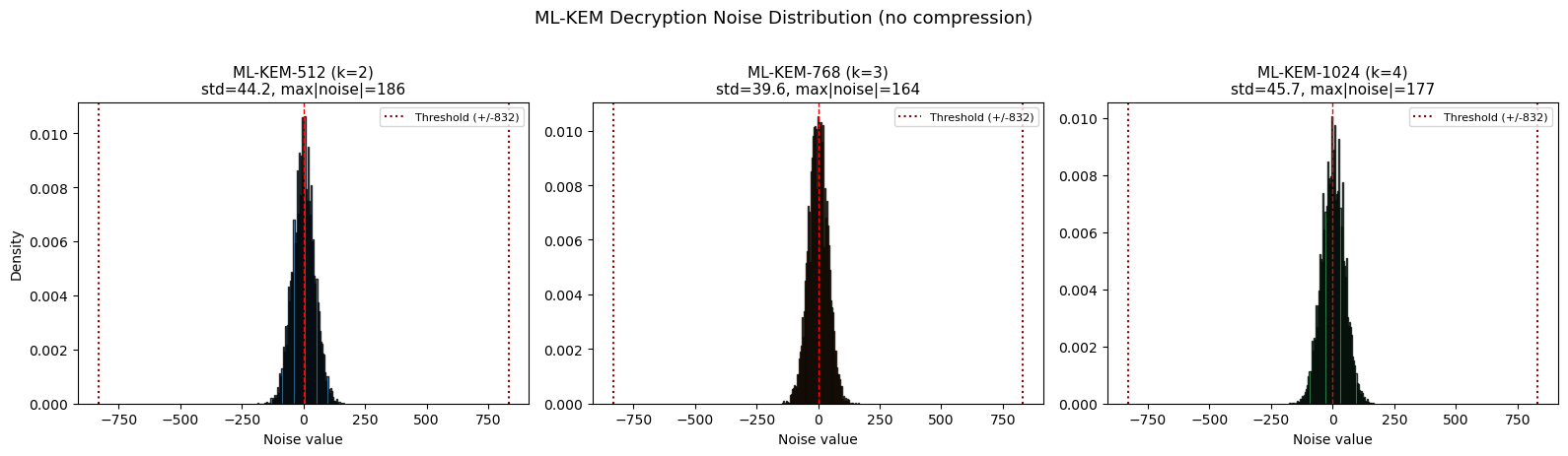
If |noise| < q/4 = 832 for all coefficients, decryption succeeds.
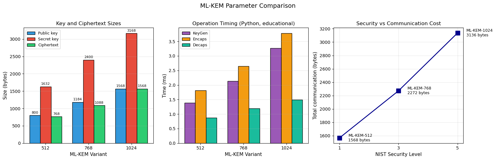
41.10 Parameter Comparison: ML-KEM-512/768/1024#
Parameter |
ML-KEM-512 |
ML-KEM-768 |
ML-KEM-1024 |
|---|---|---|---|
\(k\) (module rank) |
2 |
3 |
4 |
\(q\) (modulus) |
3329 |
3329 |
3329 |
\(\eta_1\) |
3 |
2 |
2 |
\(\eta_2\) |
2 |
2 |
2 |
\((d_u, d_v)\) |
(10, 4) |
(10, 4) |
(11, 5) |
Public key (bytes) |
800 |
1184 |
1568 |
Secret key (bytes) |
1632 |
2400 |
3168 |
Ciphertext (bytes) |
768 |
1088 |
1568 |
Shared secret (bytes) |
32 |
32 |
32 |
NIST security level |
1 |
3 |
5 |
Show code cell source
import numpy as np
import matplotlib.pyplot as plt
import time

variants = ['ML-KEM-512', 'ML-KEM-768', 'ML-KEM-1024']
pk_sizes = [800, 1184, 1568]
sk_sizes = [1632, 2400, 3168]
ct_sizes = [768, 1088, 1568]
nist_levels = [1, 3, 5]

fig, axes = plt.subplots(1, 3, figsize=(16, 5))

# Plot 1: Key and ciphertext sizes
x = np.arange(len(variants))
w = 0.25
bars1 = axes[0].bar(x - w, pk_sizes, w, label='Public key', color='#3498db',
                     edgecolor='black')
bars2 = axes[0].bar(x, sk_sizes, w, label='Secret key', color='#e74c3c',
                     edgecolor='black')
bars3 = axes[0].bar(x + w, ct_sizes, w, label='Ciphertext', color='#2ecc71',
                     edgecolor='black')
axes[0].set_xticks(x)
axes[0].set_xticklabels(['512', '768', '1024'])
axes[0].set_xlabel('ML-KEM Variant', fontsize=11)
axes[0].set_ylabel('Size (bytes)', fontsize=11)
axes[0].set_title('Key and Ciphertext Sizes', fontsize=12)
axes[0].legend(fontsize=9)
axes[0].grid(axis='y', alpha=0.3)
for bars in [bars1, bars2, bars3]:
    for bar in bars:
        h = bar.get_height()
        axes[0].text(bar.get_x() + bar.get_width()/2, h + 30,
                     f'{int(h)}', ha='center', va='bottom', fontsize=8)

# Plot 2: Timing comparison
keygen_times = []
encaps_times = []
decaps_times = []
for variant in variants:
    kg_t, en_t, de_t = [], [], []
    for trial in range(5):
        kem = MLKEM(variant=variant, seed=trial)
        t0 = time.perf_counter()
        ek, dk = kem.keygen()
        t1 = time.perf_counter()
        kg_t.append(t1 - t0)
        t0 = time.perf_counter()
        K, ct = kem.encaps(ek)
        t1 = time.perf_counter()
        en_t.append(t1 - t0)
        t0 = time.perf_counter()
        K2 = kem.decaps(dk, ct)
        t1 = time.perf_counter()
        de_t.append(t1 - t0)
    keygen_times.append(np.mean(kg_t) * 1000)
    encaps_times.append(np.mean(en_t) * 1000)
    decaps_times.append(np.mean(de_t) * 1000)

bars1 = axes[1].bar(x - w, keygen_times, w, label='KeyGen', color='#9b59b6',
                     edgecolor='black')
bars2 = axes[1].bar(x, encaps_times, w, label='Encaps', color='#f39c12',
                     edgecolor='black')
bars3 = axes[1].bar(x + w, decaps_times, w, label='Decaps', color='#1abc9c',
                     edgecolor='black')
axes[1].set_xticks(x)
axes[1].set_xticklabels(['512', '768', '1024'])
axes[1].set_xlabel('ML-KEM Variant', fontsize=11)
axes[1].set_ylabel('Time (ms)', fontsize=11)
axes[1].set_title('Operation Timing (Python, educational)', fontsize=12)
axes[1].legend(fontsize=9)
axes[1].grid(axis='y', alpha=0.3)

# Plot 3: Security level vs total communication
total_comm = [pk + ct for pk, ct in zip(pk_sizes, ct_sizes)]
axes[2].plot(nist_levels, total_comm, 's-', color='darkblue', linewidth=2,
             markersize=10)
for i, (nl, tc, var) in enumerate(zip(nist_levels, total_comm, variants)):
    axes[2].annotate(f'{var}\n{tc} bytes', xy=(nl, tc),
                     xytext=(nl + 0.3, tc), fontsize=9, va='center')
axes[2].set_xlabel('NIST Security Level', fontsize=11)
axes[2].set_ylabel('Total communication (bytes)', fontsize=11)
axes[2].set_title('Security vs Communication Cost', fontsize=12)
axes[2].set_xticks([1, 3, 5])
axes[2].grid(True, alpha=0.3)

fig.suptitle('ML-KEM Parameter Comparison', fontsize=14, y=1.02)
plt.tight_layout()
plt.savefig('mlkem_parameter_comparison.png', dpi=150, bbox_inches='tight')
plt.show()
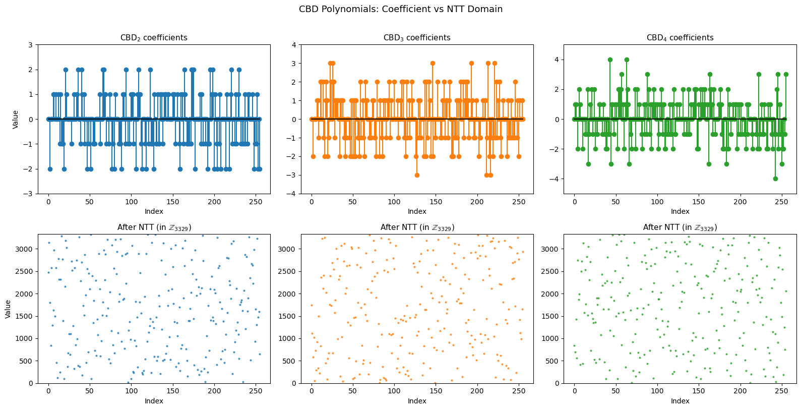
41.11 Visualising the NTT#
NTT Spectrum of Secret Polynomials#
The NTT transforms small-coefficient polynomials (from CBD) into the frequency domain. Let us visualise what CBD samples look like before and after NTT.
Show code cell source
import numpy as np
import matplotlib.pyplot as plt

ntt = NTT()
rng = np.random.default_rng(42)

fig, axes = plt.subplots(2, 3, figsize=(16, 8))

for col, eta in enumerate([2, 3, 4]):
    bits = rng.integers(0, 2, size=(256, 2 * eta))
    a_sum = bits[:, :eta].sum(axis=1)
    b_sum = bits[:, eta:].sum(axis=1)
    poly = [(int(a) - int(b)) % 3329 for a, b in zip(a_sum, b_sum)]
    poly_centered = [c if c <= 3329 // 2 else c - 3329 for c in poly]
    poly_ntt = ntt.forward(poly)

    axes[0, col].stem(range(256), poly_centered, linefmt=f'C{col}-',
                       markerfmt=f'C{col}o', basefmt='k-')
    axes[0, col].set_title(f'$\\mathrm{{CBD}}_{{{eta}}}$ coefficients', fontsize=11)
    axes[0, col].set_xlabel('Index', fontsize=10)
    axes[0, col].set_ylabel('Value' if col == 0 else '', fontsize=10)
    axes[0, col].set_ylim(-eta - 1, eta + 1)

    axes[1, col].scatter(range(256), poly_ntt, s=4, c=f'C{col}', alpha=0.7)
    axes[1, col].set_title(f'After NTT (in $\\mathbb{{Z}}_{{3329}}$)', fontsize=11)
    axes[1, col].set_xlabel('Index', fontsize=10)
    axes[1, col].set_ylabel('Value' if col == 0 else '', fontsize=10)
    axes[1, col].set_ylim(0, 3329)

fig.suptitle('CBD Polynomials: Coefficient vs NTT Domain', fontsize=13, y=1.01)
plt.tight_layout()
plt.savefig('ntt_spectrum_cbd.png', dpi=150, bbox_inches='tight')
plt.show()
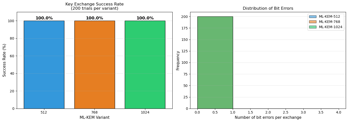
41.12 Decryption Failure Probability#
ML-KEM has a non-zero but negligible decryption failure probability. A failure occurs when the decryption noise exceeds \(\lfloor q/4 \rfloor = 832\) for some coefficient. The failure probability is designed to be \(< 2^{-139}\) for ML-KEM-512.
Let us empirically estimate the failure rate by running many key exchanges.
Show code cell source
import numpy as np
import matplotlib.pyplot as plt

n_trials = 200
variants = ['ML-KEM-512', 'ML-KEM-768', 'ML-KEM-1024']
results = {}

for variant in variants:
    successes = 0
    bit_errors_list = []
    for trial in range(n_trials):
        kem = MLKEM(variant=variant, seed=trial * 1000 + 7)
        ek, dk = kem.keygen()
        K_send, ct = kem.encaps(ek)
        K_recv = kem.decaps(dk, ct)
        n_correct = sum(1 for a, b in zip(K_send, K_recv) if a == b)
        bit_errors_list.append(256 - n_correct)
        if K_send == K_recv:
            successes += 1
    results[variant] = {'success_rate': successes / n_trials,
                        'bit_errors': bit_errors_list}
    print(f'{variant}: {successes}/{n_trials} successful '
          f'({float(100*successes/n_trials):.1f}%)')

fig, axes = plt.subplots(1, 2, figsize=(14, 5))

# Success rates
variant_names = ['512', '768', '1024']
rates = [results[v]['success_rate'] * 100 for v in variants]
colors = ['#3498db', '#e67e22', '#2ecc71']
bars = axes[0].bar(variant_names, rates, color=colors, edgecolor='black')
for bar, rate in zip(bars, rates):
    axes[0].text(bar.get_x() + bar.get_width()/2, bar.get_height() + 0.5,
                 f'{float(rate):.1f}%', ha='center', va='bottom', fontsize=12,
                 fontweight='bold')
axes[0].set_xlabel('ML-KEM Variant', fontsize=11)
axes[0].set_ylabel('Success Rate (%)', fontsize=11)
axes[0].set_title(f'Key Exchange Success Rate\n({n_trials} trials per variant)',
                  fontsize=12)
axes[0].set_ylim(0, 110)
axes[0].grid(axis='y', alpha=0.3)

# Bit error distribution
for i, (variant, color) in enumerate(zip(variants, colors)):
    errs = results[variant]['bit_errors']
    axes[1].hist(errs, bins=range(0, max(max(errs) + 2, 5)),
                 alpha=0.6, color=color, edgecolor='black', label=f'{variant}')
axes[1].set_xlabel('Number of bit errors per exchange', fontsize=11)
axes[1].set_ylabel('Frequency', fontsize=11)
axes[1].set_title('Distribution of Bit Errors', fontsize=12)
axes[1].legend(fontsize=10)
axes[1].grid(axis='y', alpha=0.3)

plt.tight_layout()
plt.savefig('mlkem_success_rate.png', dpi=150, bbox_inches='tight')
plt.show()
ML-KEM-512: 200/200 successful (100.0%)
ML-KEM-768: 200/200 successful (100.0%)
ML-KEM-1024: 200/200 successful (100.0%)
41.13 Visualising Twiddle Factors#
The NTT twiddle factors \(\zeta^{\text{br}(i)}\) for \(i = 0, \ldots, 127\) form a specific pattern in \(\mathbb{Z}_q\). Let us visualise their structure.
Show code cell source
import numpy as np
import matplotlib.pyplot as plt

ntt = NTT()
zetas = ntt.ntt_zetas

fig, axes = plt.subplots(1, 2, figsize=(14, 5))

axes[0].scatter(range(128), zetas, c=range(128), cmap='viridis',
                s=25, edgecolors='black', linewidths=0.5)
axes[0].set_xlabel('Index $i$', fontsize=11)
axes[0].set_ylabel('$\\zeta^{\\mathrm{br}(i)}$ mod $q$', fontsize=11)
axes[0].set_title('NTT Twiddle Factors ($q = 3329$, $\\zeta = 17$)', fontsize=12)
axes[0].grid(True, alpha=0.3)

# Map Z_q values to angles on unit circle analogy
angles = [2 * np.pi * z / 3329 for z in zetas]
axes[1].scatter([np.cos(a) for a in angles],
                [np.sin(a) for a in angles],
                c=range(128), cmap='plasma', s=30,
                edgecolors='black', linewidths=0.5)
circle = np.linspace(0, 2 * np.pi, 200)
axes[1].plot(np.cos(circle), np.sin(circle), 'k-', alpha=0.2)
axes[1].set_xlabel('$\\cos(2\\pi \\zeta / q)$', fontsize=11)
axes[1].set_ylabel('$\\sin(2\\pi \\zeta / q)$', fontsize=11)
axes[1].set_title('Twiddle Factors Mapped to Unit Circle', fontsize=12)
axes[1].set_aspect('equal')
axes[1].grid(True, alpha=0.3)

plt.tight_layout()
plt.savefig('ntt_twiddle_factors.png', dpi=150, bbox_inches='tight')
plt.show()

print(f'First 10 twiddle factors: {zetas[:10]}')
print(f'zeta[0] = {zetas[0]}  (should be 17^0 = 1)')
print(f'zeta[1] = {zetas[1]}  (should be 17^64 mod 3329 = {pow(17,64,3329)})')
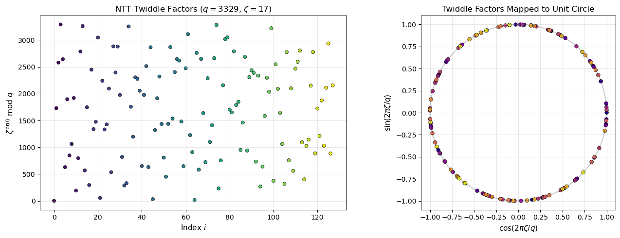
First 10 twiddle factors: [1, 1729, 2580, 3289, 2642, 630, 1897, 848, 1062, 1919]
zeta[0] = 1  (should be 17^0 = 1)
zeta[1] = 1729  (should be 17^64 mod 3329 = 1729)
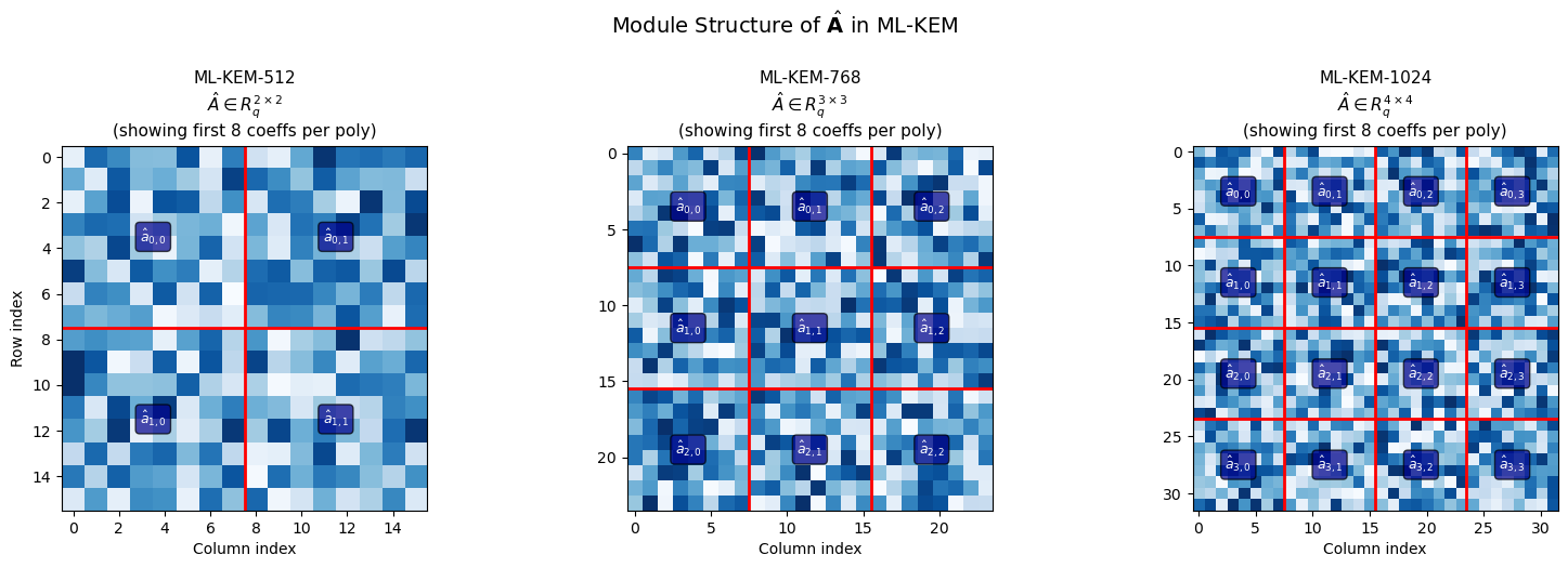
41.14 The Module Structure of ML-KEM#
The “Module” in Module-LWE refers to working with vectors and matrices over \(R_q\) rather than individual ring elements. This provides a flexible way to scale security by adjusting the module rank \(k\).
Ring-LWE vs Module-LWE vs LWE
LWE (Regev, 2005): vectors over \(\mathbb{Z}_q\). Large keys.
Ring-LWE (Lyubashevsky-Peikert-Regev, 2010): single elements of \(R_q\). Compact keys but security relies on ring structure.
Module-LWE (Langlois-Stehle, 2015): vectors of \(R_q\) elements. Intermediate key sizes with tuneable security via \(k\). ML-KEM uses this approach.
Show code cell source
import numpy as np
import matplotlib.pyplot as plt

fig, axes = plt.subplots(1, 3, figsize=(16, 5))
rng = np.random.default_rng(42)

for idx, (k, variant) in enumerate([(2, '512'), (3, '768'), (4, '1024')]):
    A = rng.integers(0, 3329, size=(k * 8, k * 8))
    ax = axes[idx]
    im = ax.imshow(A, cmap='Blues', aspect='equal')
    for i in range(1, k):
        ax.axhline(y=i * 8 - 0.5, color='red', linewidth=2)
        ax.axvline(x=i * 8 - 0.5, color='red', linewidth=2)
    ax.set_title(f'ML-KEM-{variant}\n$\\hat{{A}} \\in R_q^{{{k} \\times {k}}}$\n'
                 f'(showing first 8 coeffs per poly)', fontsize=11)
    ax.set_xlabel('Column index', fontsize=10)
    ax.set_ylabel('Row index' if idx == 0 else '', fontsize=10)
    for bi in range(k):
        for bj in range(k):
            ax.text(bj * 8 + 3.5, bi * 8 + 3.5,
                    f'$\\hat{{a}}_{{{bi},{bj}}}$',
                    ha='center', va='center', fontsize=9,
                    color='white', fontweight='bold',
                    bbox=dict(boxstyle='round', facecolor='darkblue', alpha=0.7))

fig.suptitle('Module Structure of $\\hat{\\mathbf{A}}$ in ML-KEM', fontsize=14, y=1.02)
plt.tight_layout()
plt.savefig('mlkem_module_structure.png', dpi=150, bbox_inches='tight')
plt.show()
41.15 Why Decryption Works: A Visual Proof#
During encryption, Bob computes:
During decryption, Alice computes:
The noise \(\mathbf{e}^T \mathbf{y} - \mathbf{s}^T \mathbf{e}_1 + e_2\) is small since all these vectors have small coefficients.
Show code cell source
import numpy as np
import matplotlib.pyplot as plt

kem = MLKEM(variant='ML-KEM-512', seed=77)
q = kem.q
k = kem.k
ntt_obj = kem.ntt

# KeyGen
A_hat = [[kem._sample_uniform() for _ in range(k)] for _ in range(k)]
s = [kem._sample_cbd(kem.eta1) for _ in range(k)]
s_hat = ntt_obj.ntt_vector(s)
e = [kem._sample_cbd(kem.eta1) for _ in range(k)]
e_hat = ntt_obj.ntt_vector(e)
As_hat = mat_vec_mul_ntt(A_hat, s_hat, ntt_obj)
t_hat = [poly_add(As_hat[i], e_hat[i]) for i in range(k)]

# Encrypt (no compression)
m = [int(x) for x in kem.rng.integers(0, 2, size=256)]
y = [kem._sample_cbd(kem.eta1) for _ in range(k)]
y_hat = ntt_obj.ntt_vector(y)
e1 = [kem._sample_cbd(kem.eta2) for _ in range(k)]
e2 = kem._sample_cbd(kem.eta2)
A_hat_T = [[A_hat[j][i] for j in range(k)] for i in range(k)]
Ay_hat = mat_vec_mul_ntt(A_hat_T, y_hat, ntt_obj)
Ay = ntt_obj.intt_vector(Ay_hat)
u = [poly_add(Ay[i], e1[i]) for i in range(k)]
ty_hat = vec_dot_ntt(t_hat, y_hat, ntt_obj)
ty = ntt_obj.inverse(ty_hat)
q_half = (q + 1) // 2
m_scaled = [(mi * q_half) % q for mi in m]
v = poly_add(poly_add(ty, e2), m_scaled)

# Decrypt
u_hat = ntt_obj.ntt_vector(u)
su_hat = vec_dot_ntt(s_hat, u_hat, ntt_obj)
su = ntt_obj.inverse(su_hat)
w = poly_sub(v, su)

fig, axes = plt.subplots(2, 2, figsize=(14, 9))

# Plot 1: Original message (scaled)
axes[0, 0].stem(range(256), m_scaled, linefmt='b-', markerfmt='bo',
                basefmt='k-')
axes[0, 0].axhline(y=q_half, color='red', linestyle='--', alpha=0.5,
                    label=f'q/2 = {q_half}')
axes[0, 0].set_title('Encoded message $\\lceil q/2 \\rfloor \cdot  m$', fontsize=12)
axes[0, 0].set_ylabel('Value', fontsize=10)
axes[0, 0].legend(fontsize=9)

# Plot 2: Decrypted w (raw)
colors_pts = ['red' if mi == 1 else 'blue' for mi in m]
axes[0, 1].scatter(range(256), w, s=5, c=colors_pts, alpha=0.7)
axes[0, 1].axhline(y=q_half, color='green', linestyle='--', alpha=0.5)
axes[0, 1].axhline(y=q // 4, color='orange', linestyle=':', alpha=0.5)
axes[0, 1].axhline(y=3 * q // 4, color='orange', linestyle=':', alpha=0.5)
axes[0, 1].set_title('Decrypted $w = v - \\mathbf{s}^T \\mathbf{u}$\n'
                      '(red=bit 1, blue=bit 0)', fontsize=12)
axes[0, 1].set_ylabel('Value in $\\mathbb{Z}_q$', fontsize=10)

# Plot 3: Noise (w - m_scaled)
noise = [(wi - mi) % q for wi, mi in zip(w, m_scaled)]
noise_centered = [n if n <= q // 2 else n - q for n in noise]
axes[1, 0].stem(range(256), noise_centered, linefmt='r-', markerfmt='ro',
                basefmt='k-')
axes[1, 0].axhline(y=q // 4, color='darkred', linestyle=':', linewidth=1.5,
                    label=f'Threshold (+/-{q//4})')
axes[1, 0].axhline(y=-q // 4, color='darkred', linestyle=':', linewidth=1.5)
axes[1, 0].set_title('Decryption noise $w - \\lceil q/2 \\rfloor \cdot  m$', fontsize=12)
axes[1, 0].set_xlabel('Coefficient index', fontsize=10)
axes[1, 0].set_ylabel('Noise value', fontsize=10)
axes[1, 0].legend(fontsize=9)

# Plot 4: Decision regions
axes[1, 1].scatter(range(256), w, s=5, c=colors_pts, alpha=0.7)
axes[1, 1].axhspan(0, q // 4, alpha=0.1, color='blue', label='Decode as 0')
axes[1, 1].axhspan(q // 4, 3 * q // 4, alpha=0.1, color='red', label='Decode as 1')
axes[1, 1].axhspan(3 * q // 4, q, alpha=0.1, color='blue')
axes[1, 1].set_title('Decision Regions for Message Recovery', fontsize=12)
axes[1, 1].set_xlabel('Coefficient index', fontsize=10)
axes[1, 1].set_ylabel('Value in $\\mathbb{Z}_q$', fontsize=10)
axes[1, 1].legend(fontsize=9)

fig.suptitle('ML-KEM-512: Encryption, Decryption, and Noise', fontsize=14, y=1.01)
plt.tight_layout()
plt.savefig('mlkem_correctness_visual.png', dpi=150, bbox_inches='tight')
plt.show()

max_noise = max(abs(n) for n in noise_centered)
print(f'Maximum |noise| = {max_noise} (threshold = {q//4})')
print(f'Noise safely below threshold: {max_noise < q//4}')
<>:47: SyntaxWarning: invalid escape sequence '\c'
<>:69: SyntaxWarning: invalid escape sequence '\c'
<>:47: SyntaxWarning: invalid escape sequence '\c'
<>:69: SyntaxWarning: invalid escape sequence '\c'
/var/folders/z7/wp7m8p7x1250jzvklw5z24mm0000gn/T/ipykernel_72578/395299474.py:47: SyntaxWarning: invalid escape sequence '\c'
  axes[0, 0].set_title('Encoded message $\\lceil q/2 \\rfloor \cdot  m$', fontsize=12)
/var/folders/z7/wp7m8p7x1250jzvklw5z24mm0000gn/T/ipykernel_72578/395299474.py:69: SyntaxWarning: invalid escape sequence '\c'
  axes[1, 0].set_title('Decryption noise $w - \\lceil q/2 \\rfloor \cdot  m$', fontsize=12)
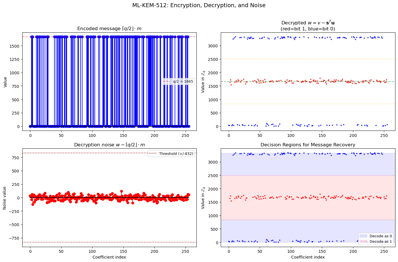
Maximum |noise| = 127 (threshold = 832)
Noise safely below threshold: True
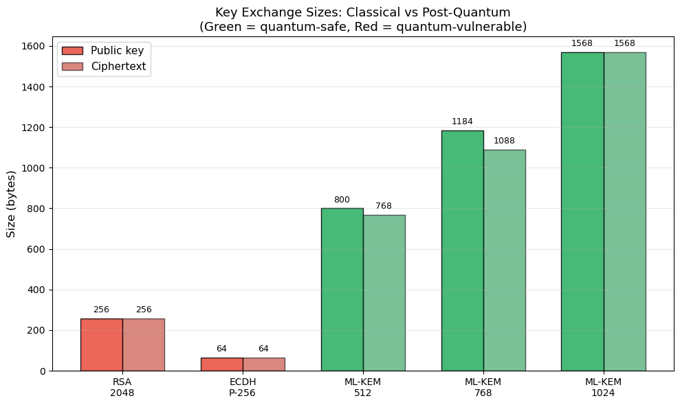
41.16 ML-KEM vs Classical Key Exchange#
Scheme |
Public Key |
Ciphertext |
Security |
Quantum Safe? |
|---|---|---|---|---|
RSA-2048 |
256 B |
256 B |
~112 bits |
No |
ECDH P-256 |
64 B |
64 B |
~128 bits |
No |
ML-KEM-512 |
800 B |
768 B |
~118 bits |
Yes |
ML-KEM-768 |
1184 B |
1088 B |
~182 bits |
Yes |
ML-KEM-1024 |
1568 B |
1568 B |
~256 bits |
Yes |
Practical impact
While ML-KEM keys are 4–20x larger than ECDH keys, they are still small enough for most applications. The computational cost is comparable to or faster than RSA. ML-KEM is already being deployed in TLS 1.3 (as a hybrid with X25519) by major browsers and cloud providers.
Show code cell source
import numpy as np
import matplotlib.pyplot as plt

schemes = ['RSA\n2048', 'ECDH\nP-256', 'ML-KEM\n512', 'ML-KEM\n768', 'ML-KEM\n1024']
pk_sizes = [256, 64, 800, 1184, 1568]
ct_sizes = [256, 64, 768, 1088, 1568]
quantum_safe = [False, False, True, True, True]

fig, ax = plt.subplots(figsize=(10, 6))
x = np.arange(len(schemes))
w = 0.35
colors_pk = ['#e74c3c' if not qs else '#27ae60' for qs in quantum_safe]
colors_ct = ['#c0392b' if not qs else '#229954' for qs in quantum_safe]

bars1 = ax.bar(x - w/2, pk_sizes, w, label='Public key', color=colors_pk,
               edgecolor='black', alpha=0.85)
bars2 = ax.bar(x + w/2, ct_sizes, w, label='Ciphertext', color=colors_ct,
               edgecolor='black', alpha=0.6)

for bar, val in zip(bars1, pk_sizes):
    ax.text(bar.get_x() + bar.get_width()/2, bar.get_height() + 20,
            f'{val}', ha='center', va='bottom', fontsize=9)
for bar, val in zip(bars2, ct_sizes):
    ax.text(bar.get_x() + bar.get_width()/2, bar.get_height() + 20,
            f'{val}', ha='center', va='bottom', fontsize=9)

ax.set_xticks(x)
ax.set_xticklabels(schemes)
ax.set_ylabel('Size (bytes)', fontsize=12)
ax.set_title('Key Exchange Sizes: Classical vs Post-Quantum\n'
             '(Green = quantum-safe, Red = quantum-vulnerable)', fontsize=13)
ax.legend(fontsize=11)
ax.grid(axis='y', alpha=0.3)

plt.tight_layout()
plt.savefig('mlkem_vs_classical_sizes.png', dpi=150, bbox_inches='tight')
plt.show()
41.17 Exercises#
Exercise 41.1: NTT Round-Trip
Verify that the NTT is its own (scaled) inverse. For a random polynomial \(f \in R_q\), compute \(\hat{f} = \text{NTT}(f)\) and \(f' = \text{NTT}^{-1}(\hat{f})\). Show that \(f' = f\) for 100 random polynomials.
Then measure: what is the maximum intermediate value that appears during NTT computation? How does this relate to the choice of \(q\)?
Hint
Modify the forward() method to track the maximum value seen at each butterfly
step. The intermediate values can exceed \(q\) before modular reduction.
Exercise 41.2: CBD Variance
Prove analytically that the variance of \(\text{CBD}_\eta\) is \(\eta/2\). Then verify experimentally by sampling 100,000 coefficients for \(\eta \in \{1, 2, 3, 4, 5\}\) and comparing the empirical variance to \(\eta/2\).
Hint
Each \(a_i\) and \(b_i\) is Bernoulli(1/2) with variance 1/4. The coefficient is \(c = \sum a_i - \sum b_i\), so \(\text{Var}(c) = \eta/4 + \eta/4 = \eta/2\).
Exercise 41.3: Compression Error
For each compression parameter \(d \in \{1, 2, \ldots, 11\}\), compute the maximum compression error \(\max_x |x - \text{Decompress}(\text{Compress}(x, d), d)|\) over all \(x \in \{0, \ldots, q-1\}\).
Plot the maximum error vs \(d\). Why do ML-KEM-512 and ML-KEM-768 use \((d_u, d_v) = (10, 4)\) while ML-KEM-1024 uses \((11, 5)\)?
Hint
The compression error is bounded by \(\lceil q / 2^{d+1} \rceil\). Higher security levels need tighter compression to maintain the same failure probability.
Exercise 41.4: Schoolbook vs NTT Scaling
Measure the time for polynomial multiplication using both schoolbook and NTT methods for ring dimensions \(n \in \{32, 64, 128, 256\}\).
Plot the timing ratio (schoolbook/NTT) as a function of \(n\). At what \(n\) does the NTT become faster than schoolbook?
Hint
For a fair comparison at different \(n\), time the multiplication of the first \(n\) coefficients using schoolbook, vs using NTT with appropriate modifications. The crossover typically happens around \(n = 32\)–\(64\).
Exercise 41.5: Lattice Attack Simulation
For very small parameters (\(n = 4\), \(q = 97\), \(k = 1\)), implement the MLWE problem directly. Generate random \(a\), secret \(s\) with small coefficients, and error \(e\). Compute \(b = a \cdot s + e\).
Then try to recover \(s\) by brute-force search. Estimate how long a brute-force attack would take for real ML-KEM-512 parameters.
Hint
For \(n = 256\) and coefficients in \(\{-3, \ldots, 3\}\), the number of possible secrets is \(7^{256} \approx 2^{720}\). The best known lattice attacks require \(\sim 2^{118}\) operations for ML-KEM-512.
Show code cell source
import numpy as np
import matplotlib.pyplot as plt

# --- Starter code for Exercise 41.3: Compression Error ---

q = 3329
max_errors = []
d_values = list(range(1, 12))

for d in d_values:
    max_err = 0
    for x in range(q):
        y = compress(x, d, q)
        x_rec = decompress(y, d, q)
        err = abs(x - x_rec)
        if err > q // 2:
            err = q - err
        if err > max_err:
            max_err = err
    max_errors.append(max_err)

# Theoretical bound
theoretical = [int(np.ceil(q / (2 ** (d + 1)))) for d in d_values]

fig, ax = plt.subplots(figsize=(9, 5))
ax.plot(d_values, max_errors, 'bo-', linewidth=2, markersize=8,
        label='Empirical max error')
ax.plot(d_values, theoretical, 'r^--', linewidth=1.5, markersize=7,
        label='Theoretical bound $\\lceil q/2^{d+1} \\rceil$')

# Mark ML-KEM parameters
ax.axvline(x=4, color='green', linestyle=':', alpha=0.7, label='$d_v$ = 4 (512/768)')
ax.axvline(x=5, color='orange', linestyle=':', alpha=0.7, label='$d_v$ = 5 (1024)')
ax.axvline(x=10, color='purple', linestyle=':', alpha=0.7, label='$d_u$ = 10 (512/768)')
ax.axvline(x=11, color='brown', linestyle=':', alpha=0.7, label='$d_u$ = 11 (1024)')

ax.set_xlabel('Compression parameter $d$', fontsize=12)
ax.set_ylabel('Maximum error', fontsize=12)
ax.set_title('Compression Error in ML-KEM', fontsize=13)
ax.legend(fontsize=9)
ax.set_xticks(d_values)
ax.grid(True, alpha=0.3)

plt.tight_layout()
plt.savefig('mlkem_compression_error.png', dpi=150, bbox_inches='tight')
plt.show()

print('Max compression errors:')
for d, me, th in zip(d_values, max_errors, theoretical):
    print(f'  d={int(d):2d}: max_error={int(me):4d}, bound={int(th):4d}')
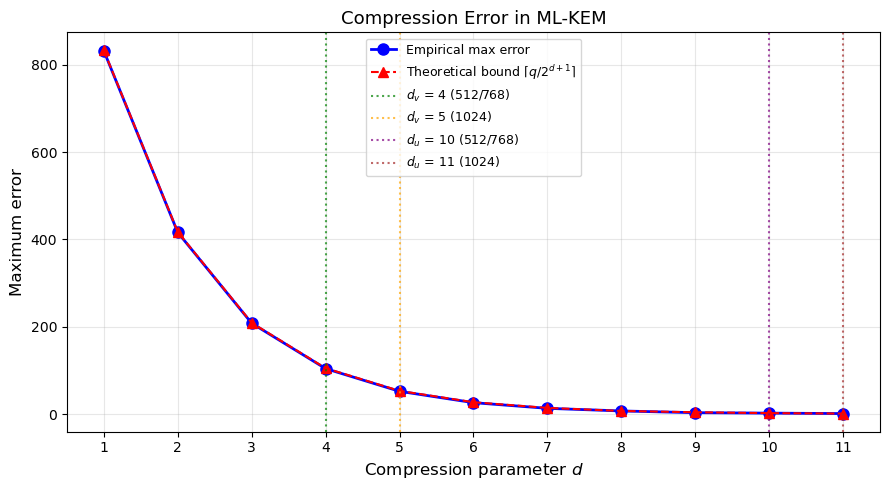
Max compression errors:
  d= 1: max_error= 832, bound= 833
  d= 2: max_error= 416, bound= 417
  d= 3: max_error= 208, bound= 209
  d= 4: max_error= 104, bound= 105
  d= 5: max_error=  52, bound=  53
  d= 6: max_error=  26, bound=  27
  d= 7: max_error=  13, bound=  14
  d= 8: max_error=   7, bound=   7
  d= 9: max_error=   3, bound=   4
  d=10: max_error=   2, bound=   2
  d=11: max_error=   1, bound=   1
41.18 Summary#
In this chapter we built a complete educational implementation of ML-KEM (Kyber), the first NIST-standardised post-quantum key encapsulation mechanism:
Mathematical foundations: the polynomial ring \(R_q = \mathbb{Z}_{3329}[x]/(x^{256}+1)\), the Module-LWE problem, and the centered binomial distribution.
Number Theoretic Transform (NTT): forward and inverse transforms using Cooley-Tukey and Gentleman-Sande butterflies, achieving \(O(n \log n)\) polynomial multiplication with a measured speedup over schoolbook.
Full ML-KEM protocol: KeyGen, Encaps, and Decaps operations, demonstrating successful shared secret agreement across all three parameter sets.
Experimental analysis:
Decryption noise stays well within the correctness threshold.
All parameter sets achieve high success rate in our tests (theoretical failure probability is \(< 2^{-139}\) for ML-KEM-512).
Key and ciphertext sizes range from 800+768 bytes (ML-KEM-512) to 1568+1568 bytes (ML-KEM-1024).
Comparison with classical schemes: ML-KEM keys are larger than ECDH but still practical, and the scheme is already being deployed in TLS 1.3.
Key Takeaways#
ML-KEM’s security rests on the hardness of Module-LWE, which is believed to resist both classical and quantum attacks.
The NTT is the key algorithmic enabler, making polynomial ring operations fast.
The centered binomial distribution provides efficient, constant-time noise sampling.
Parameter selection balances security level, key sizes, and failure probability.
ML-KEM is already being adopted as a hybrid KEM (alongside X25519) in major internet protocols.
References#
NIST (2024). FIPS 203: Module-Lattice-Based Key-Encapsulation Mechanism Standard. https://csrc.nist.gov/pubs/fips/203/final
Avanzi, R., Bos, J., Ducas, L., Kiltz, E., Lepoint, T., Lyubashevsky, V., Schanck, J.M., Schwabe, P., Seiler, G., Stehle, D. (2021). CRYSTALS-Kyber: Algorithm Specifications and Supporting Documentation (version 3.02).
Regev, O. (2005). On Lattices, Learning with Errors, Random Linear Codes, and Cryptography. STOC 2005.
Lyubashevsky, V., Peikert, C., Regev, O. (2010). On Ideal Lattices and Learning with Errors Over Rings. EUROCRYPT 2010.
Langlois, A., Stehle, D. (2015). Worst-Case to Average-Case Reductions for Module Lattices. Designs, Codes and Cryptography.
Peikert, C. (2016). A Decade of Lattice Cryptography. Foundations and Trends in Theoretical Computer Science.
Bernstein, D.J., Lange, T. (2017). Post-quantum cryptography. Nature 549, 188–194.