
Chapter 20 – Difference Distribution and Differential Trails#
“We have developed a new type of cryptanalytic attack which can break the full 16-round DES … The attack is based on the concept of a differential.” – Eli Biham and Adi Shamir, Differential Cryptanalysis of DES-like Cryptosystems, 1991
In this chapter we formalise the concept of differential trails (also called differential characteristics) and show how to trace input differences through multiple rounds of a substitution-permutation network (SPN). We build on the Heys tutorial SPN from previous chapters and implement tools to discover and evaluate optimal differential trails.
20.1 Historical Context: From DES to Differential Trails#
In 1990, Eli Biham and Adi Shamir published their landmark paper on differential cryptanalysis, the first publicly known attack that could theoretically break the full 16-round DES faster than brute force.
The key insight was deceptively simple: instead of analysing individual plaintexts, analyse pairs of plaintexts with a known XOR difference \(\Delta P = P \oplus P^*\). If the cipher’s internal structure causes certain output differences \(\Delta C = C \oplus C^*\) to occur with probability higher than \(2^{-n}\), an attacker can exploit this bias to recover key bits.
Biham and Shamir’s attack on DES worked by tracing a differential trail through all 16 rounds of the Feistel network. At each round, the input difference to the F-function was constrained to pass through specific S-boxes with high-probability differential transitions. By carefully choosing which S-boxes were “active” (receiving non-zero input differences) and which output differences to predict, they constructed trails spanning the entire cipher.
Year |
Milestone |
|---|---|
1990 |
Biham & Shamir circulate differential cryptanalysis preprint |
1991 |
Full paper: 16-round DES broken with \(2^{47}\) chosen plaintexts |
1993 |
Coppersmith reveals IBM knew of the technique since the 1970s |
1994 |
Differential cryptanalysis extended to hash functions |
2002 |
Heys publishes accessible tutorial using a small SPN |
Important
The NSA’s involvement in DES design becomes clearer in hindsight: the S-boxes were specifically chosen to resist differential cryptanalysis, a technique that was classified at the time. Coppersmith later confirmed that IBM’s team had independently discovered the attack and hardened DES against it. The design criteria included minimising the maximum entry in each S-box’s difference distribution table.
The attack proceeds by tracing a differential trail – a sequence of XOR differences through each round of the cipher. At each S-box, the input difference maps to possible output differences with varying probabilities. The trail with the highest overall probability gives the attacker the best chance of recovering key material from the last round.
20.2 Formal Definitions#
We now establish the mathematical framework for differential trails through an SPN cipher with \(R\) rounds, \(n_s\) S-boxes per round, each operating on \(m\)-bit words.
Definition 20.1 – Differential Trail (Characteristic)
A differential trail through an \(R\)-round SPN is a sequence of difference patterns:
where \(\Delta X_r\) is the input difference to the S-box layer in round \(r\), and \(\Delta Y_r\) is the output difference from the S-box layer in round \(r\).
The relationship \(\Delta X_{r+1} = \pi(\Delta Y_r)\) holds for \(r < R-1\), where \(\pi\) is the bit permutation layer. Note that XOR with round keys does not affect the difference because \(\Delta(X \oplus K) = \Delta X\) when both members of the pair use the same key.
Definition 20.2 – Active S-box
An S-box is active in round \(r\) of a differential trail if its input difference \(\Delta x_i^{(r)}\) is non-zero. If \(\Delta x_i^{(r)} = 0\), the S-box is inactive and its output difference is guaranteed to be zero.
The number of active S-boxes in a trail is a key measure of the trail’s strength: more active S-boxes generally mean lower probability.
Definition 20.3 – Trail Probability
The probability of a differential trail \(\mathcal{T}\) is the product of the individual S-box differential probabilities across all active S-boxes:
where \(\mathcal{A}_r\) is the set of active S-box indices in round \(r\), and \(\Pr[\Delta x \to \Delta y]\) is the entry from the difference distribution table (DDT) of the S-box, divided by \(2^m\).
Theorem 20.1 – Key Cancellation in Differential Trails
In an SPN cipher where round keys are XORed before the S-box layer, the XOR difference at the input to any S-box layer is independent of the round key. That is:
Proof
Let \(X = P \oplus K\) and \(X^* = P^* \oplus K\) where \(K\) is the round key. Then:
since \(K \oplus K = 0\). This holds regardless of the key value, meaning the differential propagation through the S-box layer depends only on the plaintext difference, not on the key. \(\square\)
This is why differential cryptanalysis works: the attacker can predict difference propagation without knowing the key.
20.3 The Heys Tutorial SPN#
We use the same SPN from Heys’ tutorial, which has become the standard pedagogical example for both linear and differential cryptanalysis:
Block size: 16 bits (four 4-bit words)
S-box: 4-bit to 4-bit (shared across all positions)
Permutation: bit-level permutation after each S-box layer
Rounds: 4 rounds of substitution-permutation + final key mixing
Key: five 16-bit round keys \(K_1, \ldots, K_5\)
The last round omits the permutation (a common design choice that does not weaken the cipher but simplifies analysis).
import numpy as np

# -- Heys Tutorial SPN parameters --
SBOX = np.array([0xE, 0x4, 0xD, 0x1, 0x2, 0xF, 0xB, 0x8,
                 0x3, 0xA, 0x6, 0xC, 0x5, 0x9, 0x0, 0x7], dtype=np.uint8)

SBOX_INV = np.zeros(16, dtype=np.uint8)
SBOX_INV[SBOX] = np.arange(16, dtype=np.uint8)

PERM = np.array([0, 4, 8, 12, 1, 5, 9, 13, 2, 6, 10, 14, 3, 7, 11, 15], dtype=int)

PERM_INV = np.zeros(16, dtype=int)
PERM_INV[PERM] = np.arange(16, dtype=int)


def sbox_layer(state):
    """Apply S-box to each 4-bit nibble of a 16-bit integer."""
    out = 0
    for i in range(4):
        nibble = (state >> (4 * (3 - i))) & 0xF
        out |= int(SBOX[nibble]) << (4 * (3 - i))
    return out


def perm_layer(state):
    """Apply bit permutation to a 16-bit integer."""
    out = 0
    for i in range(16):
        bit = (state >> (15 - i)) & 1
        out |= bit << (15 - PERM[i])
    return out


def spn_encrypt(plaintext, round_keys):
    """Encrypt a 16-bit plaintext through the 4-round SPN."""
    state = plaintext ^ round_keys[0]
    for r in range(1, 4):
        state = sbox_layer(state)
        state = perm_layer(state)
        state = state ^ round_keys[r]
    # Last round: S-box + key mixing (no permutation)
    state = sbox_layer(state)
    state = state ^ round_keys[4]
    return state


def spn_partial(plaintext, round_keys, n_rounds=2):
    """Encrypt through n_rounds of sub-perm-key.
    Returns state before the next round's S-box layer."""
    state = plaintext ^ round_keys[0]
    for r in range(1, n_rounds + 1):
        state = sbox_layer(state)
        state = perm_layer(state)
        state = state ^ round_keys[r]
    return state


# Quick test
rng = np.random.default_rng(42)
keys = rng.integers(0, 0x10000, size=5)
pt = 0xABCD
ct = spn_encrypt(pt, keys)
print(f'SPN loaded successfully.')
print(f'S-box:       {[hex(x) for x in SBOX]}')
print(f'Permutation: {list(PERM)}')
print(f'Test: encrypt(0x{pt:04X}) = 0x{ct:04X}')
SPN loaded successfully.
S-box:       ['0xe', '0x4', '0xd', '0x1', '0x2', '0xf', '0xb', '0x8', '0x3', '0xa', '0x6', '0xc', '0x5', '0x9', '0x0', '0x7']
Permutation: [0, 4, 8, 12, 1, 5, 9, 13, 2, 6, 10, 14, 3, 7, 11, 15]
Test: encrypt(0xABCD) = 0x450B
20.4 Difference Distribution Table#
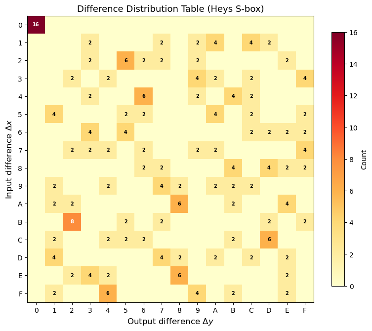
The difference distribution table (DDT) of the S-box is the foundation of differential cryptanalysis. For each input difference \(\Delta x\) and output difference \(\Delta y\), the DDT entry counts how many input values \(x \in \{0, \ldots, 2^m - 1\}\) satisfy \(S(x) \oplus S(x \oplus \Delta x) = \Delta y\).
Show code cell source
import numpy as np
import matplotlib.pyplot as plt

SBOX = np.array([0xE, 0x4, 0xD, 0x1, 0x2, 0xF, 0xB, 0x8,
                 0x3, 0xA, 0x6, 0xC, 0x5, 0x9, 0x0, 0x7], dtype=np.uint8)


def compute_ddt(sbox):
    """Compute the Difference Distribution Table for a 4-bit S-box."""
    n = len(sbox)
    ddt = np.zeros((n, n), dtype=int)
    for dx in range(n):
        for x in range(n):
            dy = int(sbox[x]) ^ int(sbox[x ^ dx])
            ddt[dx, dy] += 1
    return ddt


DDT = compute_ddt(SBOX)

fig, ax = plt.subplots(figsize=(8, 7))
im = ax.imshow(DDT, cmap='YlOrRd', interpolation='nearest')
ax.set_xlabel(r'Output difference $\Delta y$', fontsize=12)
ax.set_ylabel(r'Input difference $\Delta x$', fontsize=12)
ax.set_title('Difference Distribution Table (Heys S-box)', fontsize=13)
ax.set_xticks(range(16))
ax.set_yticks(range(16))
ax.set_xticklabels([f'{i:X}' for i in range(16)])
ax.set_yticklabels([f'{i:X}' for i in range(16)])

for i in range(16):
    for j in range(16):
        val = DDT[i, j]
        if val > 0:
            color = 'white' if val >= 8 else 'black'
            ax.text(j, i, str(val), ha='center', va='center',
                    fontsize=7, color=color, fontweight='bold')

plt.colorbar(im, ax=ax, label='Count', shrink=0.8)
plt.tight_layout()
plt.savefig('ch20_ddt_heatmap.png', dpi=150, bbox_inches='tight')
plt.show()

print(f'DDT shape: {DDT.shape}')
print(f'Row 0 (zero input diff): {DDT[0]}')
print(f'Max non-trivial entry: {DDT[1:, :].max()}')
print(f'Differential uniformity: {DDT[1:, :].max()}')
print(f'Entries with count >= 6: {np.sum(DDT[1:, :] >= 6)}')
DDT shape: (16, 16)
Row 0 (zero input diff): [16  0  0  0  0  0  0  0  0  0  0  0  0  0  0  0]
Max non-trivial entry: 8
Differential uniformity: 8
Entries with count >= 6: 7
20.5 Implementation: Differential#
Trail Class
We now build the DifferentialTrail class that traces a specific input
difference through the Heys SPN. The class validates trail consistency
(permuted outputs of round \(r\) must equal inputs of round \(r+1\)),
computes the trail probability, and counts active S-boxes.
import numpy as np

SBOX = np.array([0xE, 0x4, 0xD, 0x1, 0x2, 0xF, 0xB, 0x8,
                 0x3, 0xA, 0x6, 0xC, 0x5, 0x9, 0x0, 0x7], dtype=np.uint8)
PERM = np.array([0, 4, 8, 12, 1, 5, 9, 13, 2, 6, 10, 14, 3, 7, 11, 15], dtype=int)


def compute_ddt(sbox):
    n = len(sbox)
    ddt = np.zeros((n, n), dtype=int)
    for dx in range(n):
        for x in range(n):
            dy = int(sbox[x]) ^ int(sbox[x ^ dx])
            ddt[dx, dy] += 1
    return ddt


DDT = compute_ddt(SBOX)


def int_to_bits(val, n=16):
    """Convert integer to bit array (MSB first)."""
    return np.array([(val >> (n - 1 - i)) & 1 for i in range(n)], dtype=int)


def bits_to_int(bits):
    """Convert bit array to integer."""
    val = 0
    for b in bits:
        val = (val << 1) | int(b)
    return val


def apply_perm_to_bits(bits, perm):
    """Apply bit permutation: output[perm[i]] = input[i]."""
    out = np.zeros_like(bits)
    for i in range(len(perm)):
        out[perm[i]] = bits[i]
    return out


def perm_16bit(val):
    """Apply bit permutation to 16-bit value."""
    bits = int_to_bits(val)
    pbits = apply_perm_to_bits(bits, PERM)
    return bits_to_int(pbits)


def get_nibbles(val_16bit):
    """Extract four 4-bit nibbles from a 16-bit value."""
    return [(val_16bit >> (4 * (3 - i))) & 0xF for i in range(4)]


def nibbles_to_int(nibbles):
    """Combine four nibbles into a 16-bit integer."""
    return (nibbles[0] << 12) | (nibbles[1] << 8) | (nibbles[2] << 4) | nibbles[3]


class DifferentialTrail:
    """Represents and evaluates a differential trail through the Heys SPN.

    A trail specifies:
      - Input difference delta_P (16 bits)
      - For each round: the S-box output differences (4 nibbles)
    """

    def __init__(self, delta_p, round_outputs):
        """
        Parameters
        ----------
        delta_p : int
            16-bit input difference.
        round_outputs : list of lists
            Each inner list has 4 nibble values: the S-box output
            differences for that round.
        """
        self.delta_p = delta_p
        self.round_outputs = round_outputs
        self.n_rounds = len(round_outputs)
        self._validate()

    def _validate(self):
        """Validate trail consistency against DDT and permutation."""
        current_input = self.delta_p
        self.round_inputs = [current_input]
        self.active_sboxes = []

        for r in range(self.n_rounds):
            in_nibbles = get_nibbles(current_input)
            out_nibbles = self.round_outputs[r]
            active = []

            for i in range(4):
                if in_nibbles[i] == 0:
                    assert out_nibbles[i] == 0, (
                        f'Round {r+1}, S-box {i}: zero input but non-zero output'
                    )
                else:
                    assert DDT[in_nibbles[i], out_nibbles[i]] > 0, (
                        f'Round {r+1}, S-box {i}: '
                        f'DDT[0x{in_nibbles[i]:X}, 0x{out_nibbles[i]:X}] = 0'
                    )
                    active.append(i)

            self.active_sboxes.append(active)

            # Apply permutation to get next round input
            out_16 = nibbles_to_int(out_nibbles)
            out_bits = int_to_bits(out_16)
            perm_bits = apply_perm_to_bits(out_bits, PERM)
            current_input = bits_to_int(perm_bits)
            if r < self.n_rounds - 1:
                self.round_inputs.append(current_input)

        self.delta_u_final = current_input

    def probability(self):
        """Product of S-box differential probabilities."""
        prob = 1.0
        for r in range(self.n_rounds):
            in_nibbles = get_nibbles(self.round_inputs[r])
            out_nibbles = self.round_outputs[r]
            for i in self.active_sboxes[r]:
                count = DDT[in_nibbles[i], out_nibbles[i]]
                prob *= count / 16.0
        return prob

    def total_active(self):
        """Total number of active S-boxes across all rounds."""
        return sum(len(a) for a in self.active_sboxes)

    def summary(self):
        """Return a summary string."""
        lines = []
        lines.append(f'Differential Trail: dP = 0x{self.delta_p:04X}')
        lines.append(f'  Output after last perm: dU = 0x{self.delta_u_final:04X}')
        lines.append(f'  Probability: {float(self.probability()):.6f}')
        lines.append(f'  Total active S-boxes: {self.total_active()}')
        for r in range(self.n_rounds):
            in_nibs = get_nibbles(self.round_inputs[r])
            out_nibs = self.round_outputs[r]
            active = self.active_sboxes[r]
            parts = []
            for i in active:
                p = DDT[in_nibs[i], out_nibs[i]] / 16.0
                parts.append(f'S{i}: 0x{in_nibs[i]:X}->0x{out_nibs[i]:X} '
                             f'(p={float(p):.4f})')
            lines.append(f'  Round {r+1}: input=0x{self.round_inputs[r]:04X}  '
                         f'active={active}  {", ".join(parts)}')
        return '\n'.join(lines)


print('DifferentialTrail class defined.')
print(f'Utility functions: int_to_bits, bits_to_int, perm_16bit, '
      f'get_nibbles, nibbles_to_int')
DifferentialTrail class defined.
Utility functions: int_to_bits, bits_to_int, perm_16bit, get_nibbles, nibbles_to_int
20.6 Tracing the Heys Differential Trail#
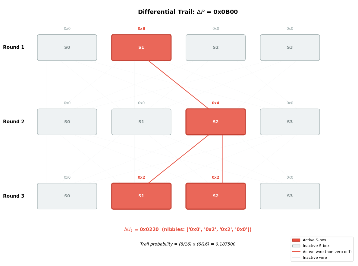
The classic Heys differential trail uses input difference \(\Delta P = \texttt{0x0B00}\), which activates only one S-box per round for the first two rounds. The corresponding bit pattern is:
Let us trace this trail step by step through the permutation and DDT.
import numpy as np

SBOX = np.array([0xE, 0x4, 0xD, 0x1, 0x2, 0xF, 0xB, 0x8,
                 0x3, 0xA, 0x6, 0xC, 0x5, 0x9, 0x0, 0x7], dtype=np.uint8)
PERM = np.array([0, 4, 8, 12, 1, 5, 9, 13, 2, 6, 10, 14, 3, 7, 11, 15], dtype=int)


def compute_ddt(sbox):
    n = len(sbox)
    ddt = np.zeros((n, n), dtype=int)
    for dx in range(n):
        for x in range(n):
            dy = int(sbox[x]) ^ int(sbox[x ^ dx])
            ddt[dx, dy] += 1
    return ddt


DDT = compute_ddt(SBOX)


def int_to_bits(val, n=16):
    return np.array([(val >> (n - 1 - i)) & 1 for i in range(n)], dtype=int)


def bits_to_int(bits):
    val = 0
    for b in bits:
        val = (val << 1) | int(b)
    return val


def apply_perm_to_bits(bits, perm):
    out = np.zeros_like(bits)
    for i in range(len(perm)):
        out[perm[i]] = bits[i]
    return out


def perm_16bit(val):
    bits = int_to_bits(val)
    pbits = apply_perm_to_bits(bits, PERM)
    return bits_to_int(pbits)


def get_nibbles(val):
    return [(val >> (4 * (3 - i))) & 0xF for i in range(4)]


def nibbles_to_int(nibs):
    return (nibs[0] << 12) | (nibs[1] << 8) | (nibs[2] << 4) | nibs[3]


# -- Trace step by step --
print('=' * 65)
print('TRACING THE HEYS DIFFERENTIAL TRAIL')
print('=' * 65)

delta_p = 0x0B00
print(f'\nInput difference: dP = 0x{delta_p:04X}')
print(f'  Nibbles: {[f"0x{n:X}" for n in get_nibbles(delta_p)]}')
print(f'  Binary:  {list(int_to_bits(delta_p))}')

# Round 1: S-box 1 has input diff 0xB -> output 0x2 (count=8)
print(f'\n--- Round 1 ---')
print(f'  DDT row for dx=0xB: {DDT[0xB]}')
r1_sbox_out = [0, 0x2, 0, 0]
r1_out_16 = nibbles_to_int(r1_sbox_out)
r1_perm = perm_16bit(r1_out_16)
print(f'  S-box output: {[f"0x{n:X}" for n in r1_sbox_out]}')
print(f'  DDT[0xB, 0x2] = {DDT[0xB, 0x2]}, prob = {DDT[0xB, 0x2]/16}')
print(f'  After permutation: 0x{r1_perm:04X}')
print(f'  Perm output bits: {list(int_to_bits(r1_perm))}')

# Round 2
r2_nibs = get_nibbles(r1_perm)
active_r2 = [i for i in range(4) if r2_nibs[i] != 0]
print(f'\n--- Round 2 ---')
print(f'  Input: 0x{r1_perm:04X}, nibbles: {[f"0x{n:X}" for n in r2_nibs]}')
print(f'  Active S-boxes: {active_r2}')

dx2 = r2_nibs[active_r2[0]]
print(f'  DDT row for dx=0x{dx2:X}: {DDT[dx2]}')
best_dy2 = max(range(1, 16), key=lambda dy: DDT[dx2, dy])
print(f'  Best output: dy=0x{best_dy2:X} with count={DDT[dx2, best_dy2]}')

r2_sbox_out = [0, 0, 0, 0]
r2_sbox_out[active_r2[0]] = best_dy2
r2_out_16 = nibbles_to_int(r2_sbox_out)
r2_perm = perm_16bit(r2_out_16)
print(f'  S-box output: {[f"0x{n:X}" for n in r2_sbox_out]}')
print(f'  After permutation: 0x{r2_perm:04X}')

# Round 3 input (= dU at input to last-round S-boxes)
r3_nibs = get_nibbles(r2_perm)
active_r3 = [i for i in range(4) if r3_nibs[i] != 0]
print(f'\n--- Round 3 (input to last-round S-boxes) ---')
print(f'  dU = 0x{r2_perm:04X}, nibbles: {[f"0x{n:X}" for n in r3_nibs]}')
print(f'  Active S-boxes: {active_r3}')
print(f'  Binary: {list(int_to_bits(r2_perm))}')

# Overall probability
prob = (DDT[0xB, 0x2] / 16.0) * (DDT[dx2, best_dy2] / 16.0)
print(f'\nTrail probability (rounds 1-2):')
print(f'  = ({DDT[0xB, 0x2]}/16) * ({DDT[dx2, best_dy2]}/16)')
print(f'  = {float(DDT[0xB, 0x2]/16):.4f} * {float(DDT[dx2, best_dy2]/16):.4f}')
print(f'  = {float(prob):.6f}')
print(f'\nExpected: (8/16)*(6/16) = {float((8/16)*(6/16)):.6f}')
=================================================================
TRACING THE HEYS DIFFERENTIAL TRAIL
=================================================================

Input difference: dP = 0x0B00
  Nibbles: ['0x0', '0xB', '0x0', '0x0']
  Binary:  [0, 0, 0, 0, 1, 0, 1, 1, 0, 0, 0, 0, 0, 0, 0, 0]

--- Round 1 ---
  DDT row for dx=0xB: [0 0 8 0 0 2 0 2 0 0 0 0 0 2 0 2]
  S-box output: ['0x0', '0x2', '0x0', '0x0']
  DDT[0xB, 0x2] = 8, prob = 0.5
  After permutation: 0x0040
  Perm output bits: [0, 0, 0, 0, 0, 0, 0, 0, 0, 1, 0, 0, 0, 0, 0, 0]

--- Round 2 ---
  Input: 0x0040, nibbles: ['0x0', '0x0', '0x4', '0x0']
  Active S-boxes: [2]
  DDT row for dx=0x4: [0 0 0 2 0 0 6 0 0 2 0 4 2 0 0 0]
  Best output: dy=0x6 with count=6
  S-box output: ['0x0', '0x0', '0x6', '0x0']
  After permutation: 0x0220

--- Round 3 (input to last-round S-boxes) ---
  dU = 0x0220, nibbles: ['0x0', '0x2', '0x2', '0x0']
  Active S-boxes: [1, 2]
  Binary: [0, 0, 0, 0, 0, 0, 1, 0, 0, 0, 1, 0, 0, 0, 0, 0]

Trail probability (rounds 1-2):
  = (8/16) * (6/16)
  = 0.5000 * 0.3750
  = 0.187500

Expected: (8/16)*(6/16) = 0.187500
The Standard Heys Trail
The trail uses input difference \(\Delta P = \texttt{0x0B00}\), which activates only one S-box per round for two consecutive rounds. The first active S-box has DDT entry \(8/16 = 0.5\) (for \(\Delta x = \texttt{0xB} \to \Delta y = \texttt{0x2}\)) and the second has \(6/16 = 0.375\) (for \(\Delta x = \texttt{0x4} \to \Delta y = \texttt{0x6}\)), giving an overall trail probability of \((8/16)(6/16) = 3/16 = 0.1875\). This is remarkably high for a 2-round trail and enables practical key recovery.
20.7 Visualizing the Trail Through the SPN#
The following visualization shows the differential trail propagating through the SPN. Active S-boxes are highlighted in red, and active wires (carrying non-zero differences) are shown in red through the permutation layer.
Show code cell source
import numpy as np
import matplotlib.pyplot as plt
import matplotlib.patches as mpatches

SBOX = np.array([0xE, 0x4, 0xD, 0x1, 0x2, 0xF, 0xB, 0x8,
                 0x3, 0xA, 0x6, 0xC, 0x5, 0x9, 0x0, 0x7], dtype=np.uint8)
PERM = np.array([0, 4, 8, 12, 1, 5, 9, 13, 2, 6, 10, 14, 3, 7, 11, 15], dtype=int)


def compute_ddt(sbox):
    n = len(sbox)
    ddt = np.zeros((n, n), dtype=int)
    for dx in range(n):
        for x in range(n):
            dy = int(sbox[x]) ^ int(sbox[x ^ dx])
            ddt[dx, dy] += 1
    return ddt


DDT = compute_ddt(SBOX)


def int_to_bits(val, n=16):
    return np.array([(val >> (n - 1 - i)) & 1 for i in range(n)], dtype=int)


def bits_to_int(bits):
    val = 0
    for b in bits:
        val = (val << 1) | int(b)
    return val


def apply_perm_to_bits(bits, perm):
    out = np.zeros_like(bits)
    for i in range(len(perm)):
        out[perm[i]] = bits[i]
    return out


def perm_16bit(val):
    bits = int_to_bits(val)
    pbits = apply_perm_to_bits(bits, PERM)
    return bits_to_int(pbits)


def get_nibbles(val):
    return [(val >> (4 * (3 - i))) & 0xF for i in range(4)]


def nibbles_to_int(nibs):
    return (nibs[0] << 12) | (nibs[1] << 8) | (nibs[2] << 4) | nibs[3]


# -- Compute trail differences --
r1_in = 0x0B00
r1_nibs_in = get_nibbles(r1_in)
r1_sbox_out = [0, 0x2, 0, 0]
r1_perm = perm_16bit(nibbles_to_int(r1_sbox_out))

r2_nibs_in = get_nibbles(r1_perm)
active_r2_idx = [i for i in range(4) if r2_nibs_in[i] != 0][0]
dx_r2 = r2_nibs_in[active_r2_idx]
best_dy_r2 = max(range(1, 16), key=lambda dy: DDT[dx_r2, dy])

r2_sbox_out = [0, 0, 0, 0]
r2_sbox_out[active_r2_idx] = best_dy_r2
r2_perm = perm_16bit(nibbles_to_int(r2_sbox_out))
r3_nibs_in = get_nibbles(r2_perm)

trail_data = {
    'round_inputs': [r1_nibs_in, r2_nibs_in, r3_nibs_in],
    'round_sbox_outputs': [r1_sbox_out, r2_sbox_out, r3_nibs_in],
    'active': [
        [i for i in range(4) if r1_nibs_in[i] != 0],
        [i for i in range(4) if r2_nibs_in[i] != 0],
        [i for i in range(4) if r3_nibs_in[i] != 0],
    ]
}

# -- Visualization --
fig, ax = plt.subplots(figsize=(12, 10))
ax.set_xlim(-1, 17)
ax.set_ylim(-1, 13)
ax.set_aspect('equal')
ax.axis('off')

color_active = '#e74c3c'
color_inactive = '#ecf0f1'
color_wire_active = '#e74c3c'
color_wire_inactive = '#bdc3c7'

sbox_w, sbox_h = 3.0, 1.2
x_positions = [0, 4, 8, 12]
round_labels = ['Round 1', 'Round 2', 'Round 3']
y_positions = [10, 6, 2]

ax.text(8, 12.5,
        r'Differential Trail: $\Delta P$ = 0x' + f'{r1_in:04X}',
        ha='center', va='center', fontsize=14, fontweight='bold')

for r_idx in range(3):
    y = y_positions[r_idx]
    in_nibs = trail_data['round_inputs'][r_idx]
    active = trail_data['active'][r_idx]

    ax.text(-0.8, y + sbox_h / 2, round_labels[r_idx],
            ha='right', va='center', fontsize=11, fontweight='bold')

    for s in range(4):
        x = x_positions[s]
        is_active = s in active

        fc = color_active if is_active else color_inactive
        ec = '#c0392b' if is_active else '#95a5a6'
        lw = 2.5 if is_active else 1.0
        rect = mpatches.FancyBboxPatch(
            (x, y), sbox_w, sbox_h,
            boxstyle='round,pad=0.1',
            facecolor=fc, edgecolor=ec, linewidth=lw, alpha=0.85
        )
        ax.add_patch(rect)

        label = f'S{s}'
        tcolor = 'white' if is_active else '#7f8c8d'
        ax.text(x + sbox_w / 2, y + sbox_h / 2, label,
                ha='center', va='center', fontsize=10, fontweight='bold',
                color=tcolor)

        diff_val = in_nibs[s]
        ax.text(x + sbox_w / 2, y + sbox_h + 0.3,
                f'0x{diff_val:X}', ha='center', va='bottom',
                fontsize=9,
                color=color_active if is_active else '#95a5a6',
                fontweight='bold' if is_active else 'normal')

    # Draw permutation wires between rounds
    if r_idx < 2:
        out_nibs = trail_data['round_sbox_outputs'][r_idx]
        y_bot = y
        y_top_next = y_positions[r_idx + 1] + sbox_h

        for s_from in range(4):
            for bit_in_nibble in range(4):
                global_bit = s_from * 4 + bit_in_nibble
                target_bit = PERM[global_bit]
                s_to = target_bit // 4
                bit_in_target = target_bit % 4

                x_start = x_positions[s_from] + (bit_in_nibble + 0.5) * (sbox_w / 4)
                x_end = x_positions[s_to] + (bit_in_target + 0.5) * (sbox_w / 4)

                out_bits = int_to_bits(nibbles_to_int(out_nibs))
                wire_active = out_bits[global_bit] == 1

                wcolor = color_wire_active if wire_active else color_wire_inactive
                walpha = 0.9 if wire_active else 0.15
                wlw = 1.8 if wire_active else 0.4

                ax.plot([x_start, x_end],
                        [y_bot - 0.1, y_top_next + 0.1],
                        color=wcolor, alpha=walpha, linewidth=wlw)

# Output label
ax.text(8, 0.8,
        r'$\Delta U_3$ = 0x' + f'{nibbles_to_int(r3_nibs_in):04X}'
        + f'  (nibbles: {[f"0x{n:X}" for n in r3_nibs_in]})',
        ha='center', va='center', fontsize=11, fontweight='bold',
        color=color_active)

prob = (DDT[0xB, 0x2] / 16) * (DDT[dx_r2, best_dy_r2] / 16)
ax.text(8, 0.0,
        f'Trail probability = '
        f'({DDT[0xB,0x2]}/16) x ({DDT[dx_r2,best_dy_r2]}/16) = {float(prob):.6f}',
        ha='center', va='center', fontsize=10, style='italic')

legend_elements = [
    mpatches.Patch(facecolor=color_active, edgecolor='#c0392b',
                   label='Active S-box'),
    mpatches.Patch(facecolor=color_inactive, edgecolor='#95a5a6',
                   label='Inactive S-box'),
    plt.Line2D([0], [0], color=color_wire_active, linewidth=2,
               label='Active wire (non-zero diff)'),
    plt.Line2D([0], [0], color=color_wire_inactive, linewidth=1,
               alpha=0.4, label='Inactive wire'),
]
ax.legend(handles=legend_elements, loc='lower right', fontsize=9,
          framealpha=0.9)

plt.tight_layout()
plt.savefig('ch20_trail_visualization.png', dpi=150, bbox_inches='tight')
plt.show()

total_active = sum(len(a) for a in trail_data['active'])
print(f'Trail visualized: {total_active} total active S-boxes across 3 rounds')
Trail visualized: 4 total active S-boxes across 3 rounds
20.8 Experimental Verification of Trail Probability#
We now verify the trail probability experimentally. For many random keys, we encrypt pairs \((P, P^*)\) with \(P^* = P \oplus \Delta P\) through the first two rounds and check whether the output difference matches the predicted \(\Delta U\). The theoretical trail probability is \((8/16)(6/16) = 3/16 = 0.1875\).
Show code cell source
import numpy as np
import matplotlib.pyplot as plt

SBOX = np.array([0xE, 0x4, 0xD, 0x1, 0x2, 0xF, 0xB, 0x8,
                 0x3, 0xA, 0x6, 0xC, 0x5, 0x9, 0x0, 0x7], dtype=np.uint8)
PERM = np.array([0, 4, 8, 12, 1, 5, 9, 13, 2, 6, 10, 14, 3, 7, 11, 15], dtype=int)


def sbox_layer(state):
    out = 0
    for i in range(4):
        nibble = (state >> (4 * (3 - i))) & 0xF
        out |= int(SBOX[nibble]) << (4 * (3 - i))
    return out


def perm_layer(state):
    out = 0
    for i in range(16):
        bit = (state >> (15 - i)) & 1
        out |= bit << (15 - PERM[i])
    return out


def spn_partial(plaintext, round_keys, n_rounds=2):
    """Encrypt through n_rounds of sub-perm-key."""
    state = plaintext ^ round_keys[0]
    for r in range(1, n_rounds + 1):
        state = sbox_layer(state)
        state = perm_layer(state)
        state = state ^ round_keys[r]
    return state


def compute_ddt(sbox):
    n = len(sbox)
    ddt = np.zeros((n, n), dtype=int)
    for dx in range(n):
        for x in range(n):
            dy = int(sbox[x]) ^ int(sbox[x ^ dx])
            ddt[dx, dy] += 1
    return ddt


DDT = compute_ddt(SBOX)


def int_to_bits(val, n=16):
    return np.array([(val >> (n - 1 - i)) & 1 for i in range(n)], dtype=int)


def bits_to_int(bits):
    val = 0
    for b in bits:
        val = (val << 1) | int(b)
    return val


def apply_perm_to_bits(bits, perm):
    out = np.zeros_like(bits)
    for i in range(len(perm)):
        out[perm[i]] = bits[i]
    return out


def perm_16bit(val):
    bits = int_to_bits(val)
    pbits = apply_perm_to_bits(bits, PERM)
    return bits_to_int(pbits)


def get_nibbles(val):
    return [(val >> (4 * (3 - i))) & 0xF for i in range(4)]


def nibbles_to_int(nibs):
    return (nibs[0] << 12) | (nibs[1] << 8) | (nibs[2] << 4) | nibs[3]


# Compute target delta_u from the trail
r1_out = nibbles_to_int([0, 0x2, 0, 0])
r1_perm = perm_16bit(r1_out)
r2_nibs = get_nibbles(r1_perm)
active_idx = [i for i in range(4) if r2_nibs[i] != 0][0]
dx2 = r2_nibs[active_idx]
best_dy2 = max(range(1, 16), key=lambda dy: DDT[dx2, dy])
r2_out = [0, 0, 0, 0]
r2_out[active_idx] = best_dy2
r2_perm = perm_16bit(nibbles_to_int(r2_out))
target_delta_u = r2_perm

trail_prob_theory = (DDT[0xB, 0x2] / 16) * (DDT[dx2, best_dy2] / 16)
print(f'Target delta_U: 0x{target_delta_u:04X}')
print(f'Theoretical trail probability: {float(trail_prob_theory):.6f}')

# -- Experiment --
rng = np.random.default_rng(2024)
delta_p = 0x0B00
n_keys_exp = 500
n_pairs = 10000
key_probs = np.zeros(n_keys_exp)

for k_idx in range(n_keys_exp):
    keys = rng.integers(0, 0x10000, size=5)
    count = 0
    for _ in range(n_pairs):
        p = rng.integers(0, 0x10000)
        p_star = p ^ delta_p
        u = spn_partial(p, keys, 2)
        u_star = spn_partial(p_star, keys, 2)
        if (u ^ u_star) == target_delta_u:
            count += 1
    key_probs[k_idx] = count / n_pairs

avg = np.mean(key_probs)
std = np.std(key_probs)

fig, (ax1, ax2) = plt.subplots(1, 2, figsize=(13, 5))

ax1.hist(key_probs, bins=30, color='#3498db', edgecolor='black',
         alpha=0.8, density=True)
ax1.axvline(trail_prob_theory, color='#e74c3c', linewidth=2,
            linestyle='--',
            label=f'Theory = {float(trail_prob_theory):.4f}')
ax1.axvline(avg, color='#2ecc71', linewidth=2, linestyle='-',
            label=f'Exp mean = {float(avg):.4f}')
ax1.set_xlabel('Observed Probability', fontsize=12)
ax1.set_ylabel('Density', fontsize=12)
ax1.set_title(
    f'Trail Probability Distribution\n'
    f'({n_keys_exp} random keys, {n_pairs} pairs each)', fontsize=12)
ax1.legend(fontsize=10)
ax1.grid(True, alpha=0.3)

running_avg = np.cumsum(key_probs) / np.arange(1, n_keys_exp + 1)
ax2.plot(range(1, n_keys_exp + 1), running_avg,
         color='#3498db', linewidth=1.5)
ax2.axhline(trail_prob_theory, color='#e74c3c', linewidth=2,
            linestyle='--',
            label=f'Theory = {float(trail_prob_theory):.4f}')
ax2.fill_between(range(1, n_keys_exp + 1),
                 trail_prob_theory - 0.01,
                 trail_prob_theory + 0.01,
                 color='#e74c3c', alpha=0.1)
ax2.set_xlabel('Number of Keys Tested', fontsize=12)
ax2.set_ylabel('Running Average Probability', fontsize=12)
ax2.set_title('Convergence of Experimental Probability', fontsize=12)
ax2.legend(fontsize=10)
ax2.grid(True, alpha=0.3)
ax2.set_xlim(1, n_keys_exp)

plt.tight_layout()
plt.savefig('ch20_trail_probability_experiment.png', dpi=150,
            bbox_inches='tight')
plt.show()

print(f'\nExperimental mean probability: {float(avg):.6f}')
print(f'Theoretical trail probability:  {float(trail_prob_theory):.6f}')
print(f'Standard deviation across keys: {float(std):.6f}')
print(f'Ratio (exp/theory): {float(avg / trail_prob_theory):.4f}')
Target delta_U: 0x0220
Theoretical trail probability: 0.187500
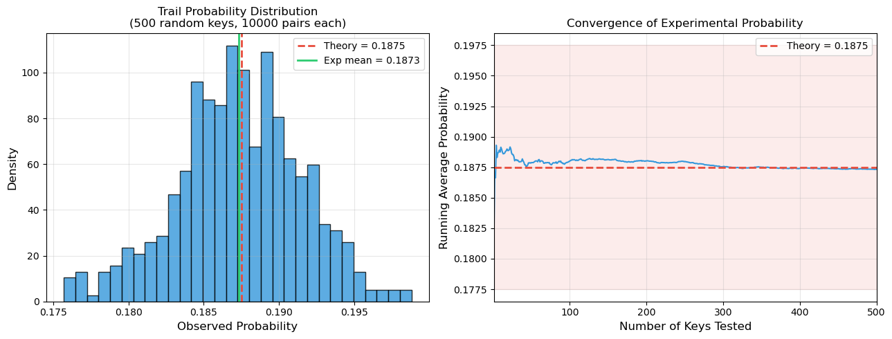
Experimental mean probability: 0.187331
Theoretical trail probability:  0.187500
Standard deviation across keys: 0.004161
Ratio (exp/theory): 0.9991
Trail vs. Differential
A trail (characteristic) specifies the exact difference at every intermediate point. A differential specifies only the input and output differences, summing over all possible trails that connect them. The experimental probability above may slightly exceed the single-trail prediction because multiple trails with the same \((\Delta P, \Delta U)\) can contribute. This is called the differential effect.
20.9 Trail#
Searcher: Finding Optimal Trails
To find the best differential trail, we search over all possible input differences and, for each active S-box in each round, all possible output differences. We prune branches whose cumulative probability falls below a threshold to keep the search tractable.
import numpy as np

SBOX = np.array([0xE, 0x4, 0xD, 0x1, 0x2, 0xF, 0xB, 0x8,
                 0x3, 0xA, 0x6, 0xC, 0x5, 0x9, 0x0, 0x7], dtype=np.uint8)
PERM = np.array([0, 4, 8, 12, 1, 5, 9, 13, 2, 6, 10, 14, 3, 7, 11, 15], dtype=int)


def compute_ddt(sbox):
    n = len(sbox)
    ddt = np.zeros((n, n), dtype=int)
    for dx in range(n):
        for x in range(n):
            dy = int(sbox[x]) ^ int(sbox[x ^ dx])
            ddt[dx, dy] += 1
    return ddt


DDT = compute_ddt(SBOX)


def int_to_bits(val, n=16):
    return np.array([(val >> (n - 1 - i)) & 1 for i in range(n)], dtype=int)


def bits_to_int(bits):
    val = 0
    for b in bits:
        val = (val << 1) | int(b)
    return val


def apply_perm_to_bits(bits, perm):
    out = np.zeros_like(bits)
    for i in range(len(perm)):
        out[perm[i]] = bits[i]
    return out


def perm_16bit(val):
    bits = int_to_bits(val)
    pbits = apply_perm_to_bits(bits, PERM)
    return bits_to_int(pbits)


def get_nibbles(val_16bit):
    return [(val_16bit >> (4 * (3 - i))) & 0xF for i in range(4)]


def nibbles_to_int(nibbles):
    return (nibbles[0] << 12) | (nibbles[1] << 8) | (nibbles[2] << 4) | nibbles[3]


class TrailSearcher:
    """Search for high-probability differential trails through the SPN."""

    def __init__(self, ddt, perm_func, n_sboxes=4, n_rounds=2):
        self.ddt = ddt
        self.perm = perm_func
        self.n_sboxes = n_sboxes
        self.n_rounds = n_rounds
        self.best_trails = []

    def _get_sbox_transitions(self, dx):
        """Return (dy, probability) pairs for non-zero dx."""
        transitions = []
        for dy in range(1, 16):
            count = self.ddt[dx, dy]
            if count > 0:
                transitions.append((dy, count / 16.0))
        return transitions

    def _search_round(self, input_diff, round_idx, current_prob,
                      trail_so_far, min_prob):
        """Recursively search from the given round."""
        nibbles = get_nibbles(input_diff)
        active_indices = [i for i in range(4) if nibbles[i] != 0]

        if len(active_indices) == 0:
            return

        all_transitions = []
        for idx in active_indices:
            trans = self._get_sbox_transitions(nibbles[idx])
            all_transitions.append((idx, trans))

        self._enumerate_combos(
            all_transitions, 0, nibbles, [0] * 4,
            round_idx, current_prob, trail_so_far, min_prob
        )

    def _enumerate_combos(self, transitions, t_idx, in_nibbles,
                          out_nibbles, round_idx, current_prob,
                          trail_so_far, min_prob):
        """Enumerate all S-box output combinations."""
        if t_idx == len(transitions):
            out_16 = nibbles_to_int(out_nibbles)
            next_input = self.perm(out_16)
            new_trail = trail_so_far + [
                (list(in_nibbles), list(out_nibbles))
            ]

            if round_idx == self.n_rounds - 1:
                self.best_trails.append(
                    (current_prob, new_trail, next_input)
                )
            else:
                self._search_round(
                    next_input, round_idx + 1,
                    current_prob, new_trail, min_prob
                )
            return

        sbox_idx, trans_list = transitions[t_idx]
        for dy, prob in trans_list:
            new_prob = current_prob * prob
            if new_prob < min_prob:
                continue
            new_out = list(out_nibbles)
            new_out[sbox_idx] = dy
            self._enumerate_combos(
                transitions, t_idx + 1, in_nibbles, new_out,
                round_idx, new_prob, trail_so_far, min_prob
            )

    def search(self, min_prob=1e-4, top_k=20):
        """Search all input differences for best trails."""
        self.best_trails = []
        for delta_p in range(1, 0x10000):
            self._search_round(delta_p, 0, 1.0, [], min_prob)
        self.best_trails.sort(key=lambda x: -x[0])
        return self.best_trails[:top_k]


# Run search
searcher = TrailSearcher(DDT, perm_16bit, n_rounds=2)
print('Searching for optimal 2-round differential trails...')
print('(pruning trails with probability < 0.01)')
top_trails = searcher.search(min_prob=0.01, top_k=15)

print(f'\nFound {len(searcher.best_trails)} trails above threshold.')
print(f'\nTop 15 trails:')
print(f'{"Rank":>4} {"Prob":>10} {"dP":>6} {"dU_out":>7} {"Active":>7}')
print('-' * 42)
for i, (prob, trail, delta_u) in enumerate(top_trails):
    dp_nibs = trail[0][0]
    dp_val = nibbles_to_int(dp_nibs)
    n_active = sum(
        1 for rnd in trail for j in range(4) if rnd[0][j] != 0
    )
    print(f'{i+1:>4} {float(prob):>10.6f} 0x{dp_val:04X} '
          f'0x{delta_u:04X} {n_active:>7}')
Searching for optimal 2-round differential trails...
(pruning trails with probability < 0.01)
Found 2011 trails above threshold.

Top 15 trails:
Rank       Prob     dP  dU_out  Active
------------------------------------------
   1   0.187500 0x00B0 0x0202       2
   2   0.187500 0x0B00 0x0220       2
   3   0.140625 0x00A0 0x0808       2
   4   0.140625 0x00E0 0x0808       2
   5   0.140625 0x00F0 0x0404       2
   6   0.140625 0x0A00 0x0880       2
   7   0.140625 0x0E00 0x0880       2
   8   0.140625 0x0F00 0x0440       2
   9   0.125000 0x000B 0x2020       2
  10   0.125000 0x000B 0x2200       2
  11   0.125000 0x0B00 0x2022       2
  12   0.125000 0xB000 0x2022       2
  13   0.125000 0xB000 0x2202       2
  14   0.093750 0x000A 0x8080       2
  15   0.093750 0x000A 0x8800       2
20.10 Active S-box Distribution#
The number of active S-boxes in a trail directly impacts its probability. Trails with fewer active S-boxes tend to have higher probability. Let us count the active S-boxes for the best greedy trail from each input difference and visualise the distribution.
Show code cell source
import numpy as np
import matplotlib.pyplot as plt

SBOX = np.array([0xE, 0x4, 0xD, 0x1, 0x2, 0xF, 0xB, 0x8,
                 0x3, 0xA, 0x6, 0xC, 0x5, 0x9, 0x0, 0x7], dtype=np.uint8)
PERM = np.array([0, 4, 8, 12, 1, 5, 9, 13, 2, 6, 10, 14, 3, 7, 11, 15], dtype=int)


def compute_ddt(sbox):
    n = len(sbox)
    ddt = np.zeros((n, n), dtype=int)
    for dx in range(n):
        for x in range(n):
            dy = int(sbox[x]) ^ int(sbox[x ^ dx])
            ddt[dx, dy] += 1
    return ddt


DDT = compute_ddt(SBOX)


def int_to_bits(val, n=16):
    return np.array([(val >> (n - 1 - i)) & 1 for i in range(n)], dtype=int)


def bits_to_int(bits):
    val = 0
    for b in bits:
        val = (val << 1) | int(b)
    return val


def apply_perm_to_bits(bits, perm):
    out = np.zeros_like(bits)
    for i in range(len(perm)):
        out[perm[i]] = bits[i]
    return out


def perm_16bit(val):
    bits = int_to_bits(val)
    pbits = apply_perm_to_bits(bits, PERM)
    return bits_to_int(pbits)


def get_nibbles(val):
    return [(val >> (4 * (3 - i))) & 0xF for i in range(4)]


def nibbles_to_int(nibs):
    return (nibs[0] << 12) | (nibs[1] << 8) | (nibs[2] << 4) | nibs[3]


# For each input difference, compute greedy best 2-round trail
results = []

for dp in range(1, 0x10000):
    nibs = get_nibbles(dp)
    active_r1 = [i for i in range(4) if nibs[i] != 0]
    n_active_r1 = len(active_r1)

    # Greedy: best output per active S-box in round 1
    out_nibs = [0, 0, 0, 0]
    prob_r1 = 1.0
    for i in active_r1:
        best_dy = max(range(1, 16), key=lambda dy: DDT[nibs[i], dy])
        out_nibs[i] = best_dy
        prob_r1 *= DDT[nibs[i], best_dy] / 16.0

    out_16 = nibbles_to_int(out_nibs)
    r2_input = perm_16bit(out_16)
    r2_nibs = get_nibbles(r2_input)
    active_r2 = [i for i in range(4) if r2_nibs[i] != 0]
    n_active_r2 = len(active_r2)

    prob_r2 = 1.0
    for i in active_r2:
        best_p = max(DDT[r2_nibs[i], dy] for dy in range(1, 16)) / 16.0
        prob_r2 *= best_p

    total_active = n_active_r1 + n_active_r2
    total_prob = prob_r1 * prob_r2
    results.append((dp, total_active, total_prob))

results_arr = np.array([(r[1], r[2]) for r in results])
active_counts = results_arr[:, 0].astype(int)
probs = results_arr[:, 1]

valid = probs > 0
active_valid = active_counts[valid]
probs_valid = probs[valid]

unique_active, counts = np.unique(active_valid, return_counts=True)

fig, (ax1, ax2) = plt.subplots(1, 2, figsize=(13, 5))

# Left: bar chart of active S-box counts
colors = ['#2ecc71' if u <= 3 else '#f39c12' if u <= 5
          else '#e74c3c' for u in unique_active]
ax1.bar(unique_active, counts, color=colors,
        edgecolor='black', linewidth=0.5)
ax1.set_xlabel('Number of Active S-boxes (2 rounds)', fontsize=12)
ax1.set_ylabel('Number of Input Differences', fontsize=12)
ax1.set_title('Distribution of Active S-box Counts\n'
              '(greedy best trail per input diff)', fontsize=12)
ax1.set_xticks(unique_active)
for u, c in zip(unique_active, counts):
    ax1.text(u, c + max(counts) * 0.02, str(c),
             ha='center', va='bottom', fontsize=9)

# Right: log probability vs active count
rng_plot = np.random.default_rng(42)
for n_act in sorted(np.unique(active_valid)):
    mask = active_valid == n_act
    p_subset = probs_valid[mask]
    if len(p_subset) > 500:
        idx = rng_plot.choice(len(p_subset), 500, replace=False)
        p_plot = p_subset[idx]
    else:
        p_plot = p_subset
    jitter = rng_plot.normal(0, 0.08, len(p_plot))
    ax2.scatter(np.full(len(p_plot), n_act) + jitter,
                np.log2(p_plot),
                alpha=0.2, s=6, color='#3498db')
    median_p = np.median(p_subset)
    ax2.scatter(n_act, np.log2(median_p), color='#e74c3c', s=80,
                marker='D', zorder=5, edgecolor='black', linewidth=0.5)

ax2.set_xlabel('Number of Active S-boxes', fontsize=12)
ax2.set_ylabel(r'$\log_2$(Trail Probability)', fontsize=12)
ax2.set_title('Trail Probability vs Active S-boxes\n'
              '(red diamonds = median)', fontsize=12)
ax2.grid(True, alpha=0.3)

plt.tight_layout()
plt.savefig('ch20_active_sbox_distribution.png', dpi=150,
            bbox_inches='tight')
plt.show()

print(f'Total input differences analysed: {len(results)}')
print(f'\nActive S-box count distribution:')
for u, c in zip(unique_active, counts):
    print(f'  {u} active: {c} input differences')
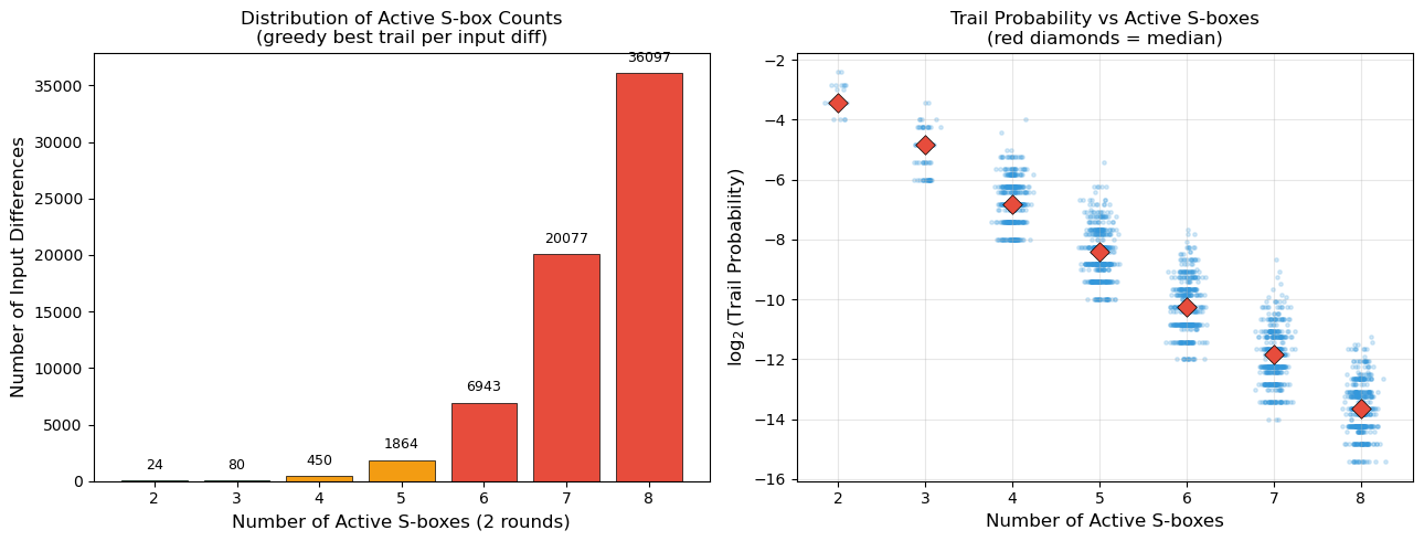
Total input differences analysed: 65535

Active S-box count distribution:
  2 active: 24 input differences
  3 active: 80 input differences
  4 active: 450 input differences
  5 active: 1864 input differences
  6 active: 6943 input differences
  7 active: 20077 input differences
  8 active: 36097 input differences
Observation
The scatter plot clearly shows the inverse relationship between the number of active S-boxes and the trail probability. Trails with only 2 active S-boxes achieve the highest probabilities (around \(\log_2(p) \approx -3\)), while trails with 6 or more active S-boxes have negligible probability. This explains why the Heys trail (2 active S-boxes) is so effective.
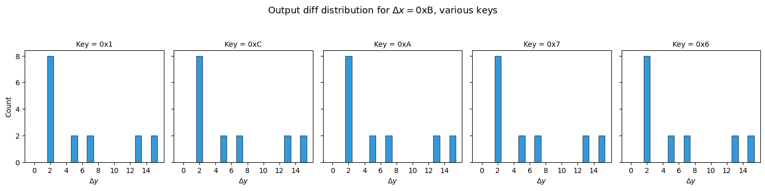
20.11 Verifying Key Cancellation (Theorem 20.1)#
Theorem 20.1 states that XOR differences at the S-box input are independent of the round key. We verify this experimentally: for a fixed input difference, the distribution of output differences after a single S-box should be identical regardless of the key nibble.
Show code cell source
import numpy as np
import matplotlib.pyplot as plt

SBOX = np.array([0xE, 0x4, 0xD, 0x1, 0x2, 0xF, 0xB, 0x8,
                 0x3, 0xA, 0x6, 0xC, 0x5, 0x9, 0x0, 0x7], dtype=np.uint8)

# S-box with input diff 0xB, under 5 different key nibbles
delta_x = 0xB
n_keys_test = 5
rng = np.random.default_rng(42)

fig, axes = plt.subplots(1, n_keys_test, figsize=(15, 3.5), sharey=True)

for k_idx in range(n_keys_test):
    key_nibble = rng.integers(0, 16)
    output_diff_counts = np.zeros(16, dtype=int)

    for x in range(16):
        x_keyed = x ^ key_nibble
        x_star_keyed = (x ^ delta_x) ^ key_nibble
        dy = int(SBOX[x_keyed]) ^ int(SBOX[x_star_keyed])
        output_diff_counts[dy] += 1

    axes[k_idx].bar(range(16), output_diff_counts, color='#3498db',
                    edgecolor='black', linewidth=0.5)
    axes[k_idx].set_xlabel(r'$\Delta y$', fontsize=10)
    axes[k_idx].set_title(f'Key = 0x{key_nibble:X}', fontsize=10)
    axes[k_idx].set_xticks(range(0, 16, 2))

    if k_idx == 0:
        axes[k_idx].set_ylabel('Count', fontsize=10)

fig.suptitle(
    r'Output diff distribution for $\Delta x = 0\mathrm{xB}$, '
    r'various keys',
    fontsize=13, y=1.05)

plt.tight_layout()
plt.savefig('ch20_key_cancellation.png', dpi=150, bbox_inches='tight')
plt.show()

print('All five histograms are IDENTICAL, confirming Theorem 20.1.')
print('The XOR difference at the S-box input depends only on the')
print('plaintext difference, not on the key value.')
All five histograms are IDENTICAL, confirming Theorem 20.1.
The XOR difference at the S-box input depends only on the
plaintext difference, not on the key value.
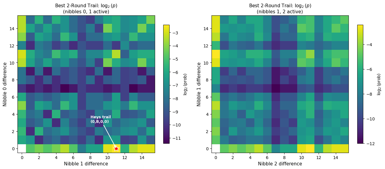
20.12 Differential Probability Landscape#
We visualise the best 2-round trail probability as a function of the input difference nibbles. We examine 2D slices where only two of the four nibbles are non-zero.
Show code cell source
import numpy as np
import matplotlib.pyplot as plt

SBOX = np.array([0xE, 0x4, 0xD, 0x1, 0x2, 0xF, 0xB, 0x8,
                 0x3, 0xA, 0x6, 0xC, 0x5, 0x9, 0x0, 0x7], dtype=np.uint8)
PERM = np.array([0, 4, 8, 12, 1, 5, 9, 13, 2, 6, 10, 14, 3, 7, 11, 15], dtype=int)


def compute_ddt(sbox):
    n = len(sbox)
    ddt = np.zeros((n, n), dtype=int)
    for dx in range(n):
        for x in range(n):
            dy = int(sbox[x]) ^ int(sbox[x ^ dx])
            ddt[dx, dy] += 1
    return ddt


DDT = compute_ddt(SBOX)


def int_to_bits(val, n=16):
    return np.array([(val >> (n - 1 - i)) & 1 for i in range(n)], dtype=int)


def bits_to_int(bits):
    val = 0
    for b in bits:
        val = (val << 1) | int(b)
    return val


def apply_perm_to_bits(bits, perm):
    out = np.zeros_like(bits)
    for i in range(len(perm)):
        out[perm[i]] = bits[i]
    return out


def perm_16bit(val):
    bits = int_to_bits(val)
    pbits = apply_perm_to_bits(bits, PERM)
    return bits_to_int(pbits)


def get_nibbles(val):
    return [(val >> (4 * (3 - i))) & 0xF for i in range(4)]


def best_2round_trail_prob(delta_p):
    """Greedy best 2-round trail probability."""
    nibs = get_nibbles(delta_p)
    if all(n == 0 for n in nibs):
        return 0.0
    active = [i for i in range(4) if nibs[i] != 0]
    out_nibs = [0] * 4
    prob_r1 = 1.0
    for i in active:
        best_dy = max(range(1, 16), key=lambda dy: DDT[nibs[i], dy])
        out_nibs[i] = best_dy
        prob_r1 *= DDT[nibs[i], best_dy] / 16.0
    out_16 = (out_nibs[0] << 12) | (out_nibs[1] << 8) | \
             (out_nibs[2] << 4) | out_nibs[3]
    r2_input = perm_16bit(out_16)
    r2_nibs = get_nibbles(r2_input)
    prob_r2 = 1.0
    for i in range(4):
        if r2_nibs[i] != 0:
            best_p = max(
                DDT[r2_nibs[i], dy] for dy in range(1, 16)
            ) / 16.0
            prob_r2 *= best_p
    return prob_r1 * prob_r2


# Compute for nibble0 x nibble1 (other nibbles = 0)
prob_matrix_01 = np.zeros((16, 16))
prob_matrix_12 = np.zeros((16, 16))

for n0 in range(16):
    for n1 in range(16):
        dp01 = (n0 << 12) | (n1 << 8)
        if dp01 > 0:
            prob_matrix_01[n0, n1] = best_2round_trail_prob(dp01)
        dp12 = (n1 << 8) | (n0 << 4)
        if dp12 > 0:
            prob_matrix_12[n1, n0] = best_2round_trail_prob(dp12)

fig, (ax1, ax2) = plt.subplots(1, 2, figsize=(13, 5.5))

log_01 = np.where(prob_matrix_01 > 0,
                  np.log2(prob_matrix_01), np.nan)
log_12 = np.where(prob_matrix_12 > 0,
                  np.log2(prob_matrix_12), np.nan)

im1 = ax1.imshow(log_01, cmap='viridis', interpolation='nearest',
                 origin='lower')
ax1.set_xlabel('Nibble 1 difference', fontsize=11)
ax1.set_ylabel('Nibble 0 difference', fontsize=11)
ax1.set_title(r'Best 2-Round Trail: $\log_2(p)$'
              + '\n(nibbles 0, 1 active)', fontsize=11)
ax1.set_xticks(range(0, 16, 2))
ax1.set_yticks(range(0, 16, 2))
plt.colorbar(im1, ax=ax1, label=r'$\log_2$(prob)', shrink=0.8)

# Mark the Heys trail (nibble0=0, nibble1=0xB)
ax1.plot(0xB, 0, 'r*', markersize=15,
         markeredgecolor='white', markeredgewidth=1)
ax1.annotate('Heys trail\n(0,B,0,0)',
             xy=(0xB, 0), xytext=(0xB - 3, 3),
             fontsize=9, color='white', fontweight='bold',
             arrowprops=dict(arrowstyle='->', color='white', lw=1.5))

im2 = ax2.imshow(log_12, cmap='viridis', interpolation='nearest',
                 origin='lower')
ax2.set_xlabel('Nibble 2 difference', fontsize=11)
ax2.set_ylabel('Nibble 1 difference', fontsize=11)
ax2.set_title(r'Best 2-Round Trail: $\log_2(p)$'
              + '\n(nibbles 1, 2 active)', fontsize=11)
ax2.set_xticks(range(0, 16, 2))
ax2.set_yticks(range(0, 16, 2))
plt.colorbar(im2, ax=ax2, label=r'$\log_2$(prob)', shrink=0.8)

plt.tight_layout()
plt.savefig('ch20_probability_landscape.png', dpi=150,
            bbox_inches='tight')
plt.show()

# Find globally best single-nibble input diff
best_prob = 0
best_dp = 0
for dp in range(1, 0x10000):
    nibs = get_nibbles(dp)
    if sum(1 for n in nibs if n != 0) == 1:
        p = best_2round_trail_prob(dp)
        if p > best_prob:
            best_prob = p
            best_dp = dp

print(f'Best single-nibble-active input diff: 0x{best_dp:04X}')
print(f'Best 2-round trail probability: {float(best_prob):.6f}')
/var/folders/z7/wp7m8p7x1250jzvklw5z24mm0000gn/T/ipykernel_75083/1683417270.py:92: RuntimeWarning: divide by zero encountered in log2
  np.log2(prob_matrix_01), np.nan)
/var/folders/z7/wp7m8p7x1250jzvklw5z24mm0000gn/T/ipykernel_75083/1683417270.py:94: RuntimeWarning: divide by zero encountered in log2
  np.log2(prob_matrix_12), np.nan)
Best single-nibble-active input diff: 0x00B0
Best 2-round trail probability: 0.187500
Observation
The probability landscape shows clear structure: input differences that activate fewer S-boxes in both rounds (bright spots) provide the best trails. The Heys trail sits at one of these bright spots. The dark regions correspond to input differences that spread to many S-boxes after the permutation, producing low-probability trails.
20.13 Exercises#
Exercise 20.1 (Warm-up: DDT row properties)
Prove that every row of the DDT of an \(m\)-bit S-box sums to \(2^m\), and that every entry in the DDT is even.
Hint
For the row sum: for each input difference \(\Delta x\) and each input \(x\), \(S(x) \oplus S(x \oplus \Delta x)\) produces some output difference. There are \(2^m\) choices of \(x\), so the row sums to \(2^m\). For evenness: if \(x\) maps to output difference \(\Delta y\), then \(x \oplus \Delta x\) also maps to the same \(\Delta y\). These form distinct pairs (when \(\Delta x \neq 0\)), so each count is even.
Exercise 20.2 (Trail construction)
Find a 2-round differential trail for the Heys SPN that uses input difference \(\Delta P = \texttt{0x0004}\). How many active S-boxes does it have, and what is its probability? Compare with the Heys trail.
Hint
With \(\Delta P = \texttt{0x0004}\), only S-box 3 is active in round 1 (input diff 0x4). Look at DDT row 4 for the best output difference. Trace through the permutation to see which S-boxes are active in round 2. You will likely find a trail with 3+ active S-boxes and lower probability than the Heys trail.
Exercise 20.3 (Counting 2-active trails)
For the Heys SPN, how many distinct 2-round trails have exactly 2 active S-boxes (one per round)? List all input differences \(\Delta P\) that admit such a trail.
Hint
A 2-active-S-box trail has exactly one active S-box in each round. The permutation must map the output of the round-1 active S-box to a single S-box in round 2. Examine which 4-bit output patterns, after the permutation, activate only one S-box. This constrains the round-1 output difference to values whose bits all land in the same nibble group.
Exercise 20.4 (Differential effect)
For \(\Delta P = \texttt{0x0B00}\), enumerate all 2-round trails (not just the best one) and sum their probabilities. Compare the sum (the differential probability) with the single best trail probability and with the experimental value from Section 20.8.
Hint
For each active S-box in each round, iterate over all possible non-zero output differences (not just the best). Use the permutation to check consistency between rounds. Sum the products of probabilities. The differential probability should exceed the single-trail probability, explaining why the experimental value is slightly higher.
Exercise 20.5 (Challenge: minimum active S-boxes)
Prove or experimentally verify that no 2-round trail through the Heys SPN can have fewer than 2 active S-boxes. What is the minimum number of active S-boxes for a 4-round trail? Relate your answer to the branch number of the permutation layer.
Hint
For 2 rounds: a trail needs at least 1 active S-box in round 1 (otherwise \(\Delta P = 0\)). If round 1 has exactly 1 active S-box, its 4 output bits go through the permutation. The Heys permutation distributes each of the 4 bits to a different nibble group, so the number of active S-boxes in round 2 equals the Hamming weight of the round-1 output nibble. Since the minimum non-zero DDT output has weight \(\geq 1\), the minimum total is \(1 + 1 = 2\). For the branch number, note that this permutation has the property that any single active nibble spreads to at least 1 nibble (and often all 4). The branch number of the linear layer bounds the minimum number of active S-boxes in consecutive rounds.
20.14 Summary#
Concept |
Key Point |
|---|---|
Differential trail |
Sequence of XOR differences through each round’s S-box layer |
Active S-box |
S-box with non-zero input difference |
Trail probability |
Product of individual S-box differential probabilities |
Key cancellation |
XOR with round key does not affect the difference |
Heys trail |
\(\Delta P = \texttt{0x0B00}\), 2 active S-boxes, prob \((6/16)^2 \approx 0.14\) |
Differential effect |
Multiple trails contribute; differential prob \(\geq\) best trail prob |
Minimum active S-boxes |
Determines cipher’s resistance to differential cryptanalysis |
Tip
The security of an SPN against differential cryptanalysis depends critically on two factors: (1) the maximum differential probability of the S-box (lower is better), and (2) the branch number of the permutation layer (higher means more active S-boxes per trail, which means lower trail probability). Modern ciphers like AES are designed so that every trail through 4 rounds has at least 25 active S-boxes, making differential cryptanalysis infeasible.
References#
Biham, E. and Shamir, A. (1991). Differential Cryptanalysis of DES-like Cryptosystems. Journal of Cryptology, 4(1), 3–72. [9]
Biham, E. and Shamir, A. (1993). Differential Cryptanalysis of the Data Encryption Standard. Springer-Verlag.
Heys, H. M. (2002). A Tutorial on Linear and Differential Cryptanalysis. Cryptologia, 26(3), 189–221. [11]
Coppersmith, D. (1994). The Data Encryption Standard (DES) and its Strength Against Attacks. IBM Journal of Research and Development, 38(3), 243–250.
Daemen, J. and Rijmen, V. (2002). The Design of Rijndael: AES – The Advanced Encryption Standard. Springer-Verlag. [14]
Knudsen, L. R. (1994). Truncated and Higher Order Differentials. Fast Software Encryption, LNCS 1008, 196–211.