
Chapter 19: Differential Cryptanalysis Foundations (SageMath)#
“We describe a new method for attacking DES and show that DES with a reduced number of rounds is breakable in a chosen plaintext attack.” – Eli Biham & Adi Shamir, Differential Cryptanalysis of DES-like Cryptosystems, 1991
In this chapter we develop the mathematical foundations of differential
cryptanalysis, the first general-purpose attack capable of breaking DES
with fewer operations than exhaustive key search. We formalize the concepts
of input differences, output differences, and the difference
distribution table (DDT), implement the DDT computation using SageMath’s
matrix() and ZZ, and experimentally compare the differential
properties of different S-box designs.
Python Version Available
This notebook contains the SageMath implementation. A pure Python/NumPy version is available in Chapter 19: Differential Cryptanalysis Foundations.
19.1 Historical Context#
In 1990, Eli Biham and Adi Shamir of the Weizmann Institute of Science announced a revolutionary new technique for attacking block ciphers. Their method, which they called differential cryptanalysis, was published in full in 1991. It was the first publicly known attack on the full 16-round DES that was theoretically faster than brute force (though just barely: \(2^{47}\) chosen plaintexts).
The core idea is deceptively simple: instead of analyzing the absolute values of plaintexts and ciphertexts, study how differences between pairs of plaintexts propagate through the cipher to produce differences in the corresponding ciphertexts. If certain difference patterns propagate with probability significantly higher than the ideal \(1/2^n\), the attacker can exploit this bias to recover key bits.
Year |
Event |
|---|---|
1977 |
DES published as FIPS 46; NSA-modified S-boxes |
1990 |
Biham & Shamir announce differential cryptanalysis |
1991 |
Full paper published in Journal of Cryptology |
1993 |
Matsui announces linear cryptanalysis (complementary technique) |
1994 |
Coppersmith reveals NSA knew about differential cryptanalysis since 1974 |
The most remarkable footnote to this story came in 1994, when IBM’s Don Coppersmith – one of the original DES designers – publicly confirmed that the NSA was aware of differential cryptanalysis (or a closely related technique) as early as 1974, three years before DES was published. The DES S-boxes were specifically designed to resist this attack. The design criteria, classified for nearly two decades, included:
No S-box output bit should be too close to a linear function of the input bits.
For any nonzero input difference \(\Delta X\), the set of possible output differences \(\Delta Y\) should be as uniformly distributed as possible.
The maximum entry in any S-box’s difference distribution table should be minimized.
Tip
Differential cryptanalysis is a chosen-plaintext attack: the attacker must be able to choose plaintext pairs with a specific XOR difference and observe the resulting ciphertext pairs. This is a stronger assumption than a known-plaintext attack (which linear cryptanalysis can achieve), but the technique is more powerful and has become a standard tool in the cryptanalyst’s toolkit.
Famous ciphers that were cracked using differential cryptanalysis#
Differential cryptanalysis is a powerful technique used to break cryptographic algorithms by analyzing the differences between pairs of plaintexts and their corresponding ciphertexts. It has been successfully applied to various ciphers throughout history. Some notable examples include:
Data Encryption Standard (DES) - The most famous and widely studied application of differential cryptanalysis is on DES, a symmetric-key block cipher. Although the technique did not result in a practical attack against full-round DES, it helped to uncover some weaknesses and improved our understanding of the cipher’s security.
The Fast Data Encipherment Algorithm (FEAL) is another symmetric-key block cipher that was successfully cryptanalyzed using differential cryptanalysis. The technique revealed weaknesses in the algorithm, particularly in versions with fewer rounds (e.g., FEAL-4 and FEAL-8). As a result, the cipher has since been considered insecure.
Khufu and Khafre - These are two related symmetric-key block ciphers designed by Ralph Merkle in the late 1980s. Differential cryptanalysis was successfully applied to both ciphers, revealing weaknesses that led to their retirement from use.
LOKI89 and LOKI91 - LOKI89 and LOKI91 are symmetric-key block ciphers designed as potential alternatives to DES. Both ciphers were shown to be vulnerable to differential cryptanalysis, which exposed vulnerabilities in their design.
Tiny Encryption Algorithm (TEA) - TEA is a simple and efficient symmetric-key block cipher designed for applications with limited resources. Differential cryptanalysis has been successfully used to find weaknesses in the algorithm, particularly in reduced-round versions.
Famous ciphers that were NOT cryptanalyzed (so far) using differential cryptanalysis#
While differential cryptanalysis has been successful in breaking various ciphers, it has not been as effective against some other widely known and highly secure block ciphers. Here are a few examples of famous block ciphers that have withstood differential cryptanalysis attacks:
Advanced Encryption Standard (AES) - AES is a symmetric-key block cipher that replaced DES as the encryption standard. It was chosen through a rigorous selection process that involved extensive cryptanalysis, including differential attacks. While some reduced-round versions of AES have shown vulnerability to differential cryptanalysis, the full-round AES (with 10, 12, or 14 rounds) has not been successfully broken using this technique.
Serpent - Serpent is another symmetric-key block cipher that was a finalist in the AES selection process. It is highly secure and designed to be resistant to various attacks, including differential cryptanalysis. No practical attacks using differential cryptanalysis have been successful against the full-round Serpent.
Twofish - Twofish is a symmetric-key block cipher that was also a finalist in the AES selection process. It has been extensively analyzed, and no practical attacks using differential cryptanalysis have been successful against it.
Camellia - Camellia is a symmetric-key block cipher designed in Japan and recognized as a standard by ISO/IEC, the European Union’s NESSIE project, and Japan’s CRYPTREC project. The cipher has been extensively analyzed, and no successful differential cryptanalysis attacks have been reported on the full-round version.
International Data Encryption Algorithm (IDEA) - IDEA is a symmetric-key block cipher designed as a replacement for the earlier DES. It is used in various applications, including PGP (Pretty Good Privacy) for email encryption. Differential attacks on reduced-round versions of IDEA have been reported, but no successful attacks have been made against the full-round IDEA.
These block ciphers have been designed to withstand various types of cryptanalytic attacks, including differential cryptanalysis. Their resistance to such attacks is one of the reasons they are considered secure and reliable for data encryption.
19.2 Formal Definitions#
Definition 19.1 – Input and Output Differences
Let \(S: \{0,1\}^n \to \{0,1\}^m\) be a vectorial Boolean function (e.g., an S-box). Given two inputs \(X, X' \in \{0,1\}^n\), define:
The input difference: \(\Delta X = X \oplus X'\)
The output difference: \(\Delta Y = S(X) \oplus S(X')\)
The pair \((\Delta X, \Delta Y)\) is called a differential of \(S\).
The XOR operation is the natural choice for measuring differences in ciphers that use XOR-based key mixing, because the key cancels out (see Theorem 19.1).
Definition 19.2 – Difference Distribution Table (DDT)
The difference distribution table of an S-box \(S: \{0,1\}^n \to \{0,1\}^m\) is a \(2^n \times 2^m\) table where entry \((\Delta X, \Delta Y)\) counts the number of input pairs \((X, X')\) with \(X \oplus X' = \Delta X\) and \(S(X) \oplus S(X') = \Delta Y\):
Note that for each fixed \(\Delta X\), as \(X\) ranges over all \(2^n\) values, each pair \((X, X \oplus \Delta X)\) is counted once.
Definition 19.3 – Differential Probability
The differential probability of a differential \((\Delta X \to \Delta Y)\) through an S-box \(S: \{0,1\}^n \to \{0,1\}^m\) is:
For a random function, we expect \(\text{dp} \approx 1/2^m\). An S-box is considered differentially strong if its maximum dp (over all nonzero \(\Delta X\)) is close to this ideal bound.
Theorem 19.1 – Key Cancellation Property
Let \(F_K(X) = S(X \oplus K)\) where \(K\) is a fixed but unknown key and \(S\) is an S-box. Then the input difference is independent of the key:
Setting \(\tilde{X} = X \oplus K\) and \(\tilde{X}' = X' \oplus K\), we have:
The key \(K\) cancels completely. This means that differential probabilities computed for the unkeyed S-box apply exactly to the keyed version.
Proof
The cancellation follows directly from XOR properties. Let \(A = X \oplus K\) and \(B = X' \oplus K\). Then:
since \(K \oplus K = 0\) (XOR self-cancellation). Therefore:
depends only on \(\Delta X = X \oplus X'\) and the S-box \(S\), not on \(K\). \(\square\)
Properties of the DDT
For an S-box \(S: \{0,1\}^n \to \{0,1\}^n\) (bijective), the DDT has the following structural properties:
Row sums: Every row sums to \(2^n\) (each input \(X\) produces exactly one output difference for a given \(\Delta X\)).
First row: \(\text{DDT}[0][0] = 2^n\) and \(\text{DDT}[0][\Delta Y] = 0\) for \(\Delta Y \neq 0\) (zero input difference always gives zero output difference).
First column: \(\text{DDT}[\Delta X][0]\) counts fixed points of the mapping \(X \mapsto S(X) \oplus S(X \oplus \Delta X)\). For a bijection, this is related to the structure of the S-box.
Even entries: All DDT entries are even. This is because if \(X\) satisfies \(S(X) \oplus S(X \oplus \Delta X) = \Delta Y\), then so does \(X' = X \oplus \Delta X\) (the pair \((X, X \oplus \Delta X)\) and \((X \oplus \Delta X, X)\) both contribute).
Column sums (for bijective S-boxes): Every column also sums to \(2^n\).
19.3 Implementation#
Cryptosystem (basic Substitution-Permutation network)#
Input: plaintext of 16 bits length Output: ciphertext of 16 bits length
Key: 28 bit key which we split into four 16-bit round keys \(K_1, K_2, K_3, K_4\)
This cryptosystem consists of 3 rounds. In each round \(i\) we XOR with the round key \(K_i\) split a block of 16 bits into 4 bit subblocks to which we apply an Sbox type transformation (non-linear). To each block we apply the same transformation. After that we apply to the list of \(4\) blocks a permutation \(P\). After the final round we XOR with the key \(K_4\).
We use SageMath’s SymmetricGroup and PermutationGroupElement to define the
bit permutation, and SageMath’s native ^^ XOR operator throughout.
#Permutation P
Plist=[0, 4, 8, 12, 1, 5, 9, 13, 2, 6, 10, 14, 3, 7, 11, 15]

G = SymmetricGroup(range(0,16))
Pperm=PermutationGroupElement(Plist,G)

Pinvlist=[(Pperm**(-1))(i) for i in range(0,16)]

def P(block16):
    return [block16[x] for x in Plist]
def Pinv(block16):
    return [block16[x] for x in Pinvlist]


#SBox

def BlockToHex(key):
    size=len(key)//4
    hlist=[]
    for i in range(0,size):
        kpart=key[4*i:4*i+4]
        hlist.append(hex(int(''.join(map(str,kpart)),base=2))[2:].upper())
    return ''.join(hlist)

def leftpadding(li,n):
    return [0]*(n-len(li))+li

def HexToBlock(h):
    key=[]
    for hel in h:
        key+=leftpadding(list(map(int,bin(int(hel,base=16))[2:])),4)
    return key

Sboxlist=['E','4','D','1','2','F','B','8','3','A','6','C','5','9','0','7']

#print([x[1] for x in list(sorted([[x[1],x[0]] for x in zip(list(sorted(Sboxlist)),Sboxlist)]))])
Sboxinvlist=['E', '3', '4', '8', '1', 'C', 'A', 'F', '7', 'D', '9', '6', 'B', '2', '0', '5']

def SBox(chunk4):
    return HexToBlock(Sboxlist[int(BlockToHex(chunk4),base=16)])

def SBoxinv(chunk4):
    return HexToBlock(Sboxinvlist[int(BlockToHex(chunk4),base=16)])


def S(block16):
    Sout=[]
    for i in range(0,4):
        Sout+=SBox(block16[4*i:4*(i+1)])
    return Sout

def Sinv(block16):
    Sout=[]
    for i in range(0,4):
        Sout+=SBoxinv(block16[4*i:4*(i+1)])
    return Sout

#XORing lists
def ListXOR(li1,li2):
    return [li1[i]^^li2[i] for i in range(0,len(li1))]

#Key schedule
def KeySchedule(key28):
    return [key28[4*i:4*(i+4)] for i in range(0,4)]

def RoundKey(expkey,r):
    return expkey[r]


def SPNEncryption(plaintext16,key28):
    expkey=KeySchedule(key28)
    state=plaintext16

    #round 1
    state=ListXOR(state,RoundKey(expkey,0))
    state=S(state)
    state=P(state)

    #round 2

    state=ListXOR(state,RoundKey(expkey,1))
    state=S(state)
    state=P(state)

    #round 3

    state=ListXOR(state,RoundKey(expkey,2))
    state=S(state)

    #final XOR
    state=ListXOR(state,RoundKey(expkey,3))

    return state


def SPNDecryption(plaintext16,key28):
    expkey=KeySchedule(key28)
    state=plaintext16

    state=ListXOR(state,RoundKey(expkey,3))
    state=Sinv(state)
    state=ListXOR(state,RoundKey(expkey,2))
    state=Pinv(state)
    state=Sinv(state)
    state=ListXOR(state,RoundKey(expkey,1))
    state=Pinv(state)
    state=Sinv(state)
    state=ListXOR(state,RoundKey(expkey,0))

    return state

print('SPN cipher loaded (SageMath version).')
print(f'Permutation P: {Plist}')
print(f'S-box: {Sboxlist}')
SPN cipher loaded (SageMath version).
Permutation P: [0, 4, 8, 12, 1, 5, 9, 13, 2, 6, 10, 14, 3, 7, 11, 15]
S-box: ['E', '4', 'D', '1', '2', 'F', 'B', '8', '3', 'A', '6', 'C', '5', '9', '0', '7']
Our Sbox operates on 4 bits. We print all value matchings.
vals=sorted(Sboxlist)

[[HexToBlock(h),SBox(HexToBlock(h))] for h in vals]
[[[0, 0, 0, 0], [1, 1, 1, 0]],
 [[0, 0, 0, 1], [0, 1, 0, 0]],
 [[0, 0, 1, 0], [1, 1, 0, 1]],
 [[0, 0, 1, 1], [0, 0, 0, 1]],
 [[0, 1, 0, 0], [0, 0, 1, 0]],
 [[0, 1, 0, 1], [1, 1, 1, 1]],
 [[0, 1, 1, 0], [1, 0, 1, 1]],
 [[0, 1, 1, 1], [1, 0, 0, 0]],
 [[1, 0, 0, 0], [0, 0, 1, 1]],
 [[1, 0, 0, 1], [1, 0, 1, 0]],
 [[1, 0, 1, 0], [0, 1, 1, 0]],
 [[1, 0, 1, 1], [1, 1, 0, 0]],
 [[1, 1, 0, 0], [0, 1, 0, 1]],
 [[1, 1, 0, 1], [1, 0, 0, 1]],
 [[1, 1, 1, 0], [0, 0, 0, 0]],
 [[1, 1, 1, 1], [0, 1, 1, 1]]]
Computing output differences#
The difference function computes the output difference \(\Delta Y = S(X) \oplus S(X')\) for a given pair of inputs. This is the fundamental operation behind the DDT.
#difference between values on the Sbox
def diff(S,X,Xp): #Delta(Y)=S(X)+S(Xp) for Delta(X) = X+Xp
    return ListXOR(S(X),S(Xp))
diff(SBox,HexToBlock('A'),HexToBlock('B'))
[1, 0, 1, 0]
#Example from Heys notes.
dx=[1,0,1,1]
#Table 6 from heys.pdf
[[HexToBlock(h),SBox(HexToBlock(h)),diff(SBox,HexToBlock(h),ListXOR(HexToBlock(h),dx))] for h in vals]
[[[0, 0, 0, 0], [1, 1, 1, 0], [0, 0, 1, 0]],
 [[0, 0, 0, 1], [0, 1, 0, 0], [0, 0, 1, 0]],
 [[0, 0, 1, 0], [1, 1, 0, 1], [0, 1, 1, 1]],
 [[0, 0, 1, 1], [0, 0, 0, 1], [0, 0, 1, 0]],
 [[0, 1, 0, 0], [0, 0, 1, 0], [0, 1, 0, 1]],
 [[0, 1, 0, 1], [1, 1, 1, 1], [1, 1, 1, 1]],
 [[0, 1, 1, 0], [1, 0, 1, 1], [0, 0, 1, 0]],
 [[0, 1, 1, 1], [1, 0, 0, 0], [1, 1, 0, 1]],
 [[1, 0, 0, 0], [0, 0, 1, 1], [0, 0, 1, 0]],
 [[1, 0, 0, 1], [1, 0, 1, 0], [0, 1, 1, 1]],
 [[1, 0, 1, 0], [0, 1, 1, 0], [0, 0, 1, 0]],
 [[1, 0, 1, 1], [1, 1, 0, 0], [0, 0, 1, 0]],
 [[1, 1, 0, 0], [0, 1, 0, 1], [1, 1, 0, 1]],
 [[1, 1, 0, 1], [1, 0, 0, 1], [0, 0, 1, 0]],
 [[1, 1, 1, 0], [0, 0, 0, 0], [1, 1, 1, 1]],
 [[1, 1, 1, 1], [0, 1, 1, 1], [0, 1, 0, 1]]]
Computing the Difference Distribution#
Table (DDT)
We compute the full \(16 \times 16\) DDT for the Heys S-box. Each entry \(\text{DDT}[\Delta X][\Delta Y]\) counts the number of inputs \(X\) such that \(S(X) \oplus S(X \oplus \Delta X) = \Delta Y\).
#Table 7, Difference Distribution Table (Heys)
def C(li):
    return [li.count(h) for h in vals]

diffli=[]
for dx in vals:
    diffli.append(C([BlockToHex(diff(SBox,HexToBlock(h),ListXOR(HexToBlock(h),HexToBlock(dx)))) for h in vals]))
diffli
[[16, 0, 0, 0, 0, 0, 0, 0, 0, 0, 0, 0, 0, 0, 0, 0],
 [0, 0, 0, 2, 0, 0, 0, 2, 0, 2, 4, 0, 4, 2, 0, 0],
 [0, 0, 0, 2, 0, 6, 2, 2, 0, 2, 0, 0, 0, 0, 2, 0],
 [0, 0, 2, 0, 2, 0, 0, 0, 0, 4, 2, 0, 2, 0, 0, 4],
 [0, 0, 0, 2, 0, 0, 6, 0, 0, 2, 0, 4, 2, 0, 0, 0],
 [0, 4, 0, 0, 0, 2, 2, 0, 0, 0, 4, 0, 2, 0, 0, 2],
 [0, 0, 0, 4, 0, 4, 0, 0, 0, 0, 0, 0, 2, 2, 2, 2],
 [0, 0, 2, 2, 2, 0, 2, 0, 0, 2, 2, 0, 0, 0, 0, 4],
 [0, 0, 0, 0, 0, 0, 2, 2, 0, 0, 0, 4, 0, 4, 2, 2],
 [0, 2, 0, 0, 2, 0, 0, 4, 2, 0, 2, 2, 2, 0, 0, 0],
 [0, 2, 2, 0, 0, 0, 0, 0, 6, 0, 0, 2, 0, 0, 4, 0],
 [0, 0, 8, 0, 0, 2, 0, 2, 0, 0, 0, 0, 0, 2, 0, 2],
 [0, 2, 0, 0, 2, 2, 2, 0, 0, 0, 0, 2, 0, 6, 0, 0],
 [0, 4, 0, 0, 0, 0, 0, 4, 2, 0, 2, 0, 2, 0, 2, 0],
 [0, 0, 2, 4, 2, 0, 0, 0, 6, 0, 0, 0, 0, 0, 2, 0],
 [0, 2, 0, 0, 6, 0, 0, 0, 0, 4, 0, 2, 0, 0, 2, 0]]
We display the DDT as a SageMath matrix for a cleaner view.
# Display DDT as a SageMath matrix
DDT = matrix(ZZ, diffli)
print('Difference Distribution Table (Heys S-box)')
print('Rows = input diff (Delta_X), Cols = output diff (Delta_Y)')
print()
DDT
Difference Distribution Table (Heys S-box)
Rows = input diff (Delta_X), Cols = output diff (Delta_Y)
[16  0  0  0  0  0  0  0  0  0  0  0  0  0  0  0]
[ 0  0  0  2  0  0  0  2  0  2  4  0  4  2  0  0]
[ 0  0  0  2  0  6  2  2  0  2  0  0  0  0  2  0]
[ 0  0  2  0  2  0  0  0  0  4  2  0  2  0  0  4]
[ 0  0  0  2  0  0  6  0  0  2  0  4  2  0  0  0]
[ 0  4  0  0  0  2  2  0  0  0  4  0  2  0  0  2]
[ 0  0  0  4  0  4  0  0  0  0  0  0  2  2  2  2]
[ 0  0  2  2  2  0  2  0  0  2  2  0  0  0  0  4]
[ 0  0  0  0  0  0  2  2  0  0  0  4  0  4  2  2]
[ 0  2  0  0  2  0  0  4  2  0  2  2  2  0  0  0]
[ 0  2  2  0  0  0  0  0  6  0  0  2  0  0  4  0]
[ 0  0  8  0  0  2  0  2  0  0  0  0  0  2  0  2]
[ 0  2  0  0  2  2  2  0  0  0  0  2  0  6  0  0]
[ 0  4  0  0  0  0  0  4  2  0  2  0  2  0  2  0]
[ 0  0  2  4  2  0  0  0  6  0  0  0  0  0  2  0]
[ 0  2  0  0  6  0  0  0  0  4  0  2  0  0  2  0]
Properties of the DDT#
We verify the structural properties of the DDT listed in the formal definitions
above, using SageMath’s matrix() operations.
#Notice that the sum of elements in each row is 2^4 = 16
[sum(r) for r in diffli]
[16, 16, 16, 16, 16, 16, 16, 16, 16, 16, 16, 16, 16, 16, 16, 16]
#Notice that the sum of elements in column is 2^4 = 16

[sum(list(c)) for c in list(matrix(diffli).transpose())]
[16, 16, 16, 16, 16, 16, 16, 16, 16, 16, 16, 16, 16, 16, 16, 16]
# Also, all element values are even (explain why)

all([all([x%2 == 0 for x in y]) for y in diffli])
True
#As well, the input difference of DeltaX = 0 must lead to an output difference of DeltaY = 0
#for the one-to-one mapping of the S-box.
#Hence, the top right corner of the table has a value of 2^n = 16 and all other values in the first row and first column are 0.

diffli[0]
[16, 0, 0, 0, 0, 0, 0, 0, 0, 0, 0, 0, 0, 0, 0, 0]
In conclusion, constructing a perfect S-box that provides no differential data about the output based on the input value would require every element in the table to be equal to \(1\).
Consequently, the likelihood of a specific \(\Delta Y\) value occurring given a particular \(\Delta X\) value would be \(1/2^n = 1/16\).
Nevertheless, this goal is evidently unattainable due to the necessity of maintaining the aforementioned properties.
Best differentials#
We extract the highest-probability differentials from the DDT, excluding the trivial \(0 \to 0\) differential.
# Find the best (highest-count) differentials using SageMath
DDT_sage = matrix(ZZ, diffli)
n_inputs = 16

# Collect all non-trivial entries
entries = []
for i in range(n_inputs):
    for j in range(n_inputs):
        if i == 0 and j == 0:
            continue
        if DDT_sage[i, j] > 0:
            entries.append((DDT_sage[i, j], i, j))

entries.sort(reverse=True)

print('Top differentials (excluding trivial 0 -> 0):')
print(f'{"Rank":>4}  {"DeltaX":>6}  {"DeltaY":>6}  {"Count":>5}  {"dp":>8}')
print('=' * 38)
for rank, (count, di, do) in enumerate(entries[:20], 1):
    print(f'{rank:>4}  {di:>5X}h  {do:>5X}h  {count:>5}  {float(count)/n_inputs:>8.4f}')

max_dp_val = max(e[0] for e in entries) / n_inputs
print(f'\nFor a random 4-bit permutation, ideal dp ~ 1/16 = {float(1/16):.4f}')
print(f'Heys S-box max dp = {float(max_dp_val):.4f}')
print(f'Ratio to ideal: {float(max_dp_val / (1/16)):.1f}x')
Top differentials (excluding trivial 0 -> 0):
Rank  DeltaX  DeltaY  Count        dp
======================================
   1      Bh      2h      8    0.5000
   2      Fh      4h      6    0.3750
   3      Eh      8h      6    0.3750
   4      Ch      Dh      6    0.3750
   5      Ah      8h      6    0.3750
   6      4h      6h      6    0.3750
   7      2h      5h      6    0.3750
   8      Fh      9h      4    0.2500
   9      Eh      3h      4    0.2500
  10      Dh      7h      4    0.2500
  11      Dh      1h      4    0.2500
  12      Ah      Eh      4    0.2500
  13      9h      7h      4    0.2500
  14      8h      Dh      4    0.2500
  15      8h      Bh      4    0.2500
  16      7h      Fh      4    0.2500
  17      6h      5h      4    0.2500
  18      6h      3h      4    0.2500
  19      5h      Ah      4    0.2500
  20      5h      1h      4    0.2500

For a random 4-bit permutation, ideal dp ~ 1/16 = 0.0625
Heys S-box max dp = 0.5000
Ratio to ideal: 8.0x
19.4 Experiments#
Experiment 1: DDT Heatmap Visualization#
We visualize the complete \(16 \times 16\) DDT as a heatmap using SageMath’s
matrix_plot(). Bright cells correspond to high-probability differentials –
these are the vulnerabilities that differential cryptanalysis exploits.
# DDT heatmap using SageMath's matrix_plot
DDT_sage = matrix(ZZ, diffli)

p = matrix_plot(DDT_sage, cmap='YlOrRd', colorbar=True)
show(p, figsize=8, title='Difference Distribution Table (DDT) -- Heys S-box')

print('Cells with count >= 6 (strong differentials):')
for i in range(16):
    for j in range(16):
        if i == 0 and j == 0:
            continue
        if DDT_sage[i, j] >= 6:
            print(f'  Delta_X = {i:X}h -> Delta_Y = {j:X}h  '
                  f'(count={DDT_sage[i,j]}, dp={float(DDT_sage[i,j])/16:.4f})')

Cells with count >= 6 (strong differentials):
  Delta_X = 2h -> Delta_Y = 5h  (count=6, dp=0.3750)
  Delta_X = 4h -> Delta_Y = 6h  (count=6, dp=0.3750)
  Delta_X = Ah -> Delta_Y = 8h  (count=6, dp=0.3750)
  Delta_X = Bh -> Delta_Y = 2h  (count=8, dp=0.5000)
  Delta_X = Ch -> Delta_Y = Dh  (count=6, dp=0.3750)
  Delta_X = Eh -> Delta_Y = 8h  (count=6, dp=0.3750)
  Delta_X = Fh -> Delta_Y = 4h  (count=6, dp=0.3750)
Observation
The DDT reveals the differential structure of the S-box at a glance. The first row (input difference 0) concentrates entirely at output difference 0, as expected. The brightest non-trivial cells represent the most exploitable differentials. For the Heys S-box, several differentials have probability \(6/16 = 0.375\), which is substantially higher than the ideal \(1/16 \approx 0.0625\) for a random function. These high-probability differentials are the entry points for a differential cryptanalysis attack.
Experiment 2: Verifying Key Cancellation#
We experimentally confirm Theorem 19.1: the output difference \(S(X \oplus K) \oplus S(X' \oplus K)\) is independent of the key \(K\).
Since the key is XORed in each round it has no influence on the differential characteristics. Read page 22 of Heys to confirm that you understand how this works.
# Key cancellation verification using SageMath
# The Heys S-box as integer lookup
HEYS_SBOX = [0xE, 0x4, 0xD, 0x1, 0x2, 0xF, 0xB, 0x8,
             0x3, 0xA, 0x6, 0xC, 0x5, 0x9, 0x0, 0x7]

# Choose a specific input difference
delta_x = 0xB  # input difference 1011b

print(f'Input difference: Delta_X = 0x{delta_x:X} ({delta_x:04b}b)')
print(f'Testing all 16 possible keys...\n')

all_distributions = []

for key in range(16):
    counts = [0] * 16
    for x in range(16):
        x_prime = x ^^ delta_x
        # Keyed S-box: S(x XOR K) XOR S(x' XOR K)
        y = HEYS_SBOX[x ^^ key]
        y_prime = HEYS_SBOX[x_prime ^^ key]
        delta_y = int(y ^^ y_prime)
        counts[delta_y] += 1
    all_distributions.append(counts)

# Check all distributions are identical
all_same = all(all_distributions[0] == d for d in all_distributions)
print(f'All 16 keyed distributions identical: {all_same}')
print(f'\nDistribution for Delta_X = 0x{delta_x:X}:')
for dy in range(16):
    if all_distributions[0][dy] > 0:
        print(f'  Delta_Y = 0x{dy:X}: count = {all_distributions[0][dy]}, '
              f'dp = {float(all_distributions[0][dy])/16:.4f}')
Input difference: Delta_X = 0xB (1011b)
Testing all 16 possible keys...

All 16 keyed distributions identical: True

Distribution for Delta_X = 0xB:
  Delta_Y = 0x2: count = 8, dp = 0.5000
  Delta_Y = 0x5: count = 2, dp = 0.1250
  Delta_Y = 0x7: count = 2, dp = 0.1250
  Delta_Y = 0xD: count = 2, dp = 0.1250
  Delta_Y = 0xF: count = 2, dp = 0.1250
# Visualize key cancellation using SageMath bar_chart
# Compare unkeyed DDT row with keyed DDT row for a specific key
ddt_row = [DDT_sage[delta_x, j] for j in range(16)]
keyed_row = all_distributions[7]  # K = 0x7

p1 = bar_chart(ddt_row, color='#2c3e50', width=0.8)
p1 += text('Unkeyed DDT row (identical to all keyed rows)', (8, max(ddt_row) + 0.5), fontsize=10)
show(p1, figsize=(10, 4), axes_labels=['Output Difference $\\Delta Y$', 'Count'],
     title=f'Key Cancellation: DDT row for $\\Delta X$ = 0x{delta_x:X}')

print(f'Unkeyed row:  {ddt_row}')
print(f'Keyed (K=7):  {keyed_row}')
print(f'Rows match: {ddt_row == keyed_row}')
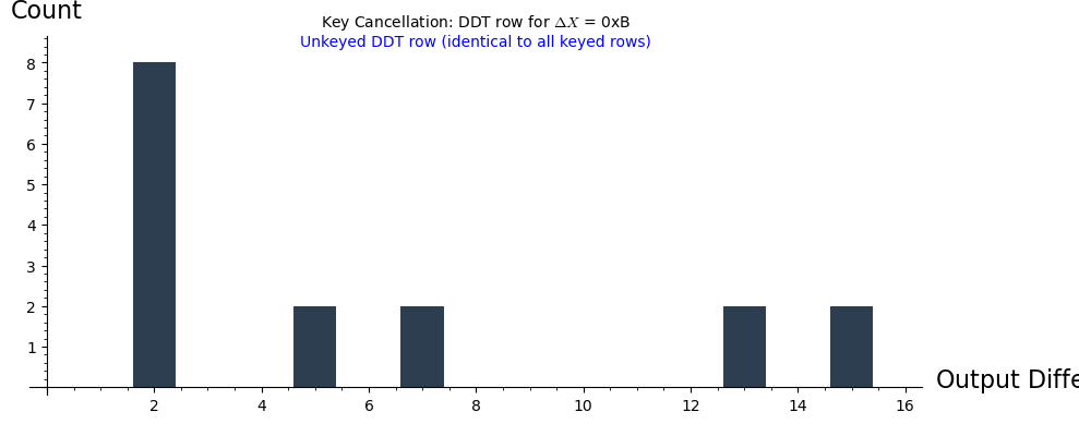
Unkeyed row:  [0, 0, 8, 0, 0, 2, 0, 2, 0, 0, 0, 0, 0, 2, 0, 2]
Keyed (K=7):  [0, 0, 8, 0, 0, 2, 0, 2, 0, 0, 0, 0, 0, 2, 0, 2]
Rows match: True
Observation
The key cancellation property is confirmed: all 16 possible keys produce exactly the same output difference distribution for a given input difference. The bars for all keys overlap perfectly. This is the fundamental reason why differential cryptanalysis works: the attacker can precompute the DDT of the unkeyed S-box and use it to predict the behavior of the keyed cipher.
Experiment 3: Comparing S-box Designs#
We compare the DDTs of three different S-box designs:
Heys tutorial S-box (educational, moderate resistance)
AES S-box (SubBytes, 8-bit, designed for near-optimal differential resistance)
Random permutation (baseline)
# --- Define the three S-boxes ---

# 1. Heys S-box (4-bit)
HEYS_SBOX = [0xE, 0x4, 0xD, 0x1, 0x2, 0xF, 0xB, 0x8,
             0x3, 0xA, 0x6, 0xC, 0x5, 0x9, 0x0, 0x7]

# 2. AES S-box (8-bit) -- full 256-entry SubBytes table
AES_SBOX = [
    0x63, 0x7C, 0x77, 0x7B, 0xF2, 0x6B, 0x6F, 0xC5,
    0x30, 0x01, 0x67, 0x2B, 0xFE, 0xD7, 0xAB, 0x76,
    0xCA, 0x82, 0xC9, 0x7D, 0xFA, 0x59, 0x47, 0xF0,
    0xAD, 0xD4, 0xA2, 0xAF, 0x9C, 0xA4, 0x72, 0xC0,
    0xB7, 0xFD, 0x93, 0x26, 0x36, 0x3F, 0xF7, 0xCC,
    0x34, 0xA5, 0xE5, 0xF1, 0x71, 0xD8, 0x31, 0x15,
    0x04, 0xC7, 0x23, 0xC3, 0x18, 0x96, 0x05, 0x9A,
    0x07, 0x12, 0x80, 0xE2, 0xEB, 0x27, 0xB2, 0x75,
    0x09, 0x83, 0x2C, 0x1A, 0x1B, 0x6E, 0x5A, 0xA0,
    0x52, 0x3B, 0xD6, 0xB3, 0x29, 0xE3, 0x2F, 0x84,
    0x53, 0xD1, 0x00, 0xED, 0x20, 0xFC, 0xB1, 0x5B,
    0x6A, 0xCB, 0xBE, 0x39, 0x4A, 0x4C, 0x58, 0xCF,
    0xD0, 0xEF, 0xAA, 0xFB, 0x43, 0x4D, 0x33, 0x85,
    0x45, 0xF9, 0x02, 0x7F, 0x50, 0x3C, 0x9F, 0xA8,
    0x51, 0xA3, 0x40, 0x8F, 0x92, 0x9D, 0x38, 0xF5,
    0xBC, 0xB6, 0xDA, 0x21, 0x10, 0xFF, 0xF3, 0xD2,
    0xCD, 0x0C, 0x13, 0xEC, 0x5F, 0x97, 0x44, 0x17,
    0xC4, 0xA7, 0x7E, 0x3D, 0x64, 0x5D, 0x19, 0x73,
    0x60, 0x81, 0x4F, 0xDC, 0x22, 0x2A, 0x90, 0x88,
    0x46, 0xEE, 0xB8, 0x14, 0xDE, 0x5E, 0x0B, 0xDB,
    0xE0, 0x32, 0x3A, 0x0A, 0x49, 0x06, 0x24, 0x5C,
    0xC2, 0xD3, 0xAC, 0x62, 0x91, 0x95, 0xE4, 0x79,
    0xE7, 0xC8, 0x37, 0x6D, 0x8D, 0xD5, 0x4E, 0xA9,
    0x6C, 0x56, 0xF4, 0xEA, 0x65, 0x7A, 0xAE, 0x08,
    0xBA, 0x78, 0x25, 0x2E, 0x1C, 0xA6, 0xB4, 0xC6,
    0xE8, 0xDD, 0x74, 0x1F, 0x4B, 0xBD, 0x8B, 0x8A,
    0x70, 0x3E, 0xB5, 0x66, 0x48, 0x03, 0xF6, 0x0E,
    0x61, 0x35, 0x57, 0xB9, 0x86, 0xC1, 0x1D, 0x9E,
    0xE1, 0xF8, 0x98, 0x11, 0x69, 0xD9, 0x8E, 0x94,
    0x9B, 0x1E, 0x87, 0xE9, 0xCE, 0x55, 0x28, 0xDF,
    0x8C, 0xA1, 0x89, 0x0D, 0xBF, 0xE6, 0x42, 0x68,
    0x41, 0x99, 0x2D, 0x0F, 0xB0, 0x54, 0xBB, 0x16,
]

# 3. Random 4-bit permutation (for comparison with Heys)
set_random_seed(42)
RANDOM_SBOX_4 = Permutations(16).random_element()
RANDOM_SBOX_4 = [x - 1 for x in RANDOM_SBOX_4]  # 0-indexed

print('S-box definitions:')
print(f'  Heys:   {[hex(x) for x in HEYS_SBOX]}')
print(f'  AES:    [{hex(AES_SBOX[0])}, {hex(AES_SBOX[1])}, ..., '
      f'{hex(AES_SBOX[254])}, {hex(AES_SBOX[255])}] (256 entries)')
print(f'  Random: {[hex(x) for x in RANDOM_SBOX_4]}')
S-box definitions:
  Heys:   ['0xe', '0x4', '0xd', '0x1', '0x2', '0xf', '0xb', '0x8', '0x3', '0xa', '0x6', '0xc', '0x5', '0x9', '0x0', '0x7']
  AES:    [0x63, 0x7c, ..., 0xbb, 0x16] (256 entries)
  Random: ['0xb', '0x2', '0x3', '0xc', '0x6', '0xd', '0x5', '0x1', '0xf', '0x8', '0x0', '0xe', '0x7', '0xa', '0x4', '0x9']
def compute_ddt_sage(sbox):
    """Compute the DDT as a SageMath matrix for any S-box (given as a list)."""
    n_in = len(sbox)
    n_out = max(sbox) + 1
    ddt = [[0] * n_out for _ in range(n_in)]
    for delta_in in range(n_in):
        for x in range(n_in):
            x_prime = x ^^ delta_in
            delta_out = int(sbox[x]) ^^ int(sbox[x_prime])
            ddt[delta_in][delta_out] += 1
    return matrix(ZZ, ddt)

def differential_uniformity(ddt_mat):
    """Max DDT entry excluding the trivial (0,0) entry."""
    best = 0
    for i in range(ddt_mat.nrows()):
        for j in range(ddt_mat.ncols()):
            if i == 0 and j == 0:
                continue
            if ddt_mat[i, j] > best:
                best = ddt_mat[i, j]
    return best

def max_dp(ddt_mat):
    """Maximum differential probability (excluding 0->0)."""
    return differential_uniformity(ddt_mat) / ddt_mat.nrows()

# Compute DDTs
ddt_heys = compute_ddt_sage(HEYS_SBOX)
ddt_rand = compute_ddt_sage(RANDOM_SBOX_4)

# Side-by-side matrix_plot comparison
p1 = matrix_plot(ddt_heys, cmap='YlOrRd', colorbar=True)
p2 = matrix_plot(ddt_rand, cmap='YlOrRd', colorbar=True)

show(p1, figsize=6, title=f'Heys S-box (max dp = {float(max_dp(ddt_heys)):.3f})')
show(p2, figsize=6, title=f'Random Permutation (max dp = {float(max_dp(ddt_rand)):.3f})')

print(f'Heys S-box:  differential uniformity = {differential_uniformity(ddt_heys)}, '
      f'max dp = {float(max_dp(ddt_heys)):.4f}')
print(f'Random perm: differential uniformity = {differential_uniformity(ddt_rand)}, '
      f'max dp = {float(max_dp(ddt_rand)):.4f}')
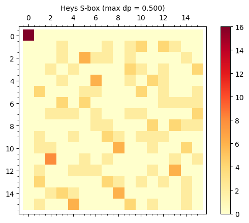
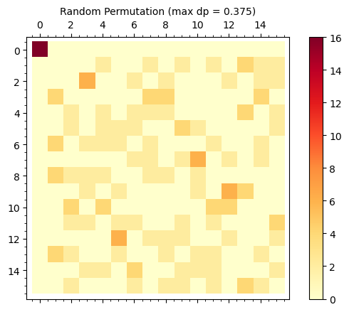
Heys S-box:  differential uniformity = 8, max dp = 0.5000
Random perm: differential uniformity = 6, max dp = 0.3750
# AES S-box DDT (8-bit: 256x256 table)
ddt_aes = compute_ddt_sage(AES_SBOX)
print(f'AES S-box: {len(AES_SBOX)} inputs, {max(AES_SBOX)+1} outputs')
print(f'DDT shape: {ddt_aes.nrows()} x {ddt_aes.ncols()}')
print(f'Differential uniformity: {differential_uniformity(ddt_aes)}')
print(f'Max dp (excl. 0->0): {float(max_dp(ddt_aes)):.6f}')
print(f'Ideal dp for random 8-bit function: {float(1/256):.6f}')
print(f'Ratio to ideal: {float(max_dp(ddt_aes) / (1/256)):.1f}x')
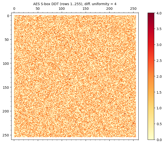
# Visualize AES DDT as matrix_plot (exclude row 0 for better contrast)
ddt_aes_display = ddt_aes[1:, :]
p_aes = matrix_plot(ddt_aes_display, cmap='YlOrRd', colorbar=True)
show(p_aes, figsize=8,
title=f'AES S-box DDT (rows 1..255), diff. uniformity = {differential_uniformity(ddt_aes)}')
# Entry value distribution
from collections import Counter
nonzero_entries = [ddt_aes[i, j] for i in range(1, 256) for j in range(256)]
counts = Counter(nonzero_entries)
total = len(nonzero_entries)
print(f'\nDDT entry value distribution (rows 1..255):')
for val in sorted(counts.keys()):
print(f' Value {val}: appears {counts[val]} times ({float(counts[val])/total*100:.1f}%)')
AES S-box: 256 inputs, 256 outputs
DDT shape: 256 x 256
Differential uniformity: 4
Max dp (excl. 0->0): 0.015625
Ideal dp for random 8-bit function: 0.003906
Ratio to ideal: 4.0x
DDT entry value distribution (rows 1..255):
  Value 0: appears 32895 times (50.4%)
  Value 2: appears 32130 times (49.2%)
  Value 4: appears 255 times (0.4%)
Observation
The AES S-box achieves the theoretical minimum differential uniformity of 4 for an 8-bit S-box (it is an almost perfect nonlinear or APN-like function). This means the maximum differential probability is \(4/256 = 1/64 \approx 0.0156\), only 4 times the ideal bound of \(1/256\). By contrast, the Heys 4-bit S-box has differential uniformity 6, giving max dp \(= 6/16 = 0.375\), which is 6 times the ideal \(1/16\). The AES S-box is specifically constructed via the multiplicative inverse in \(\text{GF}(2^8)\) to achieve this near-optimal resistance.
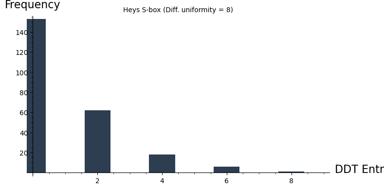
Experiment 4: Distribution of Differential Probabilities#
We compare the histogram of DDT entry values across different S-box designs. An ideal S-box would have all non-trivial DDT entries as small and uniform as possible.
# Distribution of DDT entry values for Heys S-box
entries_heys = [ddt_heys[i, j] for i in range(1, 16) for j in range(16)]
entries_rand = [ddt_rand[i, j] for i in range(1, 16) for j in range(16)]
from collections import Counter
hist_heys = Counter(entries_heys)
hist_rand = Counter(entries_rand)
max_val = max(max(hist_heys.keys()), max(hist_rand.keys()))
heys_data = [hist_heys.get(v, 0) for v in range(max_val + 1)]
rand_data = [hist_rand.get(v, 0) for v in range(max_val + 1)]
p1 = bar_chart(heys_data, color='#2c3e50', width=0.8)
show(p1, figsize=(8, 4), axes_labels=['DDT Entry Value', 'Frequency'],
title=f'Heys S-box (Diff. uniformity = {differential_uniformity(ddt_heys)})')
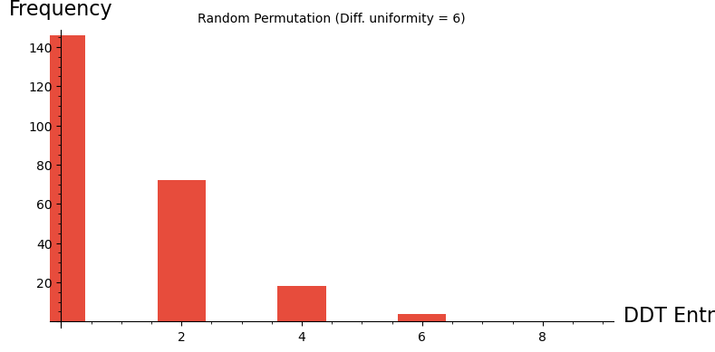
p2 = bar_chart(rand_data, color='#e74c3c', width=0.8)
show(p2, figsize=(8, 4), axes_labels=['DDT Entry Value', 'Frequency'],
title=f'Random Permutation (Diff. uniformity = {differential_uniformity(ddt_rand)})')
# Compare Heys S-box against 200 random 4-bit permutations
n_random = 200
random_max_dps = []
random_uniformities = []

for seed in range(n_random):
    set_random_seed(seed + 1000)
    rand_sbox = Permutations(16).random_element()
    rand_sbox = [x - 1 for x in rand_sbox]  # 0-indexed
    ddt_i = compute_ddt_sage(rand_sbox)
    random_max_dps.append(float(max_dp(ddt_i)))
    random_uniformities.append(differential_uniformity(ddt_i))

# Histogram of max dp values
from collections import Counter
dp_hist = Counter([round(x, 3) for x in random_max_dps])
dp_values = sorted(dp_hist.keys())
dp_counts = [dp_hist[v] for v in dp_values]

p3 = bar_chart(dp_counts, color='#3498db', width=0.8)
show(p3, figsize=(8, 4), axes_labels=['Bin index', 'Count (of 200 S-boxes)'],
     title='Max dp of 200 Random 4-bit Permutations')

heys_max_dp = float(max_dp(ddt_heys))
mean_random_dp = sum(random_max_dps) / len(random_max_dps)
std_random_dp = (sum((x - mean_random_dp)^2 for x in random_max_dps) / len(random_max_dps))^0.5

print(f'Statistics over {n_random} random 4-bit permutations:')
print(f'  Mean max dp: {float(mean_random_dp):.4f}')
print(f'  Std  max dp: {float(std_random_dp):.4f}')
print(f'  Min  max dp: {float(min(random_max_dps)):.4f}')
print(f'  Max  max dp: {float(max(random_max_dps)):.4f}')
print(f'  Heys max dp: {float(heys_max_dp):.4f}')
pct = sum(1 for x in random_max_dps if x >= heys_max_dp) / len(random_max_dps) * 100
print(f'\nHeys S-box percentile among random: {float(pct):.0f}%')
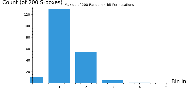
Statistics over 200 random 4-bit permutations:
  Mean max dp: 0.4100
  Std  max dp: 0.0782
  Min  max dp: 0.2500
  Max  max dp: 0.7500
  Heys max dp: 0.5000

Heys S-box percentile among random: 30%
Observation
The DDT entry histograms reveal the differential profile of each S-box. For the Heys S-box, most entries are 0 or 2, with occasional entries of 4 or 6. The random permutation shows a similar pattern, though its differential uniformity can vary. Comparing the Heys S-box against 200 random permutations shows that its max dp is typical of a random 4-bit permutation – at this small size, there is limited room for optimization. The real gains from careful S-box design appear at larger sizes (8 bits, as in AES), where the gap between optimal and random constructions is much larger.
Experiment 5: Constructing Differential Characteristics#
After gathering the differential data for the S-boxes in a Substitution-Permutation Network (SPN), we possess the necessary information to identify a valuable differential characteristic for the entire cipher. This can be achieved by linking suitable difference pairs of S-boxes. By creating a differential characteristic involving specific S-box difference pairs in each round, which includes plaintext bits and data bits inputted into the final round of S-boxes, we can potentially compromise the cipher by recovering a portion of the subkey bits after the last round. An example is provided to demonstrate the establishment of a differential characteristic.
Read paragraph \(\S 4.3\) of Heys about the combination of differential characteristics in three rounds of SPN to find a differential characteristic that will be used to attack the cipher.
def SPNEncryptionL(plaintext16, key28):
    expkey=KeySchedule(key28)
    state=plaintext16

    #round 1
    state=ListXOR(state,RoundKey(expkey,0))
    state=S(state)
    state=P(state)

    #round 2

    state=ListXOR(state,RoundKey(expkey,1))
    state=S(state)
    state=P(state)

    #round 3
    leak = state
    state=ListXOR(state,RoundKey(expkey,2))
    state=S(state)

    #final XOR
    state=ListXOR(state,RoundKey(expkey,3))

    return state, leak
#This is our differential characteristic. Read the paragraph 4.3 from heys.pdf to understand this choice.
deltaU3=[0,0,0,0,0,0,1,0,0,0,1,0,0,0,0,0]
deltaP =[0,0,0,0,1,0,1,1,0,0,0,0,0,0,0,0]
key=[choice([0,1])]*28#[0,1]*14
c=0
N=16
for i in range(2^N):
    digs=(ZZ(i)).digits(2)
    digs.extend([0] * (16-len(digs)))
    _,u1=SPNEncryptionL(ListXOR(digs,deltaP),key)
    _,u2=SPNEncryptionL(ListXOR(digs,[0]*16),key)
    if not (ListXOR(u1,u2)==deltaU3):
        c+=1
c/2.0^N #probability of success
0.812500000000000
1-3/16.0 #confirm with 4.3 from heys.pdf
0.812500000000000
c1,u1=SPNEncryptionL(ListXOR([1]*16,deltaP),[0,1]*14)
c2,u2=SPNEncryptionL(ListXOR([1]*16,[0]*16),[0,1]*14)
ListXOR(u1,u2)==deltaU3
True
Preparing the attack#
For a given key we prepare 1024 pairs of plaintext-ciphertext which (in pairs) differ by the differential \(\Delta P\). This is then used to cryptanalyze the chosen key. We recover from our differential characteristic the parts of the key indicated by \(k_1\) and \(k_2\).
#key=[0,1]*14
k1=HexToBlock('A')
k2=HexToBlock('C')
key=[choice([0,1])]*16+k1+k2+[choice([0,1])]*4
c=0
N=9
cpli=[]
for i in range(2^N):
    digs=(ZZ(choice(range(2^16)))).digits(2)
    digs.extend([0] * (16-len(digs)))
    c1,u1=SPNEncryptionL(ListXOR(digs,deltaP),key)
    c2,u2=SPNEncryptionL(ListXOR(digs,[0]*16),key)
    cpli.append([[digs,c2],[ListXOR(digs,deltaP),c1]])
This is an enhanced encryption procedure which is used with the plaintext-ciphertext pairs to cryptanalyze the key.
def SPNEncryptionCompare(plaintext16,ciphertext16, key28):
    expkey=KeySchedule(key28)
    state=plaintext16

    #round 1
    state=ListXOR(state,RoundKey(expkey,0))
    state=S(state)
    state=P(state)

    #round 2

    state=ListXOR(state,RoundKey(expkey,1))
    state=S(state)
    state=P(state)

    #round 3
    leak = state
    #state=ListXOR(state,RoundKey(expkey,2))

    #state=S(state)
    #final XOR
    #state=ListXOR(state,RoundKey(expkey,3))

    #backtracking
    cstate=ListXOR(ciphertext16,RoundKey(expkey,3))
    cstate=Sinv(cstate)
    cstate=ListXOR(cstate,RoundKey(expkey,2))

    return leak, cstate
The following matching procedure computes how likely the given subkey is in relation to the fixed differential characteristic.
def Match(li,h1,h2):
    cou1=0
    cou2=0
    for i in range(len(li)):
        plain0=li[i][0][0]
        cipher0=li[i][0][1]
        plain1=li[i][1][0]
        cipher1=li[i][1][1]
        k1=HexToBlock(h1)
        k2=HexToBlock(h2)
        key=[0]*16+k1+k2+[0]*4 #dummy key filler
        l0,c0=SPNEncryptionCompare(plain0,cipher0,key)
        l1,c1=SPNEncryptionCompare(plain1,cipher1,key)
        if ListXOR(l0,l1)==deltaU3:
            cou1+=1
        if ListXOR(c0,c1)[4:13]==deltaU3[4:13]:
            cou2+=1
    return [cou1,cou2]
Differential cryptanalysis of the SPN#
Finally we perform a successful cryptanalysis of the SPN network designed above. We can read from the values in the table that by far the most likely choice of the subkey is the one which corresponds to the original fixed value. The remaining 20 bits of the key are recovered in a brute force computation.
N=len(cpli)
for h1 in vals:
    print(h1)
    print(sorted([[float(Match(cpli,h1,h2)[1])/N,h2] for h2 in vals]))
0
[[0.0, '6'], [0.0, '9'], [0.0, 'C'], [0.001953125, '1'], [0.001953125, '3'], [0.001953125, '5'], [0.001953125, '7'], [0.001953125, 'A'], [0.001953125, 'B'], [0.001953125, 'D'], [0.001953125, 'F'], [0.00390625, '0'], [0.00390625, '2'], [0.00390625, '4'], [0.005859375, '8'], [0.005859375, 'E']]
1
[[0.0, '0'], [0.0, '1'], [0.0, '2'], [0.0, '4'], [0.0, '5'], [0.0, '6'], [0.0, '7'], [0.0, '9'], [0.0, 'C'], [0.001953125, '3'], [0.001953125, 'A'], [0.001953125, 'B'], [0.001953125, 'F'], [0.00390625, 'D'], [0.005859375, '8'], [0.005859375, 'E']]
2
[[0.0, '1'], [0.0, '2'], [0.0, '6'], [0.0, '7'], [0.0, '9'], [0.0, 'C'], [0.001953125, '0'], [0.001953125, '4'], [0.001953125, '5'], [0.001953125, 'A'], [0.001953125, 'B'], [0.001953125, 'F'], [0.00390625, '3'], [0.00390625, 'D'], [0.005859375, '8'], [0.005859375, 'E']]
3
[[0.0, '0'], [0.0, '1'], [0.0, '6'], [0.0, '7'], [0.001953125, '3'], [0.001953125, '4'], [0.001953125, 'A'], [0.00390625, '9'], [0.00390625, 'D'], [0.005859375, '5'], [0.005859375, '8'], [0.005859375, 'B'], [0.005859375, 'E'], [0.005859375, 'F'], [0.01171875, '2'], [0.03125, 'C']]
4
[[0.0, '1'], [0.0, '4'], [0.0, '5'], [0.0, '6'], [0.0, '7'], [0.001953125, '9'], [0.00390625, '0'], [0.00390625, '3'], [0.00390625, 'D'], [0.005859375, '2'], [0.0078125, 'B'], [0.0078125, 'F'], [0.009765625, 'A'], [0.009765625, 'E'], [0.01171875, '8'], [0.0234375, 'C']]
5
[[0.0, '1'], [0.0, '5'], [0.0, '6'], [0.0, '7'], [0.0, '9'], [0.0, 'C'], [0.001953125, '0'], [0.001953125, '2'], [0.001953125, 'A'], [0.001953125, 'B'], [0.00390625, '3'], [0.00390625, 'D'], [0.00390625, 'F'], [0.005859375, '4'], [0.005859375, 'E'], [0.0078125, '8']]
6
[[0.0, '6'], [0.0, '8'], [0.0, '9'], [0.0, 'A'], [0.0, 'B'], [0.0, 'C'], [0.0, 'E'], [0.0, 'F'], [0.001953125, '1'], [0.001953125, '5'], [0.001953125, '7'], [0.001953125, 'D'], [0.005859375, '0'], [0.005859375, '2'], [0.005859375, '3'], [0.005859375, '4']]
7
[[0.0, '0'], [0.0, '1'], [0.0, '2'], [0.0, '3'], [0.0, '4'], [0.0, '5'], [0.0, '6'], [0.0, '7'], [0.0, '9'], [0.0, 'C'], [0.001953125, 'A'], [0.001953125, 'B'], [0.001953125, 'D'], [0.001953125, 'F'], [0.005859375, '8'], [0.005859375, 'E']]
8
[[0.0, '4'], [0.0, '6'], [0.0, '7'], [0.001953125, '0'], [0.001953125, '1'], [0.001953125, '3'], [0.001953125, '5'], [0.00390625, '2'], [0.0078125, 'D'], [0.009765625, '8'], [0.009765625, 'A'], [0.009765625, 'F'], [0.015625, '9'], [0.015625, 'E'], [0.017578125, 'B'], [0.0234375, 'C']]
9
[[0.0, '1'], [0.0, '4'], [0.0, '7'], [0.001953125, '0'], [0.001953125, '3'], [0.001953125, '6'], [0.005859375, '2'], [0.005859375, '5'], [0.013671875, 'D'], [0.015625, '8'], [0.015625, 'E'], [0.017578125, 'B'], [0.01953125, 'F'], [0.021484375, '9'], [0.021484375, 'A'], [0.044921875, 'C']]
A
[[0.001953125, '0'], [0.001953125, '4'], [0.001953125, '6'], [0.001953125, '7'], [0.00390625, '1'], [0.00390625, '3'], [0.01953125, '5'], [0.033203125, '2'], [0.037109375, '8'], [0.037109375, 'D'], [0.0390625, 'E'], [0.044921875, 'F'], [0.048828125, 'B'], [0.05078125, '9'], [0.052734375, 'A'], [0.15625, 'C']]
B
[[0.0, '0'], [0.0, '3'], [0.0, '4'], [0.0, '6'], [0.0, '7'], [0.001953125, '1'], [0.001953125, '2'], [0.00390625, '5'], [0.01171875, 'F'], [0.015625, 'D'], [0.017578125, '8'], [0.017578125, 'A'], [0.017578125, 'E'], [0.01953125, 'B'], [0.021484375, '9'], [0.03515625, 'C']]
C
[[0.001953125, '0'], [0.001953125, '1'], [0.001953125, '4'], [0.001953125, '6'], [0.001953125, '7'], [0.005859375, '3'], [0.005859375, '5'], [0.0078125, '2'], [0.013671875, 'E'], [0.017578125, '8'], [0.017578125, 'D'], [0.01953125, 'B'], [0.01953125, 'F'], [0.0234375, '9'], [0.02734375, 'A'], [0.0546875, 'C']]
D
[[0.0, '4'], [0.0, '6'], [0.0, '7'], [0.001953125, '1'], [0.00390625, '0'], [0.005859375, '3'], [0.0078125, '5'], [0.0078125, 'D'], [0.009765625, '2'], [0.009765625, '8'], [0.013671875, 'A'], [0.015625, 'F'], [0.017578125, '9'], [0.017578125, 'E'], [0.01953125, 'B'], [0.041015625, 'C']]
E
[[0.0, '0'], [0.0, '4'], [0.0, '7'], [0.001953125, '1'], [0.001953125, '2'], [0.001953125, '3'], [0.001953125, '6'], [0.005859375, '5'], [0.013671875, 'F'], [0.015625, 'D'], [0.017578125, 'A'], [0.017578125, 'E'], [0.01953125, '8'], [0.021484375, '9'], [0.021484375, 'B'], [0.03515625, 'C']]
F
[[0.0, '4'], [0.0, '6'], [0.0, '7'], [0.001953125, '0'], [0.001953125, '1'], [0.001953125, '3'], [0.00390625, '2'], [0.00390625, '5'], [0.015625, '8'], [0.015625, 'D'], [0.015625, 'F'], [0.021484375, 'A'], [0.021484375, 'E'], [0.0234375, 'B'], [0.025390625, '9'], [0.04296875, 'C']]
19.5 Exercises#
Exercise 19.1 (Warm-up)#
For the Heys S-box, manually verify the DDT entry for \(\Delta X = 5\), \(\Delta Y = 9\). List all inputs \(X\) such that \(S(X) \oplus S(X \oplus 5) = 9\).
Hint
Iterate over all \(X \in \{0, 1, \ldots, 15\}\), compute \(X' = X \oplus 5\), then
check whether \(S(X) \oplus S(X') = 9\). Remember that the S-box is
[0xE, 0x4, 0xD, 0x1, 0x2, 0xF, 0xB, 0x8, 0x3, 0xA, 0x6, 0xC, 0x5, 0x9, 0x0, 0x7].
The count should match DDT[5][9].
Exercise 19.2 (Applied)#
Write a function that, given an S-box, determines whether it is a bijection (permutation) by checking both the standard definition (all outputs distinct) and the DDT structure (column sums all equal \(2^n\)). Verify your function on the Heys S-box and on the non-bijective mapping \(S(x) = x \mathbin{\&} \texttt{0x7}\) (bitwise AND masking the top bit).
Hint
For the bijection check: len(set(sbox)) == len(sbox). For the DDT check:
compute the DDT using compute_ddt_sage() and verify that all column sums equal \(2^n\).
Use matrix(ZZ, ddt).transpose() to access column sums easily.
Exercise 19.3 (Analysis)#
Prove that all entries in the DDT of any S-box are even. More precisely, show that the solutions to \(S(X) \oplus S(X \oplus \Delta X) = \Delta Y\) always come in pairs.
Hint
If \(X_0\) is a solution (i.e., \(S(X_0) \oplus S(X_0 \oplus \Delta X) = \Delta Y\)), then \(X_0' = X_0 \oplus \Delta X\) is also a solution: \(S(X_0') \oplus S(X_0' \oplus \Delta X) = S(X_0 \oplus \Delta X) \oplus S(X_0) = \Delta Y\). If \(\Delta X \neq 0\), then \(X_0 \neq X_0'\), so solutions come in distinct pairs.
Exercise 19.4 (Theory)#
An S-box \(S: \{0,1\}^n \to \{0,1\}^n\) is called almost perfect nonlinear (APN) if its differential uniformity is exactly 2 (the minimum possible for \(n > 1\)). Show that the AES S-box is not APN (its differential uniformity is 4). Explain why no 8-bit bijective S-box can be APN.
Hint
Compute the AES DDT using compute_ddt_sage(AES_SBOX) and find the maximum entry.
For the impossibility result: it has been proven that APN permutations of
\(\{0,1\}^n\) exist only for odd \(n\). Since \(n = 8\) is even, no APN bijection
on 8 bits exists. The best achievable differential uniformity for an 8-bit
bijection is 4, which the AES S-box achieves.
Exercise 19.5 (Challenge)#
Search for the optimal 4-bit S-box: a permutation of \(\{0, \ldots, 15\}\) that minimizes the differential uniformity. Use a random search (generate 10,000 random permutations) and report:
The minimum differential uniformity found
How many of the 10,000 permutations achieve this minimum
A histogram of differential uniformities across all 10,000 permutations
Hint
For a 4-bit bijection, the minimum possible differential uniformity is 4
(since all DDT entries are even and each nonzero row sums to 16, there must
be at least one entry \(\geq 4\) when entries are distributed among 16 columns
with sum 16 and all entries even). Use Permutations(16).random_element()
to generate candidates and compute_ddt_sage() to evaluate each.
19.6 Summary#
Concept |
Key Point |
|---|---|
Differential cryptanalysis |
Study how XOR differences propagate through a cipher |
Input/output difference |
\(\Delta X = X \oplus X'\), \(\Delta Y = S(X) \oplus S(X')\) |
DDT |
\(2^n \times 2^m\) table counting how often each \(\Delta X\) produces each \(\Delta Y\) |
Differential probability |
\(\text{dp}(\Delta X \to \Delta Y) = \text{DDT}[\Delta X][\Delta Y] / 2^n\) |
Key cancellation |
XOR key mixing does not affect input differences |
DDT properties |
Row/column sums \(= 2^n\); all entries even; first row concentrated at 0 |
Differential uniformity |
Maximum DDT entry (excluding \(0 \to 0\)); lower is better |
AES S-box |
Differential uniformity 4 (optimal for 8-bit bijection) |
Historical significance |
NSA knew about differential cryptanalysis before DES was published |
Tip
The DDT is the fundamental data structure of differential cryptanalysis. In Chapter 20, we will use these differential probabilities to construct differential characteristics that trace a high-probability difference path through multiple rounds of a block cipher. In Chapter 21, we will mount a complete differential attack on a reduced-round SPN cipher, using the Heys S-box DDT computed in this chapter to recover secret key bits.
References#
Biham, E. and Shamir, A. (1991). “Differential Cryptanalysis of DES-like Cryptosystems.” Journal of Cryptology, 4(1), 3–72. The foundational paper that introduced differential cryptanalysis to the public cryptographic community. Presents the first attack on DES faster than brute force (\(2^{47}\) chosen plaintexts for the full 16 rounds). [9]
Heys, H. M. (2002). “A Tutorial on Linear and Differential Cryptanalysis.” Cryptologia, 26(3), 189–221. The standard pedagogical reference for both linear and differential cryptanalysis. The 4-bit S-box and SPN cipher used throughout this chapter and the next two chapters are from this tutorial. [11]
Coppersmith, D. (1994). “The Data Encryption Standard (DES) and its Strength Against Attacks.” IBM Journal of Research and Development, 38(3), 243–250. Reveals that the DES design team was aware of differential cryptanalysis (which they called the “T-attack”) and designed the S-boxes specifically to resist it. [12]
Nyberg, K. (1994). “Differentially Uniform Mappings for Cryptography.” EUROCRYPT ‘93, LNCS 765, 55–64. Formalizes the concept of differential uniformity and establishes the connection between S-box design and resistance to differential cryptanalysis. [13]
Daemen, J. and Rijmen, V. (2002). The Design of Rijndael: AES – The Advanced Encryption Standard. Springer. Describes the design rationale for the AES S-box, including its construction via multiplicative inversion in \(\text{GF}(2^8)\) to achieve optimal differential and linear properties. [14]
Biham, E. and Shamir, A. Differential Cryptanalysis of the Data Encryption Standard. Springer, 1993. Extended version with practical implementations of differential cryptanalytic attacks on many block ciphers.