
Chapter 8: The Playfair Cipher (SageMath)#
“There is nothing so practical as a good cipher that can be operated without any apparatus.” – Lord Playfair, advocating the cipher to the British Foreign Office, 1854
In the preceding chapters, we examined monoalphabetic and polyalphabetic ciphers that operate on individual letters. The Playfair cipher represents a fundamental shift in approach: it encrypts pairs of letters (digrams) simultaneously. This makes it the first widely used digraphic (or polygraphic) cipher in the history of military cryptography.
By operating on digrams rather than single letters, the Playfair cipher obscures the simple letter frequency distribution that makes monoalphabetic ciphers so vulnerable. However, as we shall see, it introduces a new kind of statistical regularity – digram frequency – that a skilled cryptanalyst can exploit.
Python Version Available
This notebook contains the SageMath implementation. A pure Python/NumPy version is available in Chapter 8: The Playfair Cipher.
8.1 Historical Context#
The Playfair cipher was invented in 1854 by Sir Charles Wheatstone (1802–1875), one of the most prolific British scientists and inventors of the Victorian era. Wheatstone is better known for his contributions to the electric telegraph and the Wheatstone bridge circuit, but his cryptographic work was equally innovative.
Despite being Wheatstone’s invention, the cipher bears the name of Baron Lyon Playfair (1818–1898), a Scottish chemist and politician who enthusiastically promoted the system to the British Foreign Office. Playfair demonstrated the cipher at a dinner party to Lord Palmerston (then Prime Minister) and other government officials. According to legend, Palmerston found the system too complex, to which Playfair responded by teaching it to three boys from a nearby school in fifteen minutes – proving its practicality.
Military adoption and legacy
The Playfair cipher saw remarkable longevity in military service:
Boer War (1899–1902): First large-scale military use by British forces in South Africa.
World War I (1914–1918): Used by British tactical communications when speed was more important than absolute security.
World War II (1939–1945): Used by Australian and New Zealand forces (ANZAC) for lower-level tactical messages, and by the British Special Operations Executive (SOE) for covert communications in occupied Europe.
The Playfair cipher was valued not for its theoretical strength – which was known to be limited – but for its operational convenience. It required no equipment, could be memorised by field agents, and was fast enough for real-time communication. It represented an excellent trade-off between security and usability for its era.
The Playfair cipher holds the distinction of being the first practical digraphic cipher in widespread military use. Its central innovation – encrypting letter pairs using a 5\(\times\)5 grid – influenced later polygraphic systems, including the Hill cipher (Chapter 7) and the ADFGVX cipher used by Germany in World War I.
8.2 Formal Definitions#
8.2.1 The Playfair Grid#
The Playfair cipher operates using a 5\(\times\)5 matrix (grid) containing 25 distinct letters of the English alphabet. Since the English alphabet has 26 letters but the grid has only 25 cells, the letters I and J are traditionally merged into a single cell (treated as the same letter).
Definition 8.1 (Playfair Grid)
A Playfair grid is a 5\(\times\)5 matrix \(G\) whose 25 entries are a permutation of the alphabet \(\mathcal{A} = \{A, B, C, D, E, F, G, H, I, K, L, M, N, O, P, Q, R, S, T, U, V, W, X, Y, Z\}\) (with I/J identified). Each letter appears exactly once.
The grid is constructed from a keyword \(\kappa\) as follows:
Convert \(\kappa\) to uppercase and replace every J with I.
Remove duplicate letters, keeping only the first occurrence of each.
Append the remaining unused letters of \(\mathcal{A}\) in alphabetical order.
Fill the 5\(\times\)5 matrix row by row with the resulting 25-letter sequence.
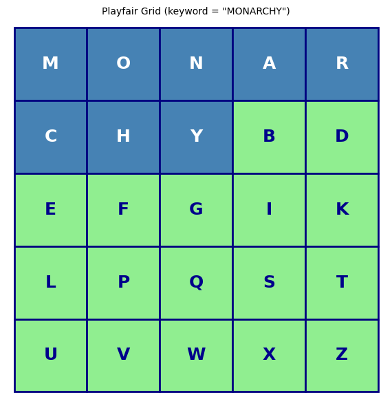
Example. For keyword MONARCHY, the grid construction proceeds as:
Keyword letters (deduplicated): M, O, N, A, R, C, H, Y
Remaining alphabet letters: B, D, E, F, G, I, K, L, P, Q, S, T, U, V, W, X, Z
Combined sequence: M O N A R C H Y B D E F G I K L P Q S T U V W X Z
8.2.2 Digram Preparation#
Before encryption, the plaintext must be prepared into a sequence of digrams (letter pairs).
Definition 8.2 (Digram Preparation)
Given a plaintext string \(m\):
Convert to uppercase and replace J with I.
Remove all non-alphabetic characters.
Split into consecutive pairs of letters.
If both letters in a pair are identical, insert an X between them and re-pair.
If the final group contains only one letter, pad it with X.
The result is a sequence of digrams \((d_1, d_2, \ldots, d_n)\) where each \(d_i = (a_i, b_i)\) with \(a_i \neq b_i\).
Example. BALLOON \(\to\) BA, LX, LO, ON (X inserted between the two L’s).
8.2.3 The Three Encryption Rules#
Given a digram \((a, b)\) with grid positions \((r_a, c_a)\) and \((r_b, c_b)\), the Playfair cipher applies one of three rules:
Definition 8.3 (Playfair Encryption Rules)
Rule 1 – Same Row: If \(r_a = r_b\) (both letters are in the same row), replace each letter by the letter immediately to its right in the grid, wrapping around:
Rule 2 – Same Column: If \(c_a = c_b\) (both letters are in the same column), replace each letter by the letter immediately below it in the grid, wrapping around:
Rule 3 – Rectangle: If neither row nor column matches, the two letters define the corners of a rectangle. Replace each letter by the letter in its own row but the other letter’s column:
Decryption reverses these rules: shift left for same-row, shift up for same-column, and the rectangle rule is its own inverse.
Vulnerability
The Playfair cipher is a fixed permutation on the space of \(25 \times 24 = 600\) ordered digrams (since \(a \neq b\) is enforced). While this is a much larger space than the 26-letter monoalphabetic substitution, it is still subject to digram frequency analysis. In English, certain digrams (TH, HE, IN, ER, AN, …) occur far more frequently than others, and this statistical fingerprint is preserved – just mapped to different digram pairs.
8.3 Implementation#
We now build a complete Playfair cipher implementation in SageMath. The code below is taken from the original course materials.
# Create a 5x5 matrix using a secret key
def create_matrix(key):
    key = key.upper()
    matrix = [[0 for i in range (5)] for j in range(5)]
    letters_added = []
    row = 0
    col = 0
    # add the key to the matrix
    for letter in key:
        if letter not in letters_added:
            matrix[row][col] = letter
            letters_added.append(letter)
        else:
            continue
        if (col==4):
            col = 0
            row += 1
        else:
            col += 1
    #Add the rest of the alphabet to the matrix
    # A=65 ... Z=90
    for letter in range(65,91):
        if letter==74: # I/J are in the same position
                continue
        if chr(letter) not in letters_added: # Do not add repeated letters
            letters_added.append(chr(letter))

    index = 0
    for i in range(5):
        for j in range(5):
            matrix[i][j] = letters_added[index]
            index+=1
    return matrix
#Add fillers if the same letter is in a pair
def separate_same_letters(message):
    index = 0
    while (index<len(message)):
        l1 = message[index]
        if index == len(message)-1:
            message = message + 'X'
            index += 2
            continue
        l2 = message[index+1]
        if l1==l2:
            message = message[:index+1] + "X" + message[index+1:]
        index +=2
    return message
#Return the index of a letter in the matrix
#This will be used to know what rule (1-4) to apply
def indexOf(letter,matrix):
    for i in range (5):
        try:
            index = matrix[i].index(letter)
            return (i,index)
        except:
            continue

#Implementation of the playfair cipher
#If encrypt=True the method will encrypt the message
# otherwise the method will decrypt
def playfair(key, message, encrypt=True):
    inc = 1
    if encrypt==False:
        inc = -1
    matrix = create_matrix(key)
    message = message.upper()
    message = message.replace(' ','')
    message = separate_same_letters(message)
    cipher_text=''
    for (l1, l2) in zip(message[0::2], message[1::2]):
        row1,col1 = indexOf(l1,matrix)
        row2,col2 = indexOf(l2,matrix)
        if row1==row2: #Rule 2, the letters are in the same row
            cipher_text += matrix[row1][(col1+inc)%5] + matrix[row2][(col2+inc)%5]
        elif col1==col2:# Rule 3, the letters are in the same column
            cipher_text += matrix[(row1+inc)%5][col1] + matrix[(row2+inc)%5][col2]
        else: #Rule 4, the letters are in a different row and column
            cipher_text += matrix[row1][col2] + matrix[row2][col1]

    return cipher_text
# --- Demonstration ---
print('Playfair Grid (keyword = SECRET):')
m = create_matrix('SECRET')
for row in m:
    print(' '.join(row))

print()
print('Encrypting:')
ct = playfair('secret', 'my secret message')
print(f'  Plaintext:  MY SECRET MESSAGE')
print(f'  Ciphertext: {ct}')
print()
print('Decrypting:')
dt = playfair('secret', ct, False)
print(f'  Ciphertext: {ct}')
print(f'  Decrypted:  {dt}')
Playfair Grid (keyword = SECRET):
S E C R T
A B D F G
H I K L M
N O P Q U
V W X Y Z

Encrypting:
  Plaintext:  MY SECRET MESSAGE
  Ciphertext: LZECRTCSITCVAHBT

Decrypting:
  Ciphertext: LZECRTCSITCVAHBT
  Decrypted:  MYSECRETMESXSAGE
Implementation note
The separate_same_letters function handles three edge cases that arise in Playfair encryption:
Repeated letters: When two identical letters fall in the same digram (e.g., LL in BALLOON), an X is inserted between them to break the pair. This is necessary because the Playfair rules require the two letters in a digram to occupy different grid positions.
Odd-length text: If the cleaned text has an odd number of characters, a trailing X is appended to form the final digram.
I/J merging: Since the 5\(\times\)5 grid has only 25 cells, J is replaced by I throughout. This means the cipher cannot distinguish between I and J in the decrypted output.
Let us also demonstrate with the MONARCHY grid from the formal definitions:
print('Playfair Grid (keyword = MONARCHY):')
m = create_matrix('MONARCHY')
for row in m:
    print(' '.join(row))

print()
pt = 'INSTRUMENTS'
ct = playfair('MONARCHY', pt)
dt = playfair('MONARCHY', ct, False)
print(f'Plaintext:  {pt}')
print(f'Encrypted:  {ct}')
print(f'Decrypted:  {dt}')
Playfair Grid (keyword = MONARCHY):
M O N A R
C H Y B D
E F G I K
L P Q S T
U V W X Z

Plaintext:  INSTRUMENTS
Encrypted:  GATLMZCLRQXA
Decrypted:  INSTRUMENTSX
8.4 Cryptanalysis of the Playfair Cipher#
8.4.1 The Digram Permutation#
Theorem 8.1 (Playfair as a Digram Permutation)
For a fixed Playfair grid \(G\), the encryption function \(E_G\) is a permutation on the set of 600 ordered digrams \(\{(a, b) \in \mathcal{A}^2 : a \neq b\}\). That is, \(E_G\) is a bijection.
Proof sketch. Each of the three Playfair rules (same row, same column, rectangle) maps a digram \((a, b)\) to a unique digram \((a', b')\) with \(a' \neq b'\). The inverse rules (shift left, shift up, rectangle swap) provide an explicit inverse for each case. Since \(E_G\) is an invertible map on a finite set, it is a permutation. \(\square\)
8.4.2 Digram Frequency Analysis#
Because \(E_G\) is a fixed permutation on digrams, the frequency distribution of digrams is preserved (just relabelled). In English, certain digrams occur much more frequently than others:
Rank |
Digram |
Approx. Frequency |
|---|---|---|
1 |
TH |
3.56% |
2 |
HE |
3.07% |
3 |
IN |
2.43% |
4 |
ER |
2.05% |
5 |
AN |
1.99% |
6 |
RE |
1.85% |
7 |
ON |
1.76% |
8 |
AT |
1.49% |
9 |
EN |
1.45% |
10 |
ND |
1.35% |
An analyst who identifies the most frequent ciphertext digrams can attempt to match them against these expected English digram frequencies.
8.4.3 Hill-Climbing / Simulated Annealing Attack#
Modern computational attacks on the Playfair cipher use hill-climbing or simulated annealing with a fitness function based on quadgram statistics:
Start with a random 5\(\times\)5 grid.
Decrypt the ciphertext using this grid.
Score the resulting plaintext using log-probabilities of quadgrams (4-letter sequences).
Make a small random modification to the grid (swap two letters, swap two rows, swap two columns, etc.).
If the new grid produces a higher score, keep it; otherwise accept with probability \(e^{\Delta F / T}\) (simulated annealing).
Repeat until convergence.
This approach can break Playfair ciphers with as few as 100–200 characters of ciphertext.
Experiments#
Experiment 1: Visualising the Playfair Grid#
We display the 5\(\times\)5 Playfair grid using SageMath graphics, highlighting the keyword letters.
def visualise_playfair_grid_sage(keyword):
"""Display the Playfair grid as a coloured SageMath graphic."""
mat = create_matrix(keyword.upper())
kw = keyword.upper().replace('J', 'I')
kw_letters = set()
for c in kw:
if c.isalpha():
kw_letters.add(c)
G = Graphics()
for i in range(5):
for j in range(5):
letter = mat[i][j]
x, y = j, 4 - i
if letter in kw_letters:
color = 'steelblue'
txt_color = 'white'
else:
color = 'lightgreen'
txt_color = 'darkblue'
G += polygon2d([(x,y), (x+1,y), (x+1,y+1), (x,y+1)],
color=color, edgecolor='navy', thickness=2)
G += text(letter, (x+0.5, y+0.5), fontsize=18,
color=txt_color, fontweight='bold')
G.axes(False)
show(G, figsize=[6,6], title=f'Playfair Grid (keyword = "{keyword.upper()}")')
# Display grids for two different keywords
visualise_playfair_grid_sage('MONARCHY')
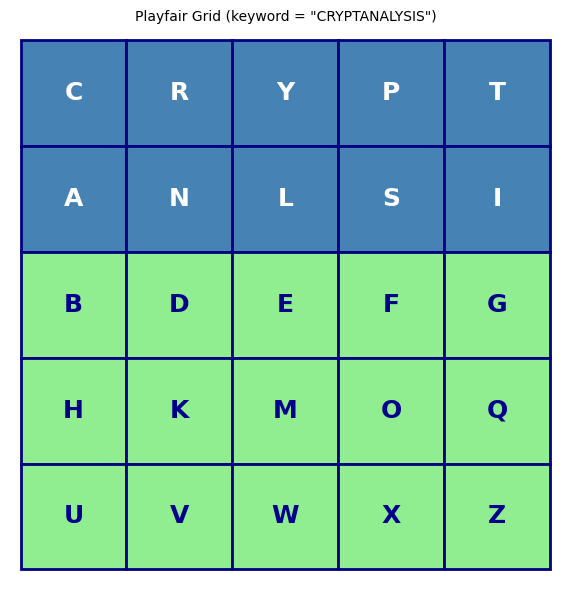
visualise_playfair_grid_sage('CRYPTANALYSIS')
Observation
The grid visualisation clearly shows how the keyword letters fill the first positions (blue cells) and the remaining alphabet letters follow in order (green cells). Different keywords produce completely different grids, and even a small change in the keyword rearranges many cells. The total number of possible Playfair grids is \(25! \approx 1.55 \times 10^{25}\), though many of these produce equivalent encryption due to row/column symmetries.
Experiment 2: Step-by-Step Encryption with Rule Annotations#
We encrypt a plaintext one digram at a time, showing which rule (same row, same column, or rectangle) is applied at each step.
def encrypt_step_by_step(key, plaintext):
    """Encrypt plaintext showing each digram transformation and the rule applied."""
    mat = create_matrix(key)
    message = plaintext.upper().replace(' ', '').replace('J', 'I')
    message = separate_same_letters(message)

    print(f'Plaintext:  {plaintext}')
    print(f'Prepared:   {" ".join([message[i:i+2] for i in range(0, len(message), 2)])}')
    print()
    print(f'{"Step":>4s}  {"Input":>6s}  {"Pos(a)":>8s}  {"Pos(b)":>8s}  {"Rule":>12s}  {"Output":>6s}')
    print('-' * 58)

    rule_counts = {'Same Row': 0, 'Same Column': 0, 'Rectangle': 0}
    ciphertext = ''

    for step, (l1, l2) in enumerate(zip(message[0::2], message[1::2]), 1):
        row1, col1 = indexOf(l1, mat)
        row2, col2 = indexOf(l2, mat)

        if row1 == row2:
            rule = 'Same Row'
            ea = mat[row1][(col1+1)%5]
            eb = mat[row2][(col2+1)%5]
        elif col1 == col2:
            rule = 'Same Column'
            ea = mat[(row1+1)%5][col1]
            eb = mat[(row2+1)%5][col2]
        else:
            rule = 'Rectangle'
            ea = mat[row1][col2]
            eb = mat[row2][col1]

        rule_counts[rule] += 1
        ciphertext += ea + eb
        print(f'{int(step):>4d}  {l1}{l2:>5s}  ({row1},{col1})     ({row2},{col2})     {rule:>12s}  {ea}{eb:>5s}')

    print(f'\nCiphertext: {ciphertext}')
    print(f'\nRule distribution:')
    total = sum(rule_counts.values())
    for rule, count in rule_counts.items():
        pct = 100*count/total if total > 0 else 0
        print(f'  {rule:>12s}: {int(count):>3d} / {total} ({float(pct):.1f}%)')

    return ciphertext, rule_counts

# Demonstrate with the MONARCHY grid
print('Grid:')
m = create_matrix('MONARCHY')
for row in m:
    print(' '.join(row))
print()

ct, rules = encrypt_step_by_step('MONARCHY', 'MEET ME AT THE FOUNTAIN')
Grid:
M O N A R
C H Y B D
E F G I K
L P Q S T
U V W X Z

Plaintext:  MEET ME AT THE FOUNTAIN
Prepared:   ME ET ME AT TH EF OU NT AI NX

Step   Input    Pos(a)    Pos(b)          Rule  Output
----------------------------------------------------------
   1  M    E  (0,0)     (2,0)      Same Column  C    L
   2  E    T  (2,0)     (3,4)        Rectangle  K    L
   3  M    E  (0,0)     (2,0)      Same Column  C    L
   4  A    T  (0,3)     (3,4)        Rectangle  R    S
   5  T    H  (3,4)     (1,1)        Rectangle  P    D
   6  E    F  (2,0)     (2,1)         Same Row  F    G
   7  O    U  (0,1)     (4,0)        Rectangle  M    V
   8  N    T  (0,2)     (3,4)        Rectangle  R    Q
   9  A    I  (0,3)     (2,3)      Same Column  B    S
  10  N    X  (0,2)     (4,3)        Rectangle  A    W

Ciphertext: CLKLCLRSPDFGMVRQBSAW

Rule distribution:
      Same Row:   1 / 10 (10.0%)
   Same Column:   3 / 10 (30.0%)
     Rectangle:   6 / 10 (60.0%)
Observation
The three rules are intuitive:
Same Row: Both letters slide one position to the right (wrapping from the last column back to the first).
Same Column: Both letters slide one position downward (wrapping from the bottom row back to the top).
Rectangle: The two letters define opposite corners of a rectangle; each is replaced by the letter in the other corner of its row.
The rectangle rule is the most common in practice (it applies whenever the two letters are in different rows and different columns), and it accounts for roughly 70–80% of digrams in typical text.
Experiment 3: Simple Frequency Analysis#
Failure
We check that single-letter frequency analysis on Playfair ciphertext produces a distribution completely different from natural English – the classical frequency attack fails.
import re
import string

# Remove all non-lower case elements of the standard latin alphabet
def lclear(text):
    return re.sub(r'[^a-z]', '', text.lower())

# Load a substantial English text
counter = 0
longtxt = ''
with open('../crypt_old_course/Course/Modules/week2/clean/Ulysses_4300-0.txt', encoding='utf8') as f:
    for line in f:
        longtxt += lclear(line.strip())
        counter += 1

print(f'Loaded {counter} lines, {len(longtxt)} characters of cleaned text.')
Loaded 170 lines, 10193 characters of cleaned text.
# Single-letter frequency comparison: plaintext vs Playfair ciphertext
sample = longtxt[:10000].replace('j', 'i')
ct_sample = playfair('secret', sample).lower()

def letter_freqs(text):
    """Compute letter frequencies as a dictionary."""
    counts = {}
    for c in text:
        if c.isalpha():
            counts[c] = counts.get(c, 0) + 1
    total = sum(counts.values())
    return {k: v/total for k, v in sorted(counts.items())}

pt_freqs = letter_freqs(sample)
ct_freqs = letter_freqs(ct_sample)

# Plot side by side using SageMath bar_chart
alpha = sorted(set(list(pt_freqs.keys()) + list(ct_freqs.keys())))
pt_vals = [pt_freqs.get(c, 0) for c in alpha]
ct_vals = [ct_freqs.get(c, 0) for c in alpha]

P1 = bar_chart(pt_vals, color='steelblue')
P2 = bar_chart(ct_vals, color='firebrick')

show(graphics_array([P1, P2]), figsize=[14, 4])
print('Left: plaintext letter frequencies | Right: Playfair ciphertext letter frequencies')
print('Notice how the ciphertext distribution is much flatter -- single-letter frequency analysis fails.')

Left: plaintext letter frequencies | Right: Playfair ciphertext letter frequencies
Notice how the ciphertext distribution is much flatter -- single-letter frequency analysis fails.
Experiment 4: Digram Frequency Preservation#
The Playfair cipher preserves the digram structure of the text. We compute digram frequencies for both plaintext and ciphertext to verify this.
def Digrams(text):
    """Compute digram frequencies and return sorted list."""
    digs=dict()
    for i in range(len(text)-1):
        d=text[i:i+2]
        if d in digs.keys():
            digs[d]+=1
        else:
            digs[d]=1

    tot=sum([digs[x] for x in digs.keys()])
    for k in digs.keys():
        digs[k]/=tot*1.0
    return digs, sorted([[digs[v],v] for v in digs.keys()])
# Top 10 digrams in the Playfair ciphertext
ss=playfair('secret', longtxt[:30000].replace('j','i'))
_,di=Digrams(ss.lower())
print('Top 10 ciphertext digrams:')
for freq, dg in list(reversed(di))[:10]:
    print(f'  {dg}: {float(freq):.4f}')
Top 10 ciphertext digrams:
  is: 0.0249
  sm: 0.0212
  si: 0.0140
  ho: 0.0110
  mc: 0.0103
  es: 0.0103
  sb: 0.0100
  hv: 0.0098
  cs: 0.0092
  pa: 0.0087
# Verify round-trip: encrypt then decrypt should recover original digram structure
_,lg=Digrams(playfair('secret',playfair('secret', longtxt[:100000].replace('j','i')),False).lower())
print('Top 10 digrams after encrypt->decrypt round trip:')
for freq, dg in list(reversed(lg))[:10]:
    print(f'  {dg}: {float(freq):.4f}')
Top 10 digrams after encrypt->decrypt round trip:
  he: 0.0463
  th: 0.0402
  in: 0.0226
  nd: 0.0179
  an: 0.0179
  ed: 0.0161
  er: 0.0159
  ng: 0.0152
  ea: 0.0133
  st: 0.0123
# Show how the ciphertext is structured as digram pairs
print('First 20 ciphertext digrams:')
[ss[2*i:2*i+2] for i in range(20)]
First 20 ciphertext digrams:
['ES',
 'GS',
 'RI',
 'XQ',
 'MQ',
 'KU',
 'GO',
 'DP',
 'UZ',
 'KY',
 'MK',
 'AB',
 'PS',
 'GH',
 'RB',
 'EQ',
 'UG',
 'IS',
 'ES',
 'BH']
Observation
The plaintext digram frequency distribution is preserved (just relabelled) in the ciphertext. The most frequent ciphertext digrams correspond to the most frequent English digrams (TH, HE, IN, ER, AN, …), merely mapped to different letter pairs.
Experiment 5: Digram Frequency Heatmaps – Plaintext vs. Ciphertext#
We compute the 25\(\times\)25 digram frequency matrix for both a plaintext and its Playfair-encrypted ciphertext, then visualise them as heatmaps using SageMath’s matrix_plot.
# A substantial English plaintext
english_text = (
    "Ciphers oh ciphers secrets they keep "
    "Locked away in code deep and discreet "
    "Symbols and numbers jumbled and mixed "
    "A message encoded ready to be fixed "
    "Through history they have been used to hide "
    "Plans of war love letters beside "
    "The Rosetta Stone a mystery solved "
    "A codebreakers work duly evolved "
    "From Caesar to Enigma through time they change "
    "Yet the essence remains mysterious and strange "
    "A puzzle to solve a game to play "
    "A message to decipher in every way "
    "Crack the code reveal the truth "
    "A challenge to minds sharp and astute "
    "For ciphers oh ciphers they hold the key "
    "To secrets untold waiting to be set free "
    "Deep within the caves so dark and cold "
    "The dwarves they sat and stories told "
    "Of treasure hoards and ancient lore "
    "And secrets kept for evermore "
    "But in their hands they held a tool "
    "A wondrous thing so sharp and cool "
    "A blade of steel that could carve letters "
    "And keep their secrets safe forever"
)

# Playfair alphabet (I/J merged, no J)
PF_ALPHA = 'ABCDEFGHIKLMNOPQRSTUVWXYZ'
PF_INDEX = {ch: idx for idx, ch in enumerate(PF_ALPHA)}

def digram_frequency_matrix(text):
    """Compute a 25x25 digram frequency matrix (I/J merged)."""
    cleaned = text.upper().replace('J', 'I')
    cleaned = ''.join(c for c in cleaned if c in PF_INDEX)
    mat = [[0.0]*25 for _ in range(25)]
    for k in range(len(cleaned) - 1):
        i = PF_INDEX[cleaned[k]]
        j = PF_INDEX[cleaned[k + 1]]
        mat[i][j] += 1
    total = sum(sum(row) for row in mat)
    if total > 0:
        for i in range(25):
            for j in range(25):
                mat[i][j] /= total
    return matrix(RR, mat)  # SageMath matrix over the reals

# Encrypt the text
ct = playfair('MONARCHY', english_text.upper().replace(' ', '').replace('J', 'I'))

# Compute digram frequency matrices
pt_mat = digram_frequency_matrix(english_text)
ct_mat = digram_frequency_matrix(ct)

# Plot side by side using SageMath's matrix_plot
P1 = matrix_plot(pt_mat, cmap='YlOrRd')
P2 = matrix_plot(ct_mat, cmap='YlOrRd')

show(graphics_array([P1, P2]), figsize=[14, 6])
print('Left: Plaintext digram frequencies | Right: Ciphertext digram frequencies')
print('The statistical structure is preserved -- merely relabelled by the Playfair permutation.')
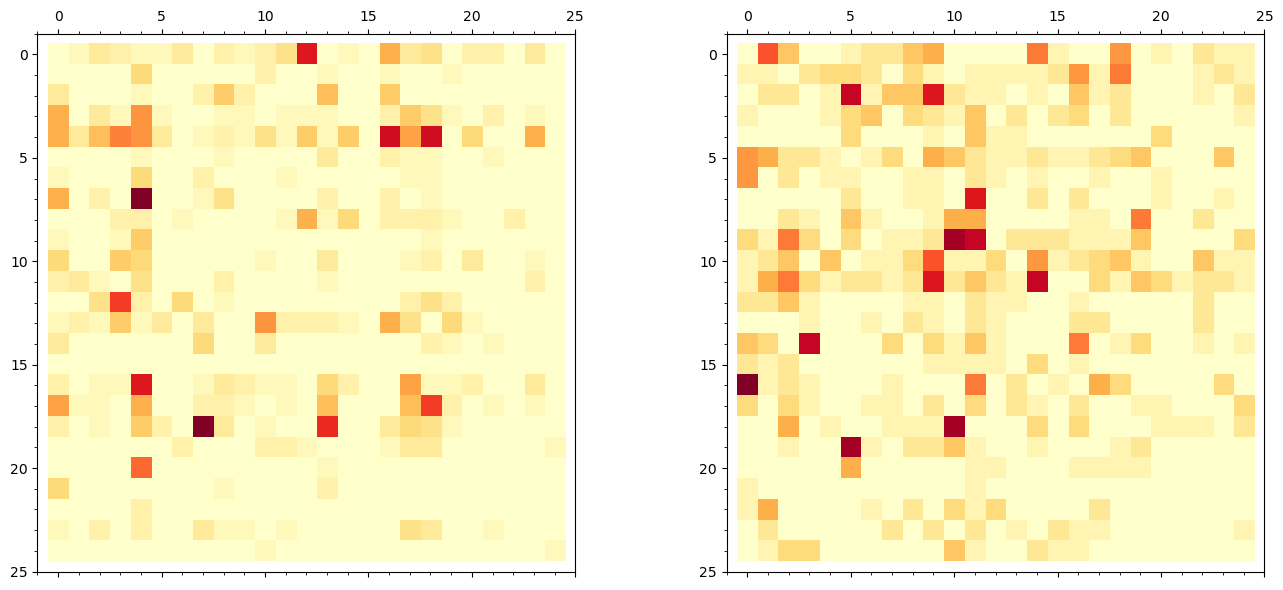
Left: Plaintext digram frequencies | Right: Ciphertext digram frequencies
The statistical structure is preserved -- merely relabelled by the Playfair permutation.
# Print the top digrams in each
def top_digrams(mat, n=10):
    flat = [(mat[i,j], PF_ALPHA[i]+PF_ALPHA[j]) for i in range(25) for j in range(25)]
    flat.sort(reverse=True)
    return flat[:n]

print('Top 10 plaintext digrams:')
for freq, dg in top_digrams(pt_mat):
    print(f'  {dg}: {float(freq):.4f}')

print()
print('Top 10 ciphertext digrams:')
for freq, dg in top_digrams(ct_mat):
    print(f'  {dg}: {float(freq):.4f}')
Top 10 plaintext digrams:
  TH: 0.0286
  HE: 0.0286
  ET: 0.0232
  ER: 0.0232
  RE: 0.0218
  AN: 0.0218
  TO: 0.0204
  ST: 0.0191
  ND: 0.0191
  VE: 0.0163

Top 10 ciphertext digrams:
  RA: 0.0174
  UF: 0.0160
  TL: 0.0160
  KL: 0.0160
  PD: 0.0147
  MP: 0.0147
  KM: 0.0147
  CF: 0.0147
  MK: 0.0134
  HM: 0.0134
Observation
The plaintext heatmap shows the characteristic English digram distribution: a few very hot spots (TH, HE, IN, ER, AN) surrounded by many near-zero entries. The ciphertext heatmap has the same overall shape – the same number of hot spots with similar magnitudes – but they have been shuffled to different positions by the Playfair permutation. This is the fundamental vulnerability: the statistical structure is preserved, merely relabelled.
Note also that the diagonal of both matrices is mostly zero: in the plaintext, identical consecutive letters are relatively rare, and in the ciphertext, the Playfair construction ensures no digram encrypts to a repeated letter.
Experiment 6: Fitness Functions and N-gram Scoring#
In cryptanalysis, the concept of fitness refers to a measure of how likely a given decryption attempt is to be correct, based on certain characteristics or properties of the resulting plaintext. Fitness is commonly used in optimisation-based methods, such as genetic algorithms or hill climbing, to evaluate and compare different decryption attempts in order to find the best solution.
A fitness function is used to quantify the quality of a decryption attempt. This function typically evaluates the statistical properties of the decrypted text and compares them to the properties of natural language. For example, the frequency distribution of letters, digraphs (pairs of letters), or even word patterns in the decrypted text can be compared to their expected frequency distribution in the target language. A higher fitness score indicates that the decryption attempt is closer to the original plaintext.
By assessing the fitness of different decryption attempts, cryptanalysts can iteratively refine their decryption methods, ultimately converging on the most likely decryption key or algorithm. The idea of fitness helps guide the search for the correct decryption, reducing the time and effort required to break a cipher.
In our applications we consider a fitness function based on \(n\)-grams of text. For each part of text, say ATTACK, we decompose it into consecutive \(n\)-grams, e.g. for \(n=4\) we have ATTA, TTAC and TACK. We compute for a large language sample the relative frequency of each 4-gram and then compute \(\log_{10}\) of this probability. For negligible \(n\)-grams we evaluate the logarithm on some standard base value (to avoid \(-\infty\) in calculations). Next we add all values together.
Notice that the idea is that incorrectly deciphered text will not look like typical English, hence the appearing \(n\)-grams will be different than in the natural text (the values of fitness are smaller).
import string
import re
import random
import math

def Ngrams(text,n): #logarithmic fitness
    digs=dict()
    for i in range(len(text)-n):
        d=text[i:i+n]
        if d in digs.keys():
            digs[d]+=1
        else:
            digs[d]=1

    tot=sum([digs[x] for x in digs.keys()])
    for k in digs.keys():
        digs[k]/=tot*1.0
        digs[k]=math.log(digs[k],10)
    flo=math.log(0.01/tot,10) #base score
    return digs, list(reversed(sorted([[digs[v],v] for v in digs.keys()]))),flo

def Fitness(text,kgrams,k,f): #compute fitness of text with respect to kgrams dictionary
    score=0
    for i in range(len(text)-1):
        d=text[i:i+k]
        if d in kgrams.keys():
            score+=kgrams[d]
        else:
            score+=f
    return score

# Build the quadgram table from the corpus
n4,l4,f=Ngrams(longtxt.replace('j','i'),4) #in playfair j and i are the same

def fit(text):
    return Fitness(lclear(text),n4,4,f)

print(f'Floor log-probability: {float(f):.4f}')
print(f'Number of distinct quadgrams: {len(n4)}')
Floor log-probability: -6.0081
Number of distinct quadgrams: 5177
# Fitness of natural English text vs nonsense
fit('To be or not to be, this is the question!')
-147.77642281721998
fit('Fjdlksfjs sdjkdjf skdjfskfls?')
-150.20328905601656
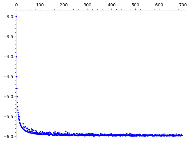
# Normalised fitness for random sequences of increasing length
def randfit(N):
    return fit(''.join([chr(97+random.randint(0,25)) for _ in range(N)]))

list_plot([randfit(k)/k for k in range(2,700)]) #fit for random sequences
# Normalised fitness for natural language text of increasing length
def randeng(text,k,N):
    return fit(text[k:k+N])

list_plot([randeng(longtxt,random.randint(0,10**5),N)/N for N in range(2,700)]) #fit for randomly chosen natural language text
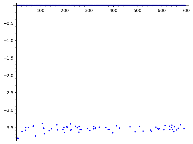
Observation
The normalised fitness (fitness divided by text length) converges to a stable value as the text length increases. For random character sequences, the value is much lower (around \(-3.5\) to \(-4.0\)) compared to natural English text (around \(-2.2\) to \(-2.5\)). This clear separation is what makes fitness-based attacks feasible: a correct decryption will have a noticeably higher fitness score than an incorrect one.
Experiment 7: Simulated Annealing Attack on Playfair#
We use simulated annealing to crack the Playfair cipher using a ciphertext-only attack. Below is the general scheme of this approach. Note that the attack is rather time consuming and it is advised for speed purposes to implement it in the compiled version of Python (or even better – write the code in C).
Generate a random key, called the ‘parent’, decipher the ciphertext using this key.
Rate the fitness of the deciphered text, store the result.
Iterate with temperature schedule:
Change the parent key slightly (e.g. swap two characters in the key at random) to get child key.
Measure the fitness of the deciphered text using the child key; set \(\Delta F\) = (fitness of child - fitness of parent).
If \(\Delta F > 0\) (fitness of child is higher than parent key), set parent = child.
If \(\Delta F < 0\) (fitness of child is worse than parent), set parent = child with probability \(e^{\Delta F / T}\).
Performance note
The simulated annealing attack is computationally intensive. For longer ciphertexts or more thorough searches, consider using %%cython magic to compile the code, or implementing in C for better performance. The cell below uses pure Python for clarity.
import copy
import random
import math

def playfairmat(key, message, encrypt=True):
    """Playfair encrypt/decrypt using a matrix directly (not a keyword string)."""
    inc = 1
    if encrypt==False:
        inc = -1
    matrix = key
    message = message.upper()
    message = message.replace(' ','')
    message = separate_same_letters(message)
    cipher_text=''
    for (l1, l2) in zip(message[0::2], message[1::2]):
        row1,col1 = indexOf(l1,matrix)
        row2,col2 = indexOf(l2,matrix)
        if row1==row2: #Rule 2, the letters are in the same row
            cipher_text += matrix[row1][(col1+inc)%5] + matrix[row2][(col2+inc)%5]
        elif col1==col2:# Rule 3, the letters are in the same column
            cipher_text += matrix[(row1+inc)%5][col1] + matrix[(row2+inc)%5][col2]
        else: #Rule 4, the letters are in a different row and column
            cipher_text += matrix[row1][col2] + matrix[row2][col1]
    return cipher_text

def swap(m1):
    m=copy.deepcopy(m1)
    x=random.randint(0,4)
    y=random.randint(0,4)
    u=random.randint(0,4)
    v=random.randint(0,4)
    a=m[x][y]
    b=m[u][v]
    m[u][v]=a
    m[x][y]=b
    return m

def modify_key(m):
    return swap(m)

def playcrack(ciph,key):
    """Simulated annealing Playfair cracker."""
    temp  = 200
    step  = 2
    count = 10000
    parent = key
    maxscore=fit(playfairmat(parent,ciph,False))
    bestscore=maxscore
    bestkey = parent

    for tt in range(temp,0,-step):
        t=tt/10.0
        for _ in range(count,0,-1):
            child=modify_key(parent)
            c=playfairmat(child,ciph,False)
            score=fit(c)
            df = score-maxscore
            if df > 0:
                parent = child
                maxscore=score
            else:
                prob = math.exp(df/t)
                r=random.random()
                if prob > r:
                    parent = child
                    maxscore=score
            if maxscore > bestscore:
                bestscore = maxscore
                bestkey = parent
                print(f'  New best score: {float(bestscore):.2f}')
    return bestscore,bestkey

print('Simulated annealing cracker defined.')
print('See the next cell for a demonstration (may take several minutes).')
Simulated annealing cracker defined.
See the next cell for a demonstration (may take several minutes).
# Prepare the ciphertext to crack
key = create_matrix('SECRET'.lower())
cc = playfairmat(key, longtxt[:400].replace('j','i'))

print(f'Ciphertext length: {len(cc)} characters')
print(f'Ciphertext (first 80): {cc[:80]}')
print()

# Start from a random key and run the cracker
parent = create_matrix('ABCDEFGHIKLMNOPQRSTUVWXYZ'.lower())
print('Running simulated annealing (this may take a while)...')
b, bk = playcrack(cc, parent)

print(f'\nFinal best score: {float(b):.2f}')
print(f'Recovered grid:')
for row in bk:
    print(' '.join(row))
print(f'\nDecrypted text (first 200 chars):')
print(playfairmat(bk, cc, False)[:200])
Ciphertext length: 404 characters
Ciphertext (first 80): ESGSRIXQMQKUGODPUZKYMKABPSGHRBEQUGISESBHSLSBFDSBELUABDWEIQLQGSISEQOVIKSKGHLEEQSF

Running simulated annealing (this may take a while)...
  New best score: -2402.82
  New best score: -2398.64
  New best score: -2397.80
  New best score: -2396.75
  New best score: -2396.67
  New best score: -2396.28
  New best score: -2395.02
  New best score: -2394.02
  New best score: -2379.24
  New best score: -2376.79
New best score: -2376.64
New best score: -2374.43
New best score: -2372.64
New best score: -2372.28
  New best score: -2363.85
  New best score: -2362.33
New best score: -2360.99
New best score: -2360.07
New best score: -2350.84
  New best score: -2349.64
  New best score: -2343.16
  New best score: -2343.13
  New best score: -2341.54
  New best score: -2337.26
  New best score: -2329.13
  New best score: -2322.96
  New best score: -2302.25
New best score: -2291.82
  New best score: -2284.44
  New best score: -2277.40
  New best score: -2205.94
  New best score: -2204.89
  New best score: -2200.59
  New best score: -2195.33
  New best score: -2191.03
  New best score: -2158.87
  New best score: -2140.24
  New best score: -2133.96
  New best score: -2133.66
  New best score: -2051.06
  New best score: -2050.36
  New best score: -2047.49
  New best score: -2033.06
  New best score: -1999.45
New best score: -1963.59
Final best score: -1963.59
Recovered grid:
S C T R E
N P U Q O
H K M L I
V X Z Y W
A D G F B

Decrypted text (first 200 chars):
REATELYPLUMPBUXCTMLXKHBFNCAMEFROTZHEREAIRHEAGAEARINGFAIBLOQRATHERONWLHCHAMIRRORANDARAZORLAYCROSXRSGFYELXLOWDCSSXSINGGOWNOQGIRDLEDWNVSUREAINEGBENTLYBEHINDHHINQTHEMHKDMORNINGAIRHEHELDTHEOIWLALOFTANDINTO
Expected result
When the simulated annealing attack converges successfully, the decrypted text should be recognisable English (from the beginning of Ulysses by James Joyce). Note that:
I and J are interchangeable (the cipher cannot distinguish them).
Filler X characters may appear where repeated letters were separated.
Multiple runs may be needed to escape local optima and find the global best key.
The attack demonstrates that the Playfair cipher, while historically important, is vulnerable to modern computational cryptanalysis using fitness-based optimisation.
Experiment 8 (Bonus): Comparing Playfair Key Space with Monoalphabetic Substitution#
We compare the theoretical key spaces of monoalphabetic substitution and the Playfair cipher, and visualise how the effective key space is affected by keyword-based construction.
from math import log10

# Key space comparison (using SageMath's built-in factorial)
mono_keyspace = factorial(26)
mono_log = float(log10(mono_keyspace))

playfair_total = factorial(25)
playfair_log = float(log10(playfair_total))

print('KEY SPACE COMPARISON')
print('=' * 50)
print(f'Monoalphabetic substitution: 26! = {float(mono_keyspace):.4e}')
print(f'  log10 = {float(mono_log):.1f} (approximately {float(mono_log):.0f} digits)')
print()
print(f'Playfair (all grids):        25! = {float(playfair_total):.4e}')
print(f'  log10 = {float(playfair_log):.1f} (approximately {float(playfair_log):.0f} digits)')
print()

# Keyword-based Playfair grids
print('Keyword-based Playfair grids (keyword length k):')
print(f'{"k":>3s}  {"Distinct grids":>20s}  {"log10":>8s}')
print('-' * 36)
for k in range(1, 16):
    n_grids = factorial(25) // factorial(25 - k)
    print(f'{int(k):>3d}  {float(n_grids):>20.4e}  {float(log10(n_grids)):>8.1f}')
KEY SPACE COMPARISON
==================================================
Monoalphabetic substitution: 26! = 4.0329e+26
  log10 = 26.6 (approximately 27 digits)

Playfair (all grids):        25! = 1.5511e+25
  log10 = 25.2 (approximately 25 digits)

Keyword-based Playfair grids (keyword length k):
  k        Distinct grids     log10
------------------------------------
  1            2.5000e+01       1.4
  2            6.0000e+02       2.8
  3            1.3800e+04       4.1
  4            3.0360e+05       5.5
  5            6.3756e+06       6.8
  6            1.2751e+08       8.1
  7            2.4227e+09       9.4
  8            4.3609e+10      10.6
  9            7.4135e+11      11.9
 10            1.1862e+13      13.1
 11            1.7793e+14      14.3
 12            2.4910e+15      15.4
 13            3.2382e+16      16.5
 14            3.8859e+17      17.6
 15            4.2745e+18      18.6
# Visualisation using SageMath bar_chart
log_sizes = [
    float(log10(26)),
    float(log10(factorial(25) // factorial(20))),
    float(log10(factorial(25) // factorial(15))),
    float(log10(factorial(25) // factorial(10))),
    playfair_log,
    mono_log
]

P = bar_chart(log_sizes, color='steelblue')
show(P, axes_labels=['Cipher type', 'log10(key space)'],
     title='Key Space Sizes: Playfair vs. Monoalphabetic Substitution',
     figsize=[10, 5])

# Print the legend
labels = ['Caesar (shift)', 'Keyword len 5', 'Keyword len 10',
          'Keyword len 15', 'Playfair (all grids)', 'Monoalphabetic (26!)']
for i, (lab, val) in enumerate(zip(labels, log_sizes)):
    print(f'  Bar {i}: {lab:>25s}  ->  log10 = {float(val):.1f}')
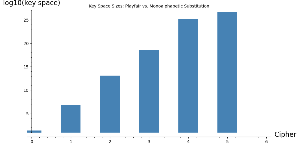
  Bar 0:            Caesar (shift)  ->  log10 = 1.4
  Bar 1:             Keyword len 5  ->  log10 = 6.8
  Bar 2:            Keyword len 10  ->  log10 = 13.1
  Bar 3:            Keyword len 15  ->  log10 = 18.6
  Bar 4:      Playfair (all grids)  ->  log10 = 25.2
  Bar 5:      Monoalphabetic (26!)  ->  log10 = 26.6
Observation
Despite having a slightly smaller total key space than monoalphabetic substitution (\(25! \approx 1.55 \times 10^{25}\) vs. \(26! \approx 4.03 \times 10^{26}\)), the Playfair cipher is significantly harder to break by simple frequency analysis because it operates on digrams rather than individual letters. However, the keyword-based construction dramatically reduces the effective key space: a keyword of length 5 yields only about \(6 \times 10^6\) distinct grids. In practice, the keyword length and dictionary constraints make the effective key space much smaller than the theoretical maximum.
Exercises#
Exercise 8.1: Grid construction
Construct the Playfair grid for the keyword QUEENSLAND. Write out the full 5\(\times\)5 grid and verify that it contains exactly 25 distinct letters (with I/J merged).
# SageMath starter code
m = create_matrix('QUEENSLAND')
for row in m:
    print(' '.join(row))
# Verify: count unique letters
all_letters = [m[i][j] for i in range(5) for j in range(5)]
print(f'Unique letters: {len(set(all_letters))}')
Hint
First remove duplicate letters from the keyword: Q, U, E, N, S, L, A, D (the second N is dropped). Then fill in the remaining 17 letters in alphabetical order: B, C, F, G, H, I, K, M, O, P, R, T, V, W, X, Y, Z.
Exercise 8.2: Encryption by hand
Using the grid from the keyword MONARCHY, encrypt the plaintext HIDE THE GOLD IN THE TREE STUMP. Show each digram, the rule applied, and the resulting ciphertext digram.
# SageMath starter code
ct, rules = encrypt_step_by_step('MONARCHY', 'HIDE THE GOLD IN THE TREE STUMP')
Hint
First prepare the digrams: HI, DE, TH, EG, OL, DI, NT, HE, TR, EX, ES, TU, MP. Note the X inserted after TRE to prevent the final E from being alone. Then apply the three rules to each pair using the MONARCHY grid.
Exercise 8.3: Proving the rectangle rule is self-inverse
Prove that the rectangle rule of the Playfair cipher is its own inverse. That is, if \(E(a, b) = (a', b')\) under the rectangle rule, then \(E(a', b') = (a, b)\).
Hint
Under the rectangle rule, \(a' = G[r_a, c_b]\) and \(b' = G[r_b, c_a]\). So \(a'\) is in row \(r_a\) and column \(c_b\), and \(b'\) is in row \(r_b\) and column \(c_a\). Since \(r_a \neq r_b\) and \(c_a \neq c_b\) (otherwise a different rule would apply), the pair \((a', b')\) also forms a rectangle. Applying the rectangle rule: \(E(a') = G[r_a, c_a] = a\) and \(E(b') = G[r_b, c_b] = b\).
Exercise 8.4: Digram frequency analysis
Encrypt a paragraph of English text (at least 200 characters) using the Playfair cipher with keyword ZEBRAS. Then:
(a) Count the 10 most frequent ciphertext digrams.
(b) Hypothesize which plaintext digrams they correspond to (using the table of common English digrams from Section 8.4.2).
(c) Verify your hypotheses by decrypting those digrams.
# SageMath starter code
ct = playfair('ZEBRAS', 'your long English text here ...')
_, di = Digrams(ct.lower())
print('Top 10 ciphertext digrams:')
for freq, dg in list(reversed(di))[:10]:
    print(f'  {dg}: {freq:.4f}')
Hint
The most frequent ciphertext digram likely corresponds to TH or HE. Build the ZEBRAS grid, find which ciphertext digram maps to TH, and check if it matches the most frequent one you observed. Remember that the Playfair cipher is a permutation on digrams, so frequency is exactly preserved.
Exercise 8.5: Fitness rating
Check for several classical ciphers (Caesar, substitution, Vigenere, Hill) how the fitness value changes from the plaintext to the ciphertext. Use for this purpose digrams, trigrams and quadgrams.
# SageMath starter code
# Build n-gram tables for n = 2, 3, 4
n2, l2, f2 = Ngrams(longtxt.replace('j','i'), 2)
n3, l3, f3 = Ngrams(longtxt.replace('j','i'), 3)
n4, l4, f4 = Ngrams(longtxt.replace('j','i'), 4)

sample_text = longtxt[:500]
# For each cipher: encrypt sample_text, compute fitness with each n-gram table
# Compare plaintext fitness vs ciphertext fitness
Hint
The Caesar and monoalphabetic substitution ciphers will show a large fitness drop for digrams and higher, because the letter-level permutation scrambles the common n-grams. The Vigenere cipher shows a moderate drop, while the Hill cipher shows the most dramatic fitness drop since it operates on blocks.
Exercise 8.6: Playfair cracker test
Based on the simulated annealing code above, write a complete program which tests the possibility of cracking the Playfair cipher for various ciphertext lengths. Focus on the aspect of length of the ciphertext required to effectively break the cipher. Read about the unicity distance and find out whether this measure is far from practical computability.
# SageMath starter code
for length in [50, 100, 200, 300, 500, 1000]:
    key = create_matrix('SECRET')
    cc = playfairmat(key, longtxt[:length].replace('j','i'))
    parent = create_matrix('ABCDEFGHIKLMNOPQRSTUVWXYZ'.lower())
    score, best_key = playcrack(cc, parent)
    decrypted = playfairmat(best_key, cc, False)
    print(f'Length {length}: score={score:.2f}, text={decrypted[:60]}...')
Hint
You should find that ciphertexts shorter than about 100 characters are very difficult to crack reliably, while 200+ characters usually suffice. The unicity distance for the Playfair cipher is relatively short due to the high redundancy of English text.
Exercise 8.7: Improving the simulated annealing attack
The simulated annealing attack in Experiment 7 uses a basic swap mutation. Improve it by implementing one or more of the following:
(a) More mutation types: Add mutations that swap two rows, swap two columns, or reverse a section of the key.
(b) Adaptive temperature schedule: Experiment with different cooling schedules (linear, geometric, etc.).
(c) Multiple restarts: Run the algorithm several times from different random starting points and keep the best result.
Test your improved attack on ciphertexts of different lengths (50, 100, 200, 500 characters) and report the success rate.
Hint
For the temperature schedule, try starting with a high temperature (e.g., \(T_0 = 20\)) and reducing it geometrically (\(T_{n+1} = \alpha T_n\) with \(\alpha \approx 0.999\)). At high temperature, the algorithm explores freely; at low temperature, it behaves like pure hill-climbing. Multiple restarts (5–10) significantly improve the chance of finding the global optimum.
Summary#
In this chapter we studied the Playfair cipher, the first practical digraphic cipher to see widespread military use.
Key concepts:
Playfair grid: A 5\(\times\)5 matrix constructed from a keyword, containing 25 letters (I and J merged). The keyword letters fill the grid first, followed by the remaining alphabet letters.
Digram preparation: Plaintext is split into letter pairs, with X inserted between repeated letters and as padding for odd-length texts.
Three encryption rules: Same row (shift right), same column (shift down), rectangle (swap columns). Decryption reverses these operations.
Digram permutation (Theorem 8.1): The Playfair cipher is a fixed permutation on the 600-element space of ordered digrams \((a, b)\) with \(a \neq b\). This means the substitution structure creates characteristic digram frequency signatures that can be exploited by cryptanalysis.
Digram frequency analysis: Because the permutation is fixed, the statistical structure of English digrams is preserved in the ciphertext. The most frequent ciphertext digrams correspond to the most frequent English digrams (TH, HE, IN, ER, AN, …).
Fitness functions: N-gram log-probability scoring provides a quantitative measure of how English-like a decrypted text is, enabling automated cryptanalysis.
Simulated annealing attack: Computational attacks use random grid perturbations guided by a fitness function, accepting worse solutions with decreasing probability to escape local optima.
Key space: The total number of Playfair grids is \(25! \approx 1.55 \times 10^{25}\), but keyword-based construction and statistical attacks reduce the effective security far below this theoretical maximum.
The Playfair cipher represents an important step in the evolution of cryptography: the transition from monographic (single-letter) to polygraphic (multi-letter) systems. In the next chapter, we will see how automated cryptanalysis techniques can be applied more broadly.
References#
Wheatstone, C. (1854). On the Reading of Cipher Despatches. Manuscript submitted to the British Foreign Office. – The original description of the cipher, unpublished during Wheatstone’s lifetime.
Friedman, W. F. (1925). Several Machine Ciphers and Methods for their Solution. Riverbank Publication No. 20. – Contains early analysis of the Playfair cipher and related systems.
Sinkov, A. (1966). Elementary Cryptanalysis: A Mathematical Approach. Mathematical Association of America. [4] – Chapter 7 provides a textbook introduction to the Playfair cipher and digram analysis.
Bauer, F. L. (2007). Decrypted Secrets: Methods and Maxims of Cryptology. 4th edition, Springer. [5] – Section 3.4 covers the Playfair cipher and its military history in detail.
Singh, S. (1999). The Code Book: The Science of Secrecy from Ancient Egypt to Quantum Cryptography. Doubleday. [3] – Chapter 2 tells the entertaining story of Wheatstone, Playfair, and Lord Palmerston.
Kahn, D. (1996). The Codebreakers: The Comprehensive History of Secret Communication from Ancient Times to the Internet. Revised edition, Scribner. – Chapter 7 provides extensive historical context on the Playfair cipher in military communications.