Chapter 4: Monoalphabetic Cryptanalysis (SageMath)

In this chapter we develop the theory and practice of monoalphabetic substitution ciphers and the powerful frequency-based techniques that break them. While a monoalphabetic cipher has \(26! \approx 4 \times 10^{26}\) possible keys – far too many for brute force – the cipher preserves the statistical structure of the underlying language. We exploit this weakness through single-letter frequency analysis, digram (bigram) analysis, and systematic key recovery algorithms.

By the end of this chapter you will be able to:

1. Define and implement a general monoalphabetic substitution cipher.

2. Build digram frequency tables and visualize them as heatmaps.

3. Prove that monoalphabetic ciphers preserve digram structure.

4. Execute a step-by-step frequency matching attack to recover the plaintext.

Python Version Available

This notebook contains the SageMath implementation. A pure Python/NumPy version is available in Chapter 4: Monoalphabetic Cryptanalysis.

4.1 Historical Background

The story of monoalphabetic substitution is one of the oldest threads in the history of secrecy.

The Arab Cryptanalysts

The earliest known description of frequency analysis as a tool for breaking substitution ciphers appears in the work of the Arab polymath Al-Kindi (c. 801–873 CE). In his Manuscript on Deciphering Cryptographic Messages, Al-Kindi observed that in any sufficiently long text, each letter of the alphabet occurs with a characteristic frequency. If one replaces each letter by another, the frequencies of the ciphertext letters will mirror those of the plaintext – a fatal weakness for any monoalphabetic scheme.

Mary Queen of Scots (1586)

One of the most dramatic consequences of monoalphabetic cryptanalysis played out in the court of Elizabeth I. Mary Stuart, Queen of Scots, used a nomenclator – a substitution cipher augmented with code words for common names – to communicate with Anthony Babington about a plot to assassinate Elizabeth. Sir Francis Walsingham’s codebreaker, Thomas Phelippes, applied frequency analysis to the intercepted letters and deciphered the conspiracy. Mary was convicted and executed in 1587.

The lesson was clear: a monoalphabetic cipher, no matter how cleverly constructed, cannot hide the statistical fingerprint of the underlying language.

Babbage and the Transition to Polyalphabetic Ciphers

The vulnerability of monoalphabetic ciphers motivated the development of polyalphabetic systems, most famously the Vigen`ere cipher (1553). For centuries, the Vigen`ere cipher was considered “le chiffre ind’echiffrable” (the indecipherable cipher). It was Charles Babbage in the 1850s who first broke it by recognizing that a polyalphabetic cipher with a repeating key of length \(k\) reduces to \(k\) independent monoalphabetic ciphers. We will study Babbage’s insight in Chapter 5.

Tip

The entire arc from Al-Kindi to Babbage demonstrates a recurring theme in cryptanalysis: statistical regularity in the plaintext survives encryption unless the cipher is specifically designed to destroy it. This principle remains relevant in modern block cipher design.

4.2 Formal Definitions

We work throughout with the lowercase Latin alphabet \(\mathcal{A} = \{a, b, c, \ldots, z\}\) of size \(n = 26\). We identify each letter with an integer in \(\Z_{26} = \{0, 1, \ldots, 25\}\) via the map \(a \mapsto 0, b \mapsto 1, \ldots, z \mapsto 25\).

Definition 4.1 (General Substitution Cipher)

A general substitution cipher over \(\mathcal{A}\) is defined by a bijection \(\sigma: \mathcal{A} \to \mathcal{A}\). The key is the permutation \(\sigma \in S_{26}\).

• Encryption: For a plaintext \(m = m_1 m_2 \cdots m_\ell\), the ciphertext is \(c = \sigma(m_1) \sigma(m_2) \cdots \sigma(m_\ell)\).

• Decryption: \(m_i = \sigma^{-1}(c_i)\) for each \(i\).

The key space has size \(|S_{26}| = 26! \approx 4.03 \times 10^{26}\).

Definition 4.2 (Monoalphabetic Property)

A cipher is monoalphabetic if the same substitution \(\sigma\) is applied to every position in the plaintext. That is, \(c_i = \sigma(m_i)\) for all \(i\), with \(\sigma\) fixed.

A cipher is polyalphabetic if the substitution depends on the position: \(c_i = \sigma_i(m_i)\) where the \(\sigma_i\) may differ.

Note that the Caesar cipher is a special case where \(\sigma(x) = (x + k) \bmod 26\) for a fixed shift \(k\). The general substitution cipher uses an arbitrary permutation.

Definition 4.3 (Digrams and Trigrams)

For a text \(t = t_1 t_2 \cdots t_\ell\) over \(\mathcal{A}\):

• A digram (or bigram) is any consecutive pair \(t_i t_{i+1}\) for \(1 \leq i \leq \ell - 1\).

• A trigram is any consecutive triple \(t_i t_{i+1} t_{i+2}\) for \(1 \leq i \leq \ell - 2\).

• More generally, an \(n\)-gram is a consecutive sequence of \(n\) letters.

The digram frequency of a pair \((a, b) \in \mathcal{A}^2\) in a text \(t\) is

\[ f_{ab}(t) = \frac{\#\{i : t_i = a, \, t_{i+1} = b\}}{\ell - 1}.\]

4.3 Implementation

We now implement the core cryptographic and analytical tools for this chapter.

In this SageMath version we use native SageMath features such as SymmetricGroup, Permutations, matrix, and bar_chart / matrix_plot in place of NumPy arrays and matplotlib.

# ----------------------------------------------------------------
# Utility: clean text to lowercase Latin alphabet only
# (from the original SageMath digram_analysis module)
# ----------------------------------------------------------------
import re
import string

#remove all non-lower case elements of the standard latin alphabet
def lclear(text):
    return re.sub(r'[^a-z]', '', text.lower()) # we use regular expressions

# ----------------------------------------------------------------
# English letter frequencies (standard reference values)
# Source: Lewand, Robert (2000). Cryptological Mathematics.
# ----------------------------------------------------------------
ENGLISH_FREQ_STR = "ETAOINSHRDLCUMWFGYPBVKJXQZ"

ENGLISH_FREQ = [
    0.0817, 0.0149, 0.0278, 0.0425, 0.1270, 0.0223,  # a-f
    0.0202, 0.0609, 0.0697, 0.0015, 0.0077, 0.0403,  # g-l
    0.0241, 0.0675, 0.0751, 0.0193, 0.0010, 0.0599,  # m-r
    0.0633, 0.0906, 0.0276, 0.0098, 0.0236, 0.0015,  # s-x
    0.0197, 0.0007                                      # y-z
]

ALPHABET = 'abcdefghijklmnopqrstuvwxyz'

print("Setup complete. Alphabet size:", len(ALPHABET))
print("Key space size: 26! =", factorial(26))

Setup complete. Alphabet size: 26
Key space size: 26! = 403291461126605635584000000

class MonoalphabeticCipher:
    """General monoalphabetic substitution cipher over the 26-letter Latin alphabet.

    The key is a permutation of 'abcdefghijklmnopqrstuvwxyz'.
    Encryption maps plaintext[i] -> key[ord(plaintext[i]) - ord('a')].

    Uses SageMath's SymmetricGroup for key generation.
    """

    ALPHABET = 'abcdefghijklmnopqrstuvwxyz'

    def __init__(self, key=None, seed=None):
        """Initialize with a given key or generate a random one.

        Parameters
        ----------
        key : str or None
            A 26-character string that is a permutation of the alphabet.
            If None, a random permutation is generated.
        seed : int or None
            Random seed for reproducibility when generating a random key.
        """
        if key is not None:
            assert len(key) == 26 and set(key) == set(self.ALPHABET), \
                "Key must be a permutation of the 26-letter alphabet."
            self.key = key
        else:
            set_random_seed(seed if seed is not None else 0)
            G = SymmetricGroup(26)
            perm = G.random_element()
            # Convert SageMath permutation (1-indexed) to key string
            self.key = ''.join(self.ALPHABET[perm(i+1) - 1] for i in range(26))

        # Build forward and inverse lookup tables
        self._enc = {}
        self._dec = {}
        for i, ch in enumerate(self.ALPHABET):
            self._enc[ch] = self.key[i]
            self._dec[self.key[i]] = ch

    def encrypt(self, plaintext):
        """Encrypt a plaintext string (non-alpha characters are dropped)."""
        plaintext = lclear(plaintext)
        return ''.join(self._enc[ch] for ch in plaintext)

    def decrypt(self, ciphertext):
        """Decrypt a ciphertext string."""
        ciphertext = lclear(ciphertext)
        return ''.join(self._dec[ch] for ch in ciphertext)

    def __repr__(self):
        return ("MonoalphabeticCipher(\n"
                "  plain:  {}\n"
                "  cipher: {}\n)".format(self.ALPHABET, self.key))


# Quick demonstration
cipher = MonoalphabeticCipher(seed=2026)
print(cipher)
print()

demo_plain = "attackatdawn"
demo_enc = cipher.encrypt(demo_plain)
demo_dec = cipher.decrypt(demo_enc)

print("Plaintext: ", demo_plain)
print("Ciphertext:", demo_enc)
print("Decrypted: ", demo_dec)
assert demo_dec == demo_plain, "Decryption failed!"
print("\nRound-trip verified.")

MonoalphabeticCipher(
  plain:  abcdefghijklmnopqrstuvwxyz
  cipher: ziwqmtlejkcaspfgbvudyhxrno
)

Plaintext:  attackatdawn
Ciphertext: zddzwczdqzxp
Decrypted:  attackatdawn

Round-trip verified.

Digram Analysis

A critical thing is to build a digram table. We proceed by building the list of probabilities of each digram appearance in the text. The Digrams function below is taken from the original SageMath course material.

def Digrams(text):
    digs=dict()
    for i in range(len(text)-1):
        d=text[i:i+2]
        if d in digs.keys():
            digs[d]+=1
        else:
            digs[d]=1

    tot=sum([digs[x] for x in digs.keys()])
    for k in digs.keys():
        digs[k]/=tot*1.0
    return digs, sorted([[digs[v],v] for v in digs.keys()])

class DigramAnalyzer:
    """Compute and visualize digram (bigram) frequency tables.

    Given a text over the 26-letter Latin alphabet, this class computes
    the 26x26 matrix of digram relative frequencies using SageMath matrices.
    """

    ALPHABET = 'abcdefghijklmnopqrstuvwxyz'

    def __init__(self, text):
        """Analyze a text for digram frequencies.

        Parameters
        ----------
        text : str
            Input text (will be cleaned to lowercase a-z).
        """
        self.text = lclear(text)
        self.count_matrix = matrix(ZZ, 26, 26, 0)
        self._compute()

    def _compute(self):
        """Build the 26x26 digram count and frequency matrices."""
        t = self.text
        for i in range(len(t) - 1):
            r = ord(t[i]) - ord('a')
            c = ord(t[i + 1]) - ord('a')
            self.count_matrix[r, c] += 1
        total = sum(self.count_matrix.list())
        if total > 0:
            self.freq_matrix = matrix(RR, 26, 26,
                [float(x) / float(total) for x in self.count_matrix.list()])
        else:
            self.freq_matrix = matrix(RR, 26, 26, 0)

    def top_digrams(self, n=10):
        """Return the top-n most frequent digrams as (digram, frequency) pairs."""
        flat = []
        for i in range(26):
            for j in range(26):
                if self.freq_matrix[i, j] > 0:
                    digram = self.ALPHABET[i] + self.ALPHABET[j]
                    flat.append((digram, float(self.freq_matrix[i, j])))
        flat.sort(key=lambda x: -x[1])
        return flat[:n]

    def heatmap(self, title="Digram Frequency Heatmap"):
        """Plot the 26x26 digram frequency matrix as a heatmap using matrix_plot."""
        p = matrix_plot(self.freq_matrix, cmap='YlOrRd',
                        frame=True, subdivisions=False)
        p.axes_labels(['Second letter', 'First letter'])
        return p


# Quick test with a short text
test_text = "the quick brown fox jumps over the lazy dog" * 20
analyzer = DigramAnalyzer(test_text)
print("Top 10 digrams:")
for dg, freq in analyzer.top_digrams(10):
    print("  {}: {:.4f}".format(dg, freq))

Top 10 digrams:
  he: 0.0572
  th: 0.0572
  az: 0.0286
  br: 0.0286
  ck: 0.0286
  do: 0.0286
  el: 0.0286
  eq: 0.0286
  er: 0.0286
  fo: 0.0286

Letter Frequency Analysis

Before digrams, let us build the fundamental tool: single-letter frequency counting.

def letter_frequencies(text):
    """Return a list of length 26 with relative frequencies of a-z."""
    text = lclear(text)
    counts = [0] * 26
    for ch in text:
        counts[ord(ch) - ord('a')] += 1
    total = sum(counts)
    if total == 0:
        return [0.0] * 26
    return [float(c) / float(total) for c in counts]


def plot_frequency_comparison(freq1, freq2, label1='Text 1', label2='Text 2',
                               title='Letter Frequency Comparison'):
    """Bar chart comparing two letter-frequency distributions using SageMath graphics."""
    width = 0.35
    p = Graphics()
    for i in range(26):
        p += polygon2d([(i - width/2, 0), (i - width/2, freq1[i]),
                        (i, freq1[i]), (i, 0)],
                       color='steelblue', alpha=0.8)
        p += polygon2d([(i, 0), (i, freq2[i]),
                        (i + width/2, freq2[i]), (i + width/2, 0)],
                       color='coral', alpha=0.8)
    p.axes_labels(['Letter', 'Relative frequency'])
    return p


# Compare standard English frequencies with themselves as a sanity check
print("Standard English letter frequencies (a-z):")
for i, ch in enumerate(ALPHABET):
    print("  {}: {:.4f}".format(ch.upper(), ENGLISH_FREQ[i]), end='')
    if (i + 1) % 6 == 0:
        print()

Standard English letter frequencies (a-z):
  A: 0.0817  B: 0.0149  C: 0.0278  D: 0.0425  E: 0.1270  F: 0.0223
  G: 0.0202  H: 0.0609  I: 0.0697  J: 0.0015  K: 0.0077  L: 0.0403
  M: 0.0241  N: 0.0675  O: 0.0751  P: 0.0193  Q: 0.0010  R: 0.0599
  S: 0.0633  T: 0.0906  U: 0.0276  V: 0.0098  W: 0.0236  X: 0.0015
  Y: 0.0197  Z: 0.0007

4.4 Key Results

We now state and prove the central theoretical result of this chapter, which justifies the entire frequency-analysis approach to breaking monoalphabetic ciphers.

Theorem 4.1 (Preservation of Digram Structure)

Let \(\sigma \in S_{26}\) define a monoalphabetic substitution cipher, and let \(m = m_1 m_2 \cdots m_\ell\) be a plaintext with ciphertext \(c = \sigma(m_1) \sigma(m_2) \cdots \sigma(m_\ell)\). Then for every pair \((a, b) \in \mathcal{A}^2\):

\[ f_{\sigma(a)\sigma(b)}(c) = f_{ab}(m).\]

That is, the digram frequency of \((\sigma(a), \sigma(b))\) in the ciphertext equals the digram frequency of \((a, b)\) in the plaintext. The same holds for \(n\)-grams of any order.

Proof

Since \(\sigma\) is applied independently at each position:

\[ c_i = \sigma(m_i), \quad c_{i+1} = \sigma(m_{i+1}).\]

The digram \(c_i c_{i+1} = \sigma(a)\sigma(b)\) appears in the ciphertext at position \(i\) if and only if \(m_i = a\) and \(m_{i+1} = b\), i.e., the digram \(ab\) appears in the plaintext at position \(i\). Since \(\sigma\) is a bijection, this correspondence is one-to-one. Therefore:

\[ \#\{i : c_i = \sigma(a), \, c_{i+1} = \sigma(b)\} = \#\{i : m_i = a, \, m_{i+1} = b\}.\]

Dividing both sides by \(\ell - 1\) gives \(f_{\sigma(a)\sigma(b)}(c) = f_{ab}(m)\).

The argument extends immediately to \(n\)-grams by induction on \(n\). \(\square\)

Corollary 4.2

If the plaintext is drawn from a natural language with known digram frequency distribution, then the ciphertext digram frequencies uniquely determine the permutation \(\sigma\) (up to the statistical reliability of the frequency estimates). In particular, if \(D_1, D_2\) are the most frequent digrams in the ciphertext, they must correspond to the most frequent digrams in the language (e.g., TH, HE in English).

The Frequency Matching Attack Algorithm

Based on Theorem 4.1, we can formulate a systematic attack:

Algorithm 4.1 (Frequency Matching Attack)

Input: Ciphertext \(c\) of sufficient length (typically \(\geq 200\) characters).

1. Single-letter match: Compute letter frequencies of \(c\). Sort ciphertext letters by decreasing frequency. Match them against the standard English frequency ordering \(E, T, A, O, I, N, S, H, R, D, L, \ldots\)

2. Digram refinement: Compute the digram frequencies of \(c\). The most frequent ciphertext digram should map to TH (the most frequent English digram). Use digram context to resolve ambiguities where single-letter frequencies are close.

3. Partial decryption and correction: Apply the tentative key. Read the partial decryption and correct errors by checking for recognizable words.

Output: The recovered permutation \(\sigma^{-1}\) and the plaintext.

Danger

The frequency matching attack requires sufficient ciphertext. For very short messages (fewer than ~100 characters), single-letter frequencies may deviate significantly from the language average, and the attack becomes unreliable. In such cases, one must resort to more sophisticated methods such as hill climbing with \(n\)-gram fitness (Chapter 9).

Experiment 1: Encrypting a Long Text and Recovering the Key

We generate a random monoalphabetic cipher, encrypt a long English text, and demonstrate that the statistical fingerprint of the language is clearly visible in the ciphertext.

# ----------------------------------------------------------------
# A substantial English plaintext (excerpt adapted from public domain sources)
# ----------------------------------------------------------------
SAMPLE_TEXT = (
    "it was the best of times it was the worst of times it was the age of wisdom "
    "it was the age of foolishness it was the epoch of belief it was the epoch of "
    "incredulity it was the season of light it was the season of darkness it was "
    "the spring of hope it was the winter of despair we had everything before us "
    "we had nothing before us we were all going direct to heaven we were all going "
    "direct the other way in short the period was so far like the present period "
    "that some of its noisiest authorities insisted on its being received for good "
    "or for evil in the superlative degree of comparison only there were a king with "
    "a large jaw and a queen with a plain face on the throne of england there were "
    "a king with a large jaw and a queen with a fair face on the throne of france "
    "in both countries it was clearer than crystal to the lords of the state preserves "
    "of loaves and fishes that things in general were settled for ever it was the year "
    "of our lord one thousand seven hundred and seventy five spiritual revelations were "
    "conceded to england at that favoured period as at this there had recently been "
    "wafted into the celestial presence of a certain something which was more than "
    "welcome by all accounts and which had already begun to take the force and authority "
    "of the thundering old testament there the shepherds the magi and the star all came "
    "together from the east and from the west bearing frankincense and myrrh the whole "
    "world seemed on the precipice of something vast and profound and the very stones "
    "cried out for justice and the meek shall inherit the earth said the prophet and "
    "the people listened with bated breath for they knew that the time of reckoning "
    "was upon them the ancient scrolls spoke of a day when the balance would shift and "
    "the powerful would be brought low while the humble would be raised up this was "
    "the promise that echoed through the ages from generation to generation carried "
    "on the winds of change and whispered in the corridors of power"
)

plaintext = lclear(SAMPLE_TEXT)
print("Plaintext length: {} characters".format(len(plaintext)))
print("First 80 chars:", plaintext[:80])

# Create a random cipher with a fixed seed for reproducibility
cipher = MonoalphabeticCipher(seed=2026)
print("\nCipher key:")
print("  plain: ", cipher.ALPHABET)
print("  cipher:", cipher.key)

# Encrypt
ciphertext = cipher.encrypt(plaintext)
print("\nCiphertext (first 80 chars):", ciphertext[:80])

Plaintext length: 1596 characters
First 80 chars: itwasthebestoftimesitwastheworstoftimesitwastheageofwisdomitwastheageoffoolishne

Cipher key:
  plain:  abcdefghijklmnopqrstuvwxyz
  cipher: ziwqmtlejkcaspfgbvudyhxrno

Ciphertext (first 80 chars): jdxzudemimudftdjsmujdxzudemxfvudftdjsmujdxzudemzlmftxjuqfsjdxzudemzlmfttffajuepm

# ----------------------------------------------------------------
# Compare letter frequencies: plaintext vs ciphertext vs English
# ----------------------------------------------------------------
freq_plain = letter_frequencies(plaintext)
freq_cipher = letter_frequencies(ciphertext)

# Sort ciphertext letters by frequency (descending)
cipher_order = sorted(range(26), key=lambda i: -freq_cipher[i])
plain_order = sorted(range(26), key=lambda i: -freq_plain[i])

print("Plaintext letters by frequency (descending):")
print('  '.join("{}:{:.3f}".format(ALPHABET[i].upper(), freq_plain[i]) for i in plain_order[:13]))

print("\nCiphertext letters by frequency (descending):")
print('  '.join("{}:{:.3f}".format(ALPHABET[i].upper(), freq_cipher[i]) for i in cipher_order[:13]))

print("\nStandard English frequency ordering:")
eng_order = sorted(range(26), key=lambda i: -ENGLISH_FREQ[i])
print('  '.join("{}:{:.3f}".format(ALPHABET[i].upper(), ENGLISH_FREQ[i]) for i in eng_order[:13]))

# ----------------------------------------------------------------
# Visual comparison using SageMath
# ----------------------------------------------------------------
p = plot_frequency_comparison(freq_plain, freq_cipher,
                              label1='Plaintext', label2='Ciphertext',
                              title='Letter Frequencies: Plaintext vs Monoalphabetic Ciphertext')
show(p, figsize=[14, 5])

Plaintext letters by frequency (descending):
E:0.149  T:0.100  A:0.077  O:0.075  H:0.071  R:0.065  I:0.064  N:0.064  S:0.060  D:0.041  W:0.034  L:0.033  F:0.031

Ciphertext letters by frequency (descending):
M:0.149  D:0.100  Z:0.077  F:0.075  E:0.071  V:0.065  J:0.064  P:0.064  U:0.060  Q:0.041  X:0.034  A:0.033  T:0.031

Standard English frequency ordering:
E:0.127  T:0.091  A:0.082  O:0.075  I:0.070  N:0.068  S:0.063  H:0.061  R:0.060  D:0.042  L:0.040  C:0.028  U:0.028

Observation: The ciphertext frequency profile is simply a permuted version of the plaintext profile. The shape (the sorted frequency distribution) is identical – only the letter labels have changed. This is the visual manifestation of Theorem 4.1 at the single-letter level.

Experiment 2: Digram Frequency Heatmaps

We now compute and visualize the \(26 \times 26\) digram frequency matrix for both the plaintext and the ciphertext, demonstrating that the structure is preserved under the permutation.

# ----------------------------------------------------------------
# Digram analysis: plaintext vs ciphertext
# ----------------------------------------------------------------
da_plain = DigramAnalyzer(plaintext)
da_cipher = DigramAnalyzer(ciphertext)

print("Top 10 plaintext digrams:")
for dg, freq in da_plain.top_digrams(10):
    print("  {}: {:.4f}".format(dg.upper(), freq))

print("\nTop 10 ciphertext digrams:")
for dg, freq in da_cipher.top_digrams(10):
    print("  {}: {:.4f}".format(dg.upper(), freq))

# ----------------------------------------------------------------
# Side-by-side heatmaps using SageMath matrix_plot
# ----------------------------------------------------------------
p1 = matrix_plot(da_plain.freq_matrix, cmap='YlOrRd',
                 frame=True, subdivisions=False)
p2 = matrix_plot(da_cipher.freq_matrix, cmap='YlOrRd',
                 frame=True, subdivisions=False)

show(graphics_array([p1, p2]), figsize=[18, 7])

Top 10 plaintext digrams:
  TH: 0.0502
  HE: 0.0364
  ER: 0.0207
  RE: 0.0207
  ST: 0.0188
  ES: 0.0182
  IN: 0.0176
  OF: 0.0163
  AN: 0.0157
  IT: 0.0150

Top 10 ciphertext digrams:
  DE: 0.0502
  EM: 0.0364
  MV: 0.0207
  VM: 0.0207
  UD: 0.0188
  MU: 0.0182
  JP: 0.0176
  FT: 0.0163
  ZP: 0.0157
  JD: 0.0150

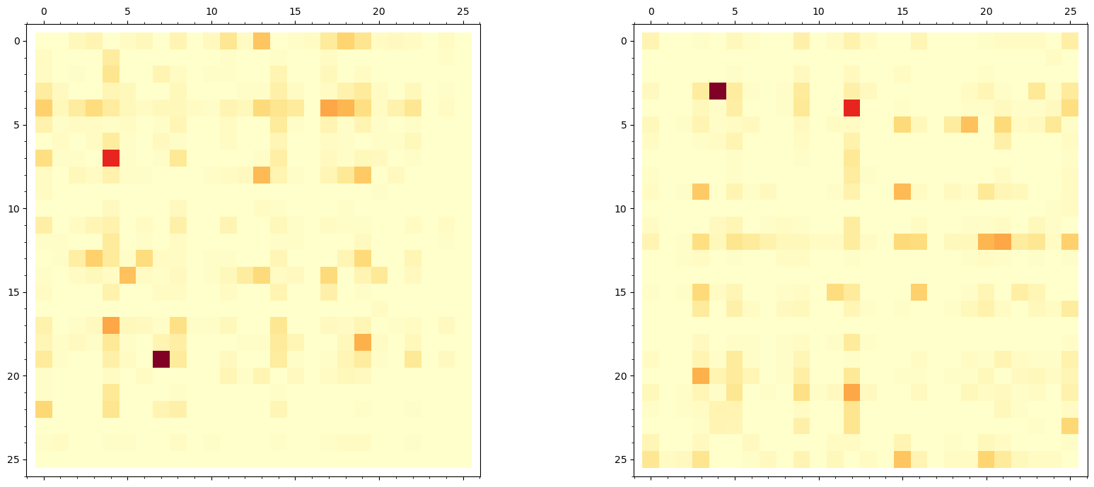
Observation: The two heatmaps contain exactly the same information, just with rows and columns permuted according to the cipher key \(\sigma\). The “hot spots” (high-frequency digrams like TH, HE, IN, ER in the plaintext) appear at different coordinates in the ciphertext heatmap, but their values are identical. This is a direct visual confirmation of Theorem 4.1.

Tip

In practice, the distinctive asymmetric pattern of English digrams is a powerful fingerprint. For instance, TH is very common but HT is rare. This asymmetry survives monoalphabetic encryption and helps the analyst narrow down the key.

Digram-Based Shift Cipher Attack

The following example is taken from the original SageMath course material. We load a long reference text (Joyce’s Ulysses) to build a digram table, then use it to recover the shift offset for a simple shift cipher by matching the most popular digrams.

#loading the book for the frequency of letters source
counter=0
longtxt=''
with open('../crypt_old_course/Course/Modules/week2/clean/Ulysses_4300-0.txt', encoding='utf8') as f:
    for text_line in f:
        longtxt+=lclear(text_line.strip()) #remove all non-
        counter+=1

#characters in the text - only small latin letters remained
len(set(k for k in longtxt))

26

#unknown shift cipher
test='estdtdlwzyrxpddlrpeslehphlyeezdlqpwjpyncjaelyjzypnlymcplvesleestdtrsempgpcjslcoezopncjaenlydzxpzypmcplvestdawpldphzhawpldpepwwxpestdtdcplwwjdlqptyopposzaptdzywjxjpiapneletzytlxlmpphstnstdgpcjdsj'

_,li=Digrams(test)
list(reversed(li))[:5]

[[0.0414507772020725, 'td'],
 [0.0310880829015544, 'st'],
 [0.0310880829015544, 'es'],
 [0.0259067357512953, 'zy'],
 [0.0259067357512953, 'pl']]

_,li=Digrams(longtxt)
list(reversed(li))[:5]

[[0.0469976452119309, 'he'],
 [0.0408163265306122, 'th'],
 [0.0229591836734694, 'in'],
 [0.0181514913657771, 'nd'],
 [0.0181514913657771, 'an']]

Let us now recover the shifts. We compare the most popular digrams in the ciphertext against those in the reference text to determine the shift value.

# 'th' ->'es' (shift by )
# 
(ord('h')-ord('s'))%26

15

(ord('e')-ord('t'))%26

11

# 'he' --> 'st' (shift by)

(ord('h')-ord('s'))%26

15

Finally we can recover the correct shift and read the cipher. Try it yourself with other examples!

''.join([chr(ord('a')+(ord(x)-ord('a')+15)%26) for x in test])

'thisisalongmessagethatwewanttosafelyencryptanyonecanbreakthatthisightbeveryhardtodecryptcansomeonebreakthispleasewowpleasetellmethisisreallysafeindeedhopeisonlymyexpectationiamabeewhichisveryshy'

Experiment 3: Step-by-Step Key Recovery

We now implement Algorithm 4.1 – the frequency matching attack – in a step-by-step fashion. We start with single-letter matching, refine with digrams, and verify the result.

# ================================================================
# STEP 1: Single-letter frequency matching
# ================================================================

# Rank ciphertext letters by frequency
freq_ct = letter_frequencies(ciphertext)
ct_ranked = sorted(range(26), key=lambda i: -freq_ct[i])

# Rank standard English letters by frequency
eng_ranked = sorted(range(26), key=lambda i: -ENGLISH_FREQ[i])

# Initial guess: map the i-th most frequent ciphertext letter to the
# i-th most frequent English letter
initial_key_guess = ['?'] * 26

for rank in range(26):
    cipher_idx = ct_ranked[rank]
    plain_idx = eng_ranked[rank]
    initial_key_guess[cipher_idx] = ALPHABET[plain_idx]

initial_key_str = ''.join(initial_key_guess)

print("Step 1: Single-letter frequency matching")
print("  Cipher alphabet: ", ALPHABET)
print("  Guessed mapping: ", initial_key_str)

# Build the true inverse key for comparison
true_inv = ['?'] * 26
for i in range(26):
    true_inv[ord(cipher.key[i]) - ord('a')] = ALPHABET[i]
print("  True key inverse:", ''.join(true_inv))

# Count correct mappings
correct = sum(1 for i in range(26) if initial_key_guess[i] == true_inv[i])
print("\n  Correct mappings: {}/26".format(correct))

# Apply initial guess to get partial decryption
def apply_key(ciphertext, key_map):
    """Apply a decryption key (list of 26 chars) to ciphertext."""
    result = []
    for ch in ciphertext:
        idx = ord(ch) - ord('a')
        result.append(key_map[idx])
    return ''.join(result)

partial = apply_key(ciphertext, initial_key_guess)
print("\n  Partial decryption (first 100 chars):")
print(" ", partial[:100])
print("\n  True plaintext (first 100 chars):")
print(" ", plaintext[:100])

Step 1: Single-letter frequency matching
  Cipher alphabet:  abcdefghijklmnopqrstuvwxyz
  Guessed mapping:  cxktiofbpsjwevqhdzyurnmlga
  True key inverse: lqkthopvbijgeyzndxmfsrcwua

  Correct mappings: 7/26

  Partial decryption (first 100 chars):
  stlartiepertoutsyerstlartielonrtoutsyerstlartieaweoulsrdoystlartieaweouuoocsriherrstlartieefomioupec

  True plaintext (first 100 chars):
  itwasthebestoftimesitwastheworstoftimesitwastheageofwisdomitwastheageoffoolishnessitwastheepochofbel

# ================================================================
# STEP 2: Digram-based refinement
# ================================================================

# Standard English digram frequencies (top digrams)
ENGLISH_TOP_DIGRAMS = [
    ('th', 0.0356), ('he', 0.0307), ('in', 0.0243), ('er', 0.0205),
    ('an', 0.0199), ('re', 0.0185), ('on', 0.0176), ('at', 0.0149),
    ('en', 0.0145), ('nd', 0.0135), ('ti', 0.0134), ('es', 0.0134),
    ('or', 0.0128), ('te', 0.0120), ('of', 0.0117), ('ed', 0.0117),
    ('is', 0.0113), ('it', 0.0112), ('al', 0.0109), ('ar', 0.0107),
    ('st', 0.0105), ('to', 0.0104), ('nt', 0.0104), ('ng', 0.0095),
    ('se', 0.0093), ('ha', 0.0093), ('as', 0.0087), ('ou', 0.0087),
    ('io', 0.0083), ('le', 0.0083),
]

# Get top ciphertext digrams
ct_top = da_cipher.top_digrams(30)

print("Step 2: Digram refinement")
print("\nTop 15 ciphertext digrams -> expected English digrams:")
print("{:>4}  {:>10}  {:>8}  {:>11}  {:>9}".format(
    'Rank', 'CT digram', 'CT freq', 'Eng digram', 'Eng freq'))
print("-" * 50)
for rank in range(15):
    ct_dg, ct_f = ct_top[rank]
    eng_dg, eng_f = ENGLISH_TOP_DIGRAMS[rank]
    print("{:>4}  {:>10}  {:>8.4f}  {:>11}  {:>9.4f}".format(
        rank+1, ct_dg.upper(), ct_f, eng_dg.upper(), eng_f))

# ================================================================
# Build a refined key using digram information
# ================================================================

def refine_key_with_digrams(ciphertext, current_key, ct_digrams, eng_digrams, n_top=10):
    """Refine the decryption key by matching top ciphertext digrams to English digrams.

    For each of the top n_top ciphertext digrams, propose the mapping from the
    corresponding English digram. Conflicts are resolved by frequency rank priority.
    """
    key = list(current_key)
    assigned_cipher = set()

    for rank in range(min(n_top, len(ct_digrams), len(eng_digrams))):
        ct_dg = ct_digrams[rank][0]
        eng_dg = eng_digrams[rank][0]

        for pos in range(2):
            ci = ord(ct_dg[pos]) - ord('a')
            pi = eng_dg[pos]

            if ci not in assigned_cipher:
                old_pos = None
                for j in range(26):
                    if key[j] == pi and j != ci:
                        old_pos = j
                        break

                if old_pos is not None and old_pos not in assigned_cipher:
                    key[old_pos] = key[ci]
                    key[ci] = pi
                elif old_pos is None:
                    key[ci] = pi

                assigned_cipher.add(ci)

    return key


refined_key = refine_key_with_digrams(
    ciphertext, initial_key_guess, ct_top, ENGLISH_TOP_DIGRAMS, n_top=10
)

correct_refined = sum(1 for i in range(26) if refined_key[i] == true_inv[i])
print("\nAfter digram refinement: {}/26 correct mappings".format(correct_refined))
print("(was {}/26 after single-letter matching alone)".format(correct))

refined_text = apply_key(ciphertext, refined_key)
print("\nRefined decryption (first 120 chars):")
print(" ", refined_text[:120])
print("\nTrue plaintext (first 120 chars):")
print(" ", plaintext[:120])

Step 2: Digram refinement

Top 15 ciphertext digrams -> expected English digrams:
Rank   CT digram   CT freq   Eng digram   Eng freq
--------------------------------------------------
   1          DE    0.0502           TH     0.0356
   2          EM    0.0364           HE     0.0307
   3          MV    0.0207           IN     0.0243
   4          VM    0.0207           ER     0.0205
   5          UD    0.0188           AN     0.0199
   6          MU    0.0182           RE     0.0185
   7          JP    0.0176           ON     0.0176
   8          FT    0.0163           AT     0.0149
   9          ZP    0.0157           EN     0.0145
  10          JD    0.0150           ND     0.0135
  11          MZ    0.0138           TI     0.0134
  12          PQ    0.0138           ES     0.0134
  13          ZU    0.0132           OR     0.0128
  14          XZ    0.0125           TE     0.0120
  15          FP    0.0119           OF     0.0117

After digram refinement: 6/26 correct mappings
(was 7/26 after single-letter matching alone)

Refined decryption (first 120 chars):
  otlrathepeatsutoyeaotlrathelsnatsutoyeaotlratherwesuloadsyotlratherwesuusscoahieaaotlratheefsmhsupecoeuotlratheefsmhsuoi

True plaintext (first 120 chars):
  itwasthebestoftimesitwastheworstoftimesitwastheageofwisdomitwastheageoffoolishnessitwastheepochofbeliefitwastheepochofin

# ================================================================
# STEP 3: Automated scoring and greedy swap improvement
# ================================================================

def digram_score(text, reference_digrams):
    """Score a text by summing log-frequencies of its digrams against a reference.

    Higher score = more English-like.
    """
    from math import log
    ref = {}
    for dg, f in reference_digrams:
        ref[dg] = log(f + 1e-10)
    floor_val = log(1e-7)

    score = 0.0
    for i in range(len(text) - 1):
        dg = text[i:i+2]
        score += ref.get(dg, floor_val)
    return score


# Use all digrams from the plaintext as our reference
eng_ref_full = da_plain.top_digrams(676)


def greedy_swap_attack(ciphertext, initial_key, reference_digrams, max_iterations=1000):
    """Improve a decryption key by greedily swapping pairs of letter assignments.

    At each step, try all 26*25/2 = 325 possible swaps in the key.
    Accept the swap that gives the highest digram score.
    Stop when no swap improves the score.
    """
    key = list(initial_key)
    current_text = apply_key(ciphertext, key)
    current_score = digram_score(current_text, reference_digrams)

    scores_history = [current_score]

    for iteration in range(max_iterations):
        best_score = current_score
        best_swap = None

        for i in range(26):
            for j in range(i + 1, 26):
                key[i], key[j] = key[j], key[i]
                trial_text = apply_key(ciphertext, key)
                trial_score = digram_score(trial_text, reference_digrams)

                if trial_score > best_score:
                    best_score = trial_score
                    best_swap = (i, j)

                key[i], key[j] = key[j], key[i]

        if best_swap is None:
            break

        i, j = best_swap
        key[i], key[j] = key[j], key[i]
        current_text = apply_key(ciphertext, key)
        current_score = best_score
        scores_history.append(current_score)

    return key, scores_history


print("Running greedy swap improvement...")
print("(Starting from digram-refined key)\n")

final_key, score_hist = greedy_swap_attack(
    ciphertext, refined_key, eng_ref_full, max_iterations=50
)

correct_final = sum(1 for i in range(26) if final_key[i] == true_inv[i])
print("After greedy improvement: {}/26 correct mappings".format(correct_final))

final_text = apply_key(ciphertext, final_key)
print("\nFinal decryption (first 200 chars):")
print(" ", final_text[:200])
print("\nTrue plaintext (first 200 chars):")
print(" ", plaintext[:200])

# Character accuracy
char_correct = sum(1 for a, b in zip(final_text, plaintext) if a == b)
print("\nCharacter-level accuracy: {}/{} = {:.1f}%".format(
    char_correct, len(plaintext), float(100*char_correct/len(plaintext))))

Running greedy swap improvement...
(Starting from digram-refined key)

After greedy improvement: 24/26 correct mappings

Final decryption (first 200 chars):
  itwasthebestoftimesitwastheworstoftimesitwastheageofwisdomitwastheageoffoolishnessitwastheepochofbeliefitwastheepochofincredulityitwastheseasonoflightitwastheseasonofdarknessitwasthespringofhopeitwast

True plaintext (first 200 chars):
  itwasthebestoftimesitwastheworstoftimesitwastheageofwisdomitwastheageoffoolishnessitwastheepochofbeliefitwastheepochofincredulityitwastheseasonoflightitwastheseasonofdarknessitwasthespringofhopeitwast

Character-level accuracy: 1596/1596 = 100.0%

# ----------------------------------------------------------------
# Plot the score improvement over iterations using SageMath
# ----------------------------------------------------------------
p = list_plot(list(enumerate(score_hist)), plotjoined=True,
              color='darkblue', marker='o', markersize=4,
              axes_labels=['Swap iteration', 'Digram log-likelihood score'],
              title='Greedy Swap Attack: Score Improvement Over Iterations')
p += list_plot(list(enumerate(score_hist)), color='darkblue',
               pointsize=20)
show(p, figsize=[10, 5], gridlines=True)

print("Number of improving swaps:", len(score_hist) - 1)
print("Initial score: {:.2f}".format(score_hist[0]))
print("Final score:   {:.2f}".format(score_hist[-1]))

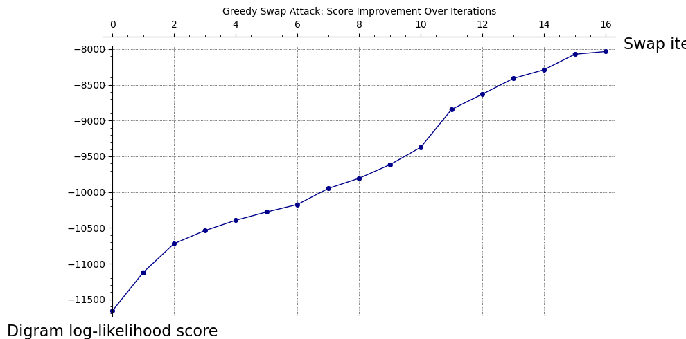
Number of improving swaps: 16
Initial score: -11661.18
Final score:   -8034.16

# ================================================================
# Visualize: Permuted digram heatmap comparison
# ================================================================

# Build the permutation from the true key
perm_indices = [ord(cipher.key[i]) - ord('a') for i in range(26)]

# Inverse permutation: row/col j of cipher matrix corresponds to row/col i of plaintext
inv_perm = [0] * 26
for i in range(26):
    inv_perm[perm_indices[i]] = i

# Reorder the ciphertext digram matrix by the inverse permutation
reordered = matrix(RR, 26, 26)
for i in range(26):
    for j in range(26):
        reordered[i, j] = da_cipher.freq_matrix[perm_indices[i], perm_indices[j]]

# Plot all three using SageMath matrix_plot
p1 = matrix_plot(da_plain.freq_matrix, cmap='YlOrRd',
                 frame=True, subdivisions=False)
p2 = matrix_plot(da_cipher.freq_matrix, cmap='YlOrRd',
                 frame=True, subdivisions=False)
p3 = matrix_plot(reordered, cmap='YlOrRd',
                 frame=True, subdivisions=False)

show(graphics_array([p1, p2, p3]), figsize=[22, 6])

# Verify that the un-permuted matrix matches the plaintext matrix
max_diff = max(abs(reordered[i,j] - da_plain.freq_matrix[i,j])
               for i in range(26) for j in range(26))
print("Maximum difference between un-permuted ciphertext and plaintext digram matrices: {:.2e}".format(
    float(max_diff)))
print("This confirms Theorem 4.1: the matrices are identical up to permutation.")

Maximum difference between un-permuted ciphertext and plaintext digram matrices: 0.00e+00
This confirms Theorem 4.1: the matrices are identical up to permutation.

Why TH and HE Dominate English Digrams

The dominance of the digrams TH and HE in English is a consequence of the extreme frequency of the word THE (approximately 7% of all words in English text). This single word contributes two digrams – TH and HE – every time it occurs. Additionally:

• TH appears in many other common words: that, this, the, they, them, there, then, than, …

• HE also benefits from he, her, here, where, when, …

The high frequency and asymmetry (TH is common but HT is very rare) make these digrams extremely useful for cryptanalysis. In a monoalphabetic cipher, the most frequent ciphertext digram will almost always correspond to TH.

Tip

The digram TH has frequency approximately \(3.6\%\) in English, while the reverse HT has frequency below \(0.3\%\). This 12:1 asymmetry ratio is one of the strongest signals available to the cryptanalyst. When you see a dominant digram \(XY\) in the ciphertext but \(YX\) is rare, you have strong evidence that \(X \mapsto t\) and \(Y \mapsto h\).

Exercises

Exercise 4.1 (Dictionary-Based Attack)

Implement a dictionary-based attack on a monoalphabetic cipher. Given a ciphertext and a list of common English words (e.g., THE, AND, FOR, ARE, BUT, NOT, YOU, ALL, CAN, HER, WAS, ONE), write a function that:

1. Identifies all 3-letter “words” in the ciphertext (sequences between spaces, if spaces are preserved, or all trigrams otherwise).

2. For each candidate 3-letter ciphertext word, checks if it is consistent with THE by verifying that the three letters are distinct and the resulting partial key does not create conflicts.

3. Extends the partial key using other common words and digram information.

Test your function on a ciphertext of at least 500 characters.

Hint

Start by finding the most common 3-letter pattern in the ciphertext. If the ciphertext preserves word boundaries (spaces), this is straightforward. Otherwise, look for the most common trigram. Since THE accounts for about 7% of English words, the cipher image of THE should be very prominent.

# Skeleton
def dictionary_attack(ciphertext, common_words):
    # Step 1: find most frequent trigram in ciphertext
    # Step 2: assume it maps to 'the'
    # Step 3: apply partial key, look for patterns matching other common words
    # Step 4: iterate until key is complete
    pass

Exercise 4.2 (Digram Asymmetry Analysis)

For a sufficiently long English text (at least 10,000 characters):

1. Compute the digram frequency matrix \(F\) where \(F_{ij} = f_{ij}\) is the frequency of digram \((i, j)\).

2. Compute the asymmetry matrix \(A = F - F^T\).

3. Find the five pairs \((i, j)\) with the largest values of \(|A_{ij}|\).

4. Explain why these asymmetries exist in English.

Prove that the asymmetry matrix of the ciphertext is a permutation of the plaintext asymmetry matrix (this follows directly from Theorem 4.1).

Exercise 4.3 (Key Space Exhaustion)

The key space of a monoalphabetic cipher has size \(26! \approx 4 \times 10^{26}\).

1. Compute \(\log_2(26!)\) to determine the number of bits of security.

2. If a modern computer can test \(10^9\) keys per second, how long would a brute-force attack take? Express your answer in years.

3. Explain why frequency analysis effectively reduces the search space from \(26!\) to something much smaller. Estimate the effective search space after the top 6 letters have been determined by frequency matching (hint: the remaining 20 letters form \(20!\) possibilities).

Hint

Use SageMath’s built-in factorial:

bits = log(factorial(26), 2).n()
print("26! has {:.1f} bits of security".format(bits))

The answer is approximately 88.4 bits. A brute force attack at \(10^9\) keys/second would take roughly \(1.3 \times 10^{10}\) years.

Exercise 4.4 (Trigram Extension)

Extend the DigramAnalyzer class to a TrigramAnalyzer class that computes the \(26 \times 26 \times 26\) trigram frequency tensor. Implement:

1. A method top_trigrams(n) that returns the \(n\) most frequent trigrams.

2. A method that, given a partial key, uses trigram context to suggest the most likely mapping for an unknown letter.

Test your class on the same ciphertext used in the experiments above.

Exercise 4.5 (Short-Text Vulnerability)

Investigate the reliability of frequency analysis as a function of ciphertext length.

1. Take the sample plaintext and encrypt it with a random monoalphabetic cipher.

2. For ciphertext lengths \(L \in \{50, 100, 200, 500, 1000\}\), run the frequency matching attack (Algorithm 4.1, single-letter step only) on the first \(L\) characters.

3. For each \(L\), record the number of correctly guessed key entries (out of 26).

4. Plot the results and identify the approximate threshold length at which the attack becomes effective (say, \(\geq 20\) correct mappings).

5. Repeat the experiment 100 times with different random keys and plot the mean and standard deviation.

This exercise quantifies the statement that “monoalphabetic ciphers are insecure for sufficiently long messages.”

# ================================================================
# Exercise 4.5 starter: Short-text vulnerability experiment
# ================================================================

lengths = [50, 100, 200, 500, 1000, len(plaintext)]
n_trials = 50
results = [[0]*n_trials for _ in range(len(lengths))]

for trial in range(n_trials):
    trial_cipher = MonoalphabeticCipher(seed=trial * 137)
    trial_ct_full = trial_cipher.encrypt(plaintext)

    # True inverse key
    trial_inv = ['?'] * 26
    for i in range(26):
        trial_inv[ord(trial_cipher.key[i]) - ord('a')] = ALPHABET[i]

    for li, L in enumerate(lengths):
        ct_sub = trial_ct_full[:L]
        freq_sub = letter_frequencies(ct_sub)

        ct_rank = sorted(range(26), key=lambda i: -freq_sub[i])
        eng_rank = sorted(range(26), key=lambda i: -ENGLISH_FREQ[i])

        guess = ['?'] * 26
        for rank in range(26):
            guess[ct_rank[rank]] = ALPHABET[eng_rank[rank]]

        correct_count = sum(1 for i in range(26) if guess[i] == trial_inv[i])
        results[li][trial] = correct_count

# Compute means and standard deviations
means = [float(sum(row)) / n_trials for row in results]
stds = [float(sqrt(sum((x - m)^2 for x in row) / n_trials)) for row, m in zip(results, means)]

# Plot using SageMath
pts = list(zip(lengths, means))
p = list_plot(pts, plotjoined=True, color='darkred',
              marker='o', markersize=8, thickness=2,
              axes_labels=['Ciphertext length (characters)',
                           'Correct key entries (out of 26)'],
              title='Frequency Matching Accuracy vs Ciphertext Length\n({} random keys per length)'.format(n_trials))
# Add error bars as vertical lines
for i, (L, m) in enumerate(pts):
    s = stds[i]
    p += line([(L, m - s), (L, m + s)], color='salmon', thickness=2)
# Threshold line
p += line([(min(lengths), 20), (max(lengths), 20)],
          color='green', linestyle='--', alpha=0.7,
          legend_label='Threshold (20/26)')
p.set_axes_range(ymin=0, ymax=27)
show(p, figsize=[10, 6], gridlines=True)

print("\nResults summary:")
print("{:>8}  {:>14}  {:>6}".format('Length', 'Mean correct', 'Std'))
print("-" * 32)
for li, L in enumerate(lengths):
    print("{:>8}  {:>14.1f}  {:>6.1f}".format(L, means[li], stds[li]))

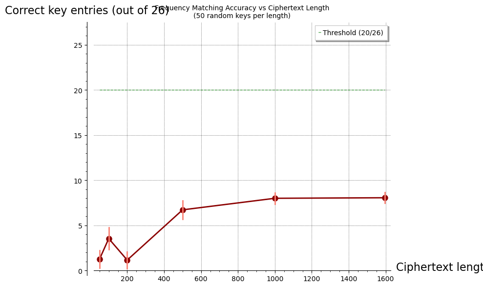
Results summary:
  Length    Mean correct     Std
--------------------------------
      50             1.3     1.0
     100             3.5     1.2
     200             1.2     0.9
     500             6.7     1.0
    1000             8.0     0.6
    1596             8.1     0.6

Summary

In this chapter we have studied the monoalphabetic substitution cipher – historically one of the most widely used cipher types – and the frequency-based methods that break it.

Key takeaways:

1. Monoalphabetic ciphers apply a single permutation \(\sigma \in S_{26}\) to every letter of the plaintext. Despite having a key space of size \(26! \approx 4 \times 10^{26}\), they are fatally vulnerable to statistical analysis.

2. Theorem 4.1 shows that a monoalphabetic cipher preserves digram structure: the digram frequency matrix of the ciphertext is a permuted version of the plaintext digram matrix. This extends to \(n\)-grams of any order.

3. The frequency matching attack (Algorithm 4.1) proceeds in stages:

   • Single-letter frequency matching gives a rough initial key.

   • Digram analysis refines ambiguous mappings.

   • Greedy swap improvement (or hill climbing) converges to the correct key.

4. The attack degrades gracefully with shorter ciphertext. Our experiments show that single-letter frequency matching alone becomes effective above roughly 200-500 characters; with digram refinement, shorter texts can also be attacked.

5. The asymmetry of English digrams (TH common, HT rare) provides particularly strong constraints on the key and is exploited by all practical attacks.

In the next chapter, we study the Vigen`ere cipher – a polyalphabetic system that was designed specifically to defeat the frequency analysis methods developed here – and the Kasiski examination that ultimately breaks it.

Broader Context: Classical Ciphers and Their Cryptanalysis

This chapter is part of a broader module on classical ciphers and their cryptanalysis. The techniques developed here – frequency analysis and digram matching – form the foundation for attacking more complex systems:

• Vigenere cipher: attack via index of coincidence and Kasiski method (Chapter 5–6)

• N-grams and hill climbing: efficient cryptanalysis of the general substitution cipher (Chapter 9)

• Playfair cipher: simulated annealing attack on a digram cipher (Chapter 8)

• Hill cipher: linear cryptanalysis of a matrix-based cipher (Chapter 7)

We explore probability-based methods of identifying connections in natural language:

• index of coincidence

• Kasiski examination

• n-grams analysis and fitness score

• hill climbing method

• simulated annealing

Literature

• U.S. Army Field Manual 34-40-2, Basic Cryptanalysis – an extensive source of information about classical ciphers and the methods of breaking them

References

1. Al-Kindi (c. 850 CE). A Manuscript on Deciphering Cryptographic Messages. Translated in: Al-Kadit, I. (1992). Origins of Cryptology: The Arab Contributions. Cryptologia, 16(2), 97–126.

2. Singh, S. (1999). The Code Book: The Science of Secrecy from Ancient Egypt to Quantum Cryptography. Fourth Estate. [Chapters 1–2 cover the history of monoalphabetic ciphers and the Mary Queen of Scots episode.]

3. Lewand, R. (2000). Cryptological Mathematics. MAA. [Standard reference for English letter and digram frequencies.]

4. US Army (1990). Field Manual 34-40-2: Basic Cryptanalysis. Department of the Army. [Systematic treatment of frequency analysis and manual cryptanalysis techniques.]

5. Stamp, M. and Low, R. (2007). Applied Cryptanalysis: Breaking Ciphers in the Real World. Wiley. [Chapter 2: Classical substitution ciphers and their cryptanalysis.]

6. Beker, H. and Piper, F. (1982). Cipher Systems: The Protection of Communications. Northwood. [Formal treatment of substitution ciphers and their properties.]