
Chapter 22: Finite Field Arithmetic in GF(2\(^8\))#
22.1 Introduction: Galois Fields and AES#
In 1830, the French mathematician Évariste Galois (1811–1832), in the last years of his tragically short life, laid the foundations of what we now call Galois theory. Among his discoveries was the complete classification of finite fields: for every prime \(p\) and positive integer \(n\), there exists a unique (up to isomorphism) finite field of order \(p^n\), denoted \(\mathrm{GF}(p^n)\) or \(\mathbb{F}_{p^n}\).
The field \(\mathrm{GF}(2^8)\) — a finite field with \(256\) elements — occupies a special place in modern cryptography. When Joan Daemen and Vincent Rijmen designed the Rijndael cipher in 1998 (which became the Advanced Encryption Standard in 2001), they chose \(\mathrm{GF}(2^8)\) as the algebraic foundation for nearly every operation in the cipher.
“The choice of \(\mathrm{GF}(2^8)\) as the basic algebraic structure was motivated by the fact that the elements of this field can be represented as bytes, making efficient software and hardware implementations possible.” — Daemen & Rijmen, The Design of Rijndael, 2002
Why \(\mathrm{GF}(2^8)\) specifically?
Byte representation. Each element of \(\mathrm{GF}(2^8)\) corresponds naturally to a single byte (8 bits), the fundamental unit of computation.
Efficient arithmetic. Addition in \(\mathrm{GF}(2^8)\) is simply XOR, which is one of the fastest operations on any processor.
Rich algebraic structure. Every nonzero element has a multiplicative inverse, enabling the construction of the AES S-box — the nonlinear component critical to the cipher’s security.
Hardware friendliness. Polynomial multiplication and reduction modulo a fixed polynomial can be implemented efficiently in both hardware and software.
The specific field used in AES is \(\mathrm{GF}(2^8)\) defined by the irreducible polynomial \(m(x) = x^8 + x^4 + x^3 + x + 1\) (hexadecimal 0x11B). This polynomial was chosen by the AES designers because it is the lexicographically first degree-8 irreducible polynomial over \(\mathrm{GF}(2)\) and produces an efficient reduction step.
Tip
Understanding \(\mathrm{GF}(2^8)\) arithmetic is essential for understanding AES at a mathematical level. The SubBytes step uses multiplicative inverses in this field, MixColumns uses polynomial multiplication over \(\mathrm{GF}(2^8)\), and AddRoundKey is simply addition (XOR) in the field.
22.2 Formal Definitions#
Definition 22.1 (The Binary Field \(\mathrm{GF}(2)\))
The binary field \(\mathrm{GF}(2) = \{0, 1\}\) is the finite field with two elements, where both addition and multiplication are performed modulo 2:
\(+\) |
0 |
1 |
|---|---|---|
0 |
0 |
1 |
1 |
1 |
0 |
\(\cdot\) |
0 |
1 |
|---|---|---|
0 |
0 |
0 |
1 |
0 |
1 |
Note that addition in \(\mathrm{GF}(2)\) is the XOR operation, and subtraction is identical to addition (since \(-1 \equiv 1 \pmod{2}\)).
Definition 22.2 (Polynomial Ring \(\mathrm{GF}(2)[x]\))
The polynomial ring \(\mathrm{GF}(2)[x]\) is the set of all polynomials with coefficients in \(\mathrm{GF}(2)\):
Addition and multiplication follow the usual polynomial rules, with all coefficient arithmetic done modulo 2. For example:
since \(1 + 1 = 0\) in \(\mathrm{GF}(2)\).
Definition 22.3 (The Finite Field \(\mathrm{GF}(2^8)\))
Let \(m(x) = x^8 + x^4 + x^3 + x + 1\) be an irreducible polynomial over \(\mathrm{GF}(2)\) (it has no nontrivial factors in \(\mathrm{GF}(2)[x]\)). The finite field \(\mathrm{GF}(2^8)\) is the quotient ring:
Its elements are the 256 polynomials of degree \(< 8\) over \(\mathrm{GF}(2)\):
Each element corresponds to a byte \((a_7, a_6, \ldots, a_1, a_0)\), or equivalently an integer in \(\{0, 1, \ldots, 255\}\).
Definition 22.4 (Addition in \(\mathrm{GF}(2^8)\))
Addition in \(\mathrm{GF}(2^8)\) is coefficient-wise addition modulo 2, which is equivalent to the bitwise XOR operation:
For example, 0x57 \(+\) 0x83 \(=\) 0xD4, since \(01010111 \oplus 10000011 = 11010100\).
Definition 22.5 (Multiplication in \(\mathrm{GF}(2^8)\))
Multiplication in \(\mathrm{GF}(2^8)\) is polynomial multiplication followed by reduction modulo \(m(x)\):
The reduction ensures the result is a polynomial of degree \(\leq 7\) (a single byte). For example, \(\{57\} \cdot \{83\} = \{\mathrm{C1}\}\) in the AES field.
Definition 22.6 (Multiplicative Inverse via Extended Euclidean Algorithm)
For a nonzero element \(a(x) \in \mathrm{GF}(2^8)\), its multiplicative inverse \(a^{-1}(x)\) satisfies:
It is computed using the extended Euclidean algorithm for polynomials over \(\mathrm{GF}(2)\). Since \(m(x)\) is irreducible and \(\deg(a) < \deg(m)\), we have \(\gcd(a(x), m(x)) = 1\), so Bézout’s identity gives:
and \(a^{-1}(x) = s(x) \mod m(x)\).
Theorem 22.1 (Existence of Multiplicative Inverses)
Every nonzero element of \(\mathrm{GF}(2^8)\) has a unique multiplicative inverse. Equivalently, \((\mathrm{GF}(2^8) \setminus \{0\}, \cdot)\) is a cyclic group of order 255.
Proof
Since \(m(x)\) is irreducible over \(\mathrm{GF}(2)\), the quotient ring \(\mathrm{GF}(2)[x]/(m(x))\) is a field. In any field, every nonzero element has a unique multiplicative inverse. Explicitly, for \(a(x) \neq 0\) with \(\deg(a) < 8\), the polynomials \(a(x)\) and \(m(x)\) share no common factor (since \(m(x)\) is irreducible and does not divide \(a(x)\)), so \(\gcd(a(x), m(x)) = 1\). By the extended Euclidean algorithm, there exist \(s(x), t(x)\) with \(s(x) \cdot a(x) + t(x) \cdot m(x) = 1\). Reducing modulo \(m(x)\): \(s(x) \cdot a(x) \equiv 1 \pmod{m(x)}\). Uniqueness follows from the cancellation law in fields. \(\blacksquare\)
Danger
The element \(0\) has no multiplicative inverse in any field. In the AES S-box, the input \(0\) is mapped to \(0\) before the affine transformation is applied. This is a special-case convention, not a field-theoretic operation.
22.3 Implementation: The GF256 Class#
We implement \(\mathrm{GF}(2^8)\) arithmetic using NumPy. Elements are represented as integers \(0\)–\(255\), corresponding to the coefficients of polynomials of degree \(\leq 7\) stored as bits.
import numpy as np
import matplotlib.pyplot as plt


class GF256:
    """
    Arithmetic in GF(2^8) = GF(2)[x] / (x^8 + x^4 + x^3 + x + 1).

    Elements are represented as integers 0-255.  Bit k of the integer
    corresponds to the coefficient of x^k in the polynomial representation.

    The irreducible (reducing) polynomial is m(x) = x^8+x^4+x^3+x+1 = 0x11B.
    """

    MODULUS = 0x11B          # x^8 + x^4 + x^3 + x + 1
    FIELD_ORDER = 256        # 2^8
    GROUP_ORDER = 255        # multiplicative group order

    # ----- core arithmetic -----

    @staticmethod
    def add(a, b):
        """Addition in GF(2^8) — bitwise XOR."""
        return a ^ b

    @staticmethod
    def multiply(a, b):
        """
        Multiplication in GF(2^8) via shift-and-XOR (Russian peasant method).

        Multiplies polynomials a(x)*b(x) and reduces modulo m(x).
        """
        result = 0
        a = a & 0xFF
        b = b & 0xFF
        for _ in range(8):
            if b & 1:                      # if lowest bit of b is set
                result ^= a                # add a(x) to result
            carry = a & 0x80               # check if a(x) has degree 7
            a = (a << 1) & 0xFF            # multiply a(x) by x
            if carry:                      # if degree overflowed to 8
                a ^= GF256.MODULUS & 0xFF  # reduce: subtract m(x)
            b >>= 1                        # next bit of b
        return result

    @staticmethod
    def _poly_degree(a):
        """Return the degree of the polynomial a (as an integer with bit-coefficients)."""
        if a == 0:
            return -1
        return a.bit_length() - 1

    @staticmethod
    def _poly_mod(a, m):
        """Reduce polynomial a modulo polynomial m (both as integers)."""
        deg_m = GF256._poly_degree(m)
        while True:
            deg_a = GF256._poly_degree(a)
            if deg_a < deg_m:
                return a
            a ^= m << (deg_a - deg_m)

    @staticmethod
    def _poly_divmod(a, b):
        """Polynomial division with remainder over GF(2).  Returns (quotient, remainder)."""
        if b == 0:
            raise ZeroDivisionError("Division by zero polynomial")
        q = 0
        deg_b = GF256._poly_degree(b)
        while True:
            deg_a = GF256._poly_degree(a)
            if deg_a < deg_b:
                return q, a
            shift = deg_a - deg_b
            q ^= 1 << shift
            a ^= b << shift

    @staticmethod
    def inverse(a):
        """
        Multiplicative inverse in GF(2^8) via the extended Euclidean algorithm
        for polynomials over GF(2).

        Returns a^{-1} such that  a * a^{-1} = 1  in GF(2^8).
        Raises ValueError if a == 0.
        """
        if a == 0:
            raise ValueError("Zero has no multiplicative inverse")

        r0, r1 = GF256.MODULUS, a
        s0, s1 = 0, 1

        while r1 != 0:
            q, r2 = GF256._poly_divmod(r0, r1)
            # s_new = s0 XOR q*s1  (polynomial multiplication over GF(2))
            s2 = s0 ^ GF256._poly_mul_full(q, s1)
            r0, r1 = r1, r2
            s0, s1 = s1, s2

        # r0 should be 1 (since m(x) is irreducible and a != 0)
        return s0 & 0xFF

    @staticmethod
    def _poly_mul_full(a, b):
        """Full polynomial multiplication over GF(2) (no reduction)."""
        result = 0
        while b:
            if b & 1:
                result ^= a
            a <<= 1
            b >>= 1
        return result

    @staticmethod
    def power(a, n):
        """Exponentiation in GF(2^8) via square-and-multiply."""
        if n == 0:
            return 1
        if n < 0:
            a = GF256.inverse(a)
            n = -n
        result = 1
        base = a & 0xFF
        while n > 0:
            if n & 1:
                result = GF256.multiply(result, base)
            base = GF256.multiply(base, base)
            n >>= 1
        return result

    @staticmethod
    def log_table(generator=0x03):
        """
        Build discrete-logarithm table:  log[a] = k  where  g^k = a.

        Parameters
        ----------
        generator : int
            A primitive element (generator) of GF(2^8)*.  Default is 0x03.

        Returns
        -------
        log_tbl : np.ndarray of shape (256,)
            log_tbl[0] is set to -1 (undefined).
        """
        log_tbl = np.full(256, -1, dtype=np.int16)
        val = 1
        for k in range(255):
            log_tbl[val] = k
            val = GF256.multiply(val, generator)
        return log_tbl

    @staticmethod
    def exp_table(generator=0x03):
        """
        Build antilog (exponentiation) table:  exp[k] = g^k.

        Returns
        -------
        exp_tbl : np.ndarray of shape (510,)
            Doubled to avoid modular reduction during multiplication.
        """
        exp_tbl = np.zeros(510, dtype=np.int16)
        val = 1
        for k in range(255):
            exp_tbl[k] = val
            exp_tbl[k + 255] = val   # wrap-around copy
            val = GF256.multiply(val, generator)
        return exp_tbl

    @staticmethod
    def build_mul_table():
        """Build the full 256x256 multiplication table."""
        tbl = np.zeros((256, 256), dtype=np.uint8)
        for a in range(256):
            for b in range(a, 256):
                p = GF256.multiply(a, b)
                tbl[a, b] = p
                tbl[b, a] = p
        return tbl

    @staticmethod
    def build_inv_table():
        """Build the complete inverse table (inv_tbl[a] = a^{-1})."""
        inv_tbl = np.zeros(256, dtype=np.uint8)
        for a in range(1, 256):
            inv_tbl[a] = GF256.inverse(a)
        return inv_tbl

    # ----- display helpers -----

    @staticmethod
    def to_poly_str(a):
        """Return a human-readable polynomial string for element a."""
        if a == 0:
            return "0"
        terms = []
        for k in range(7, -1, -1):
            if a & (1 << k):
                if k == 0:
                    terms.append("1")
                elif k == 1:
                    terms.append("x")
                else:
                    terms.append(f"x^{k}")
        return " + ".join(terms)

    @staticmethod
    def to_hex(a):
        """Return a two-character uppercase hex string."""
        return f"{a:02X}"


# --- Quick sanity checks ---
print("GF(2^8) with m(x) =", GF256.to_poly_str(GF256.MODULUS))
print(f"0x57 * 0x83 = 0x{GF256.multiply(0x57, 0x83):02X}")
print(f"0x57 + 0x83 = 0x{GF256.add(0x57, 0x83):02X}")
print(f"inverse(0x09) = 0x{GF256.inverse(0x09):02X}")
print(f"0x09 * inverse(0x09) = 0x{GF256.multiply(0x09, GF256.inverse(0x09)):02X}")
GF(2^8) with m(x) = x^4 + x^3 + x + 1
0x57 * 0x83 = 0xC1
0x57 + 0x83 = 0xD4
inverse(0x09) = 0x4F
0x09 * inverse(0x09) = 0x01
Let us verify the multiplication examples from the AES specification (FIPS 197, Section 4.2).
import numpy as np

# AES specification test vectors
test_cases = [
    (0x57, 0x83, 0xC1),
    (0x57, 0x13, 0xFE),
    (0x17, 0xA3, 0x9A),
]

print("Verifying AES spec multiplication examples:")
print("-" * 50)
for a, b, expected in test_cases:
    result = GF256.multiply(a, b)
    status = "PASS" if result == expected else "FAIL"
    print(f"  {GF256.to_hex(a)} * {GF256.to_hex(b)} = {GF256.to_hex(result)}  "
          f"(expected {GF256.to_hex(expected)})  [{status}]")

# Verify some inverses
print("\nVerifying inverses:")
print("-" * 50)
for a in [0x09, 0x27, 0x03, 0xFF]:
    a_inv = GF256.inverse(a)
    check = GF256.multiply(a, a_inv)
    print(f"  inverse({GF256.to_hex(a)}) = {GF256.to_hex(a_inv)}  "
          f"  verify: {GF256.to_hex(a)} * {GF256.to_hex(a_inv)} = {GF256.to_hex(check)}")

# Power examples
print("\nVerifying exponentiation:")
print("-" * 50)
for a, n, expected in [(0xF7, 6, 0xC3), (0x12, 6, 0x3B)]:
    result = GF256.power(a, n)
    status = "PASS" if result == expected else "FAIL"
    print(f"  {GF256.to_hex(a)}^{n} = {GF256.to_hex(result)}  "
          f"(expected {GF256.to_hex(expected)})  [{status}]")
Verifying AES spec multiplication examples:
--------------------------------------------------
  57 * 83 = C1  (expected C1)  [PASS]
  57 * 13 = FE  (expected FE)  [PASS]
  17 * A3 = 9A  (expected 9A)  [PASS]

Verifying inverses:
--------------------------------------------------
  inverse(09) = 4F    verify: 09 * 4F = 01
  inverse(27) = C9    verify: 27 * C9 = 01
  inverse(03) = F6    verify: 03 * F6 = 01
  inverse(FF) = 1C    verify: FF * 1C = 01

Verifying exponentiation:
--------------------------------------------------
  F7^6 = C3  (expected C3)  [PASS]
  12^6 = 3B  (expected 3B)  [PASS]
Polynomial representation#
Let us examine how bytes map to polynomials and trace through an addition and multiplication step by step.
import numpy as np

# Show the polynomial representation of several byte values
examples = [0x00, 0x01, 0x02, 0x03, 0x53, 0x57, 0x83, 0xCA, 0xFF]

print("Byte-to-polynomial correspondence:")
print("=" * 60)
for val in examples:
    bits = f"{val:08b}"
    print(f"  0x{val:02X}  =  {bits}  =  {GF256.to_poly_str(val)}")

print("\n--- Step-by-step addition ---")
a, b = 0x57, 0x83
print(f"  a = 0x{a:02X} = {a:08b} = {GF256.to_poly_str(a)}")
print(f"  b = 0x{b:02X} = {b:08b} = {GF256.to_poly_str(b)}")
s = GF256.add(a, b)
print(f"  a + b = {a:08b} XOR {b:08b} = {s:08b} = 0x{s:02X}")
print(f"        = {GF256.to_poly_str(s)}")

print("\n--- Step-by-step multiplication ---")
a, b = 0x57, 0x83
print(f"  a = {GF256.to_poly_str(a)}")
print(f"  b = {GF256.to_poly_str(b)}")
print(f"  m(x) = {GF256.to_poly_str(GF256.MODULUS)}")
# Full (unreduced) product
full = GF256._poly_mul_full(a, b)
print(f"  a(x)*b(x) = {GF256.to_poly_str(full)}  (degree {GF256._poly_degree(full)})")
reduced = GF256._poly_mod(full, GF256.MODULUS)
print(f"  reduced mod m(x) = {GF256.to_poly_str(reduced)} = 0x{reduced:02X}")
Byte-to-polynomial correspondence:
============================================================
  0x00  =  00000000  =  0
  0x01  =  00000001  =  1
  0x02  =  00000010  =  x
  0x03  =  00000011  =  x + 1
  0x53  =  01010011  =  x^6 + x^4 + x + 1
  0x57  =  01010111  =  x^6 + x^4 + x^2 + x + 1
  0x83  =  10000011  =  x^7 + x + 1
  0xCA  =  11001010  =  x^7 + x^6 + x^3 + x
  0xFF  =  11111111  =  x^7 + x^6 + x^5 + x^4 + x^3 + x^2 + x + 1

--- Step-by-step addition ---
  a = 0x57 = 01010111 = x^6 + x^4 + x^2 + x + 1
  b = 0x83 = 10000011 = x^7 + x + 1
  a + b = 01010111 XOR 10000011 = 11010100 = 0xD4
        = x^7 + x^6 + x^4 + x^2

--- Step-by-step multiplication ---
  a = x^6 + x^4 + x^2 + x + 1
  b = x^7 + x + 1
  m(x) = x^4 + x^3 + x + 1
  a(x)*b(x) = x^6 + x^5 + x^4 + x^3 + 1  (degree 13)
  reduced mod m(x) = x^7 + x^6 + 1 = 0xC1
Building complete lookup tables#
We precompute the log and exp (antilog) tables using the generator \(g = \mathtt{0x03}\) (corresponding to \(x + 1\)). Since \(g\) is a primitive element of \(\mathrm{GF}(2^8)^*\), it generates all 255 nonzero elements by repeated multiplication.
import numpy as np

# Build tables
log_tbl = GF256.log_table(generator=0x03)
exp_tbl = GF256.exp_table(generator=0x03)
inv_tbl = GF256.build_inv_table()

# Verify generator 0x03 is primitive (generates all 255 nonzero elements)
generated = set()
val = 1
for _ in range(255):
    generated.add(val)
    val = GF256.multiply(val, 0x03)
print(f"Generator 0x03 produces {len(generated)} distinct nonzero elements.")
assert len(generated) == 255, "0x03 is not a generator!"

# Display first 32 entries of the exp table
print("\nExponentiation table (0x03^k for k = 0..31):")
print("-" * 70)
for row_start in range(0, 32, 8):
    entries = [f"{int(exp_tbl[k]):3d} (0x{exp_tbl[k]:02X})" for k in range(row_start, row_start + 8)]
    labels = [f"g^{k:<2d}" for k in range(row_start, row_start + 8)]
    print("  " + "  ".join(f"{labels[i]}={entries[i]}" for i in range(8)))

# Display first 16 inverses
print("\nInverse table (first 16 nonzero elements):")
print("-" * 50)
for a in range(1, 17):
    a_inv = inv_tbl[a]
    print(f"  {GF256.to_hex(a)}^(-1) = {GF256.to_hex(a_inv)}  "
          f"  check: {GF256.to_hex(a)} * {GF256.to_hex(a_inv)} = "
          f"{GF256.to_hex(GF256.multiply(a, a_inv))}")
Generator 0x03 produces 255 distinct nonzero elements.

Exponentiation table (0x03^k for k = 0..31):
----------------------------------------------------------------------
  g^0 =  1 (0x01)  g^1 =  3 (0x03)  g^2 =  5 (0x05)  g^3 = 15 (0x0F)  g^4 = 17 (0x11)  g^5 = 51 (0x33)  g^6 = 85 (0x55)  g^7 =255 (0xFF)
  g^8 = 26 (0x1A)  g^9 = 46 (0x2E)  g^10=114 (0x72)  g^11=150 (0x96)  g^12=161 (0xA1)  g^13=248 (0xF8)  g^14= 19 (0x13)  g^15= 53 (0x35)
  g^16= 95 (0x5F)  g^17=225 (0xE1)  g^18= 56 (0x38)  g^19= 72 (0x48)  g^20=216 (0xD8)  g^21=115 (0x73)  g^22=149 (0x95)  g^23=164 (0xA4)
  g^24=247 (0xF7)  g^25=  2 (0x02)  g^26=  6 (0x06)  g^27= 10 (0x0A)  g^28= 30 (0x1E)  g^29= 34 (0x22)  g^30=102 (0x66)  g^31=170 (0xAA)

Inverse table (first 16 nonzero elements):
--------------------------------------------------
  01^(-1) = 01    check: 01 * 01 = 01
  02^(-1) = 8D    check: 02 * 8D = 01
  03^(-1) = F6    check: 03 * F6 = 01
  04^(-1) = CB    check: 04 * CB = 01
  05^(-1) = 52    check: 05 * 52 = 01
  06^(-1) = 7B    check: 06 * 7B = 01
  07^(-1) = D1    check: 07 * D1 = 01
  08^(-1) = E8    check: 08 * E8 = 01
  09^(-1) = 4F    check: 09 * 4F = 01
  0A^(-1) = 29    check: 0A * 29 = 01
  0B^(-1) = C0    check: 0B * C0 = 01
  0C^(-1) = B0    check: 0C * B0 = 01
  0D^(-1) = E1    check: 0D * E1 = 01
  0E^(-1) = E5    check: 0E * E5 = 01
  0F^(-1) = C7    check: 0F * C7 = 01
  10^(-1) = 74    check: 10 * 74 = 01
22.4 Experiments#
Experiment 1: Multiplication Table#
Heatmap
The full \(256 \times 256\) multiplication table of \(\mathrm{GF}(2^8)\) reveals the rich algebraic structure of the field. Unlike multiplication modulo \(n\) (which shows diagonal bands), the GF multiplication table has a pseudo-random, diffused appearance — precisely the property AES exploits for diffusion.
Show code cell source
import numpy as np
import matplotlib.pyplot as plt

mul_table = GF256.build_mul_table()

fig, axes = plt.subplots(1, 2, figsize=(14, 6))

# GF(2^8) multiplication table
im0 = axes[0].imshow(mul_table, cmap='inferno', aspect='equal', origin='lower')
axes[0].set_title('Multiplication table in GF($2^8$)', fontsize=13, fontweight='bold')
axes[0].set_xlabel('b', fontsize=11)
axes[0].set_ylabel('a', fontsize=11)
plt.colorbar(im0, ax=axes[0], fraction=0.046, pad=0.04, label='a * b')

# Compare: ordinary multiplication mod 256
ord_table = np.zeros((256, 256), dtype=np.uint8)
for i in range(256):
    for j in range(256):
        ord_table[i, j] = (i * j) % 256

im1 = axes[1].imshow(ord_table, cmap='inferno', aspect='equal', origin='lower')
axes[1].set_title('Ordinary multiplication mod 256', fontsize=13, fontweight='bold')
axes[1].set_xlabel('b', fontsize=11)
axes[1].set_ylabel('a', fontsize=11)
plt.colorbar(im1, ax=axes[1], fraction=0.046, pad=0.04, label='(a * b) mod 256')

plt.tight_layout()
plt.savefig('gf256_multiplication_heatmap.png', dpi=150, bbox_inches='tight')
plt.show()

print("Left: GF(2^8) multiplication — pseudo-random, excellent diffusion.")
print("Right: ordinary mod-256 multiplication — structured diagonal bands, poor diffusion.")
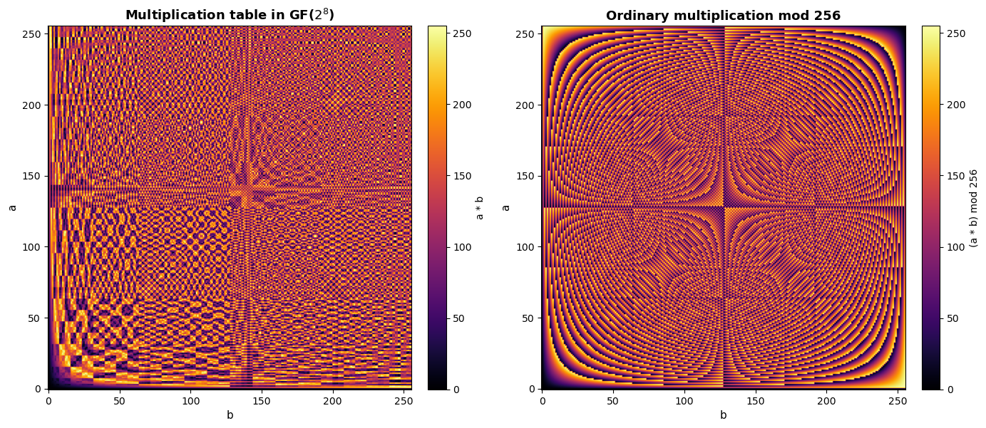
Left: GF(2^8) multiplication — pseudo-random, excellent diffusion.
Right: ordinary mod-256 multiplication — structured diagonal bands, poor diffusion.
Experiment 2: Verifying the Field Axioms#
A finite field must satisfy associativity, commutativity, distributivity, existence of identity elements, and existence of inverses. We verify these exhaustively (or on large random samples) for \(\mathrm{GF}(2^8)\).
import numpy as np

rng = np.random.default_rng(42)
N_TESTS = 50_000  # number of random triples to test

# Generate random triples
aa = rng.integers(0, 256, size=N_TESTS)
bb = rng.integers(0, 256, size=N_TESTS)
cc = rng.integers(0, 256, size=N_TESTS)

# Vectorised helpers (apply element-wise)
vmul = np.vectorize(GF256.multiply)
vadd = np.vectorize(GF256.add)

# 1. Commutativity of addition:  a + b == b + a
assert np.all(vadd(aa, bb) == vadd(bb, aa))
print("[PASS] Commutativity of addition    (a + b == b + a)")

# 2. Commutativity of multiplication:  a * b == b * a
assert np.all(vmul(aa, bb) == vmul(bb, aa))
print("[PASS] Commutativity of multiplication  (a * b == b * a)")

# 3. Associativity of addition:  (a + b) + c == a + (b + c)
lhs_add = vadd(vadd(aa, bb), cc)
rhs_add = vadd(aa, vadd(bb, cc))
assert np.all(lhs_add == rhs_add)
print("[PASS] Associativity of addition    ((a+b)+c == a+(b+c))")

# 4. Associativity of multiplication:  (a * b) * c == a * (b * c)
lhs_mul = vmul(vmul(aa, bb), cc)
rhs_mul = vmul(aa, vmul(bb, cc))
assert np.all(lhs_mul == rhs_mul)
print("[PASS] Associativity of multiplication  ((a*b)*c == a*(b*c))")

# 5. Distributivity:  a * (b + c) == a*b + a*c
lhs_dist = vmul(aa, vadd(bb, cc))
rhs_dist = vadd(vmul(aa, bb), vmul(aa, cc))
assert np.all(lhs_dist == rhs_dist)
print("[PASS] Distributivity               (a*(b+c) == a*b + a*c)")

# 6. Additive identity:  a + 0 == a
assert np.all(vadd(aa, 0) == aa)
print("[PASS] Additive identity            (a + 0 == a)")

# 7. Multiplicative identity:  a * 1 == a
assert np.all(vmul(aa, 1) == aa)
print("[PASS] Multiplicative identity      (a * 1 == a)")

# 8. Additive inverse:  a + a == 0  (in GF(2^n), every element is its own additive inverse)
assert np.all(vadd(aa, aa) == 0)
print("[PASS] Additive inverse             (a + a == 0)")

# 9. Multiplicative inverse (exhaustive for all 255 nonzero elements)
all_pass = True
for a in range(1, 256):
    a_inv = GF256.inverse(a)
    if GF256.multiply(a, a_inv) != 1:
        all_pass = False
        break
assert all_pass
print("[PASS] Multiplicative inverse       (a * a^{-1} == 1 for all a != 0)")

print(f"\nAll field axioms verified on {N_TESTS:,} random samples (and exhaustive inverses).")
[PASS] Commutativity of addition    (a + b == b + a)
[PASS] Commutativity of multiplication  (a * b == b * a)
[PASS] Associativity of addition    ((a+b)+c == a+(b+c))
[PASS] Associativity of multiplication  ((a*b)*c == a*(b*c))
[PASS] Distributivity               (a*(b+c) == a*b + a*c)
[PASS] Additive identity            (a + 0 == a)
[PASS] Multiplicative identity      (a * 1 == a)
[PASS] Additive inverse             (a + a == 0)
[PASS] Multiplicative inverse       (a * a^{-1} == 1 for all a != 0)

All field axioms verified on 50,000 random samples (and exhaustive inverses).
Experiment 3: Discrete Logarithm Function#
The discrete logarithm maps each nonzero element \(a \in \mathrm{GF}(2^8)^*\) to the unique exponent \(k\) such that \(g^k = a\), where \(g = \mathtt{0x03}\) is a primitive element. The apparent randomness of this mapping is fundamental to the security of logarithm-based cryptographic constructions.
Show code cell source
import numpy as np
import matplotlib.pyplot as plt

log_tbl = GF256.log_table(generator=0x03)
exp_tbl = GF256.exp_table(generator=0x03)

fig, axes = plt.subplots(1, 2, figsize=(14, 5))

# Plot 1: Discrete log  (a -> log_g(a))
x_vals = np.arange(1, 256)
y_vals = log_tbl[1:256]
axes[0].scatter(x_vals, y_vals, s=3, c=y_vals, cmap='viridis', alpha=0.8)
axes[0].set_xlabel('Element a (integer representation)', fontsize=11)
axes[0].set_ylabel('$\\log_{g}(a)$', fontsize=11)
axes[0].set_title('Discrete logarithm in GF($2^8$)', fontsize=13, fontweight='bold')
axes[0].set_xlim(0, 256)
axes[0].set_ylim(-5, 260)
axes[0].grid(alpha=0.3)

# Plot 2: Exponential  (k -> g^k)
k_vals = np.arange(0, 255)
e_vals = exp_tbl[:255]
axes[1].scatter(k_vals, e_vals, s=3, c=k_vals, cmap='plasma', alpha=0.8)
axes[1].set_xlabel('Exponent k', fontsize=11)
axes[1].set_ylabel('$g^k$', fontsize=11)
axes[1].set_title('Exponentiation $g^k$ in GF($2^8$) ($g$ = 0x03)', fontsize=13, fontweight='bold')
axes[1].set_xlim(-5, 260)
axes[1].set_ylim(0, 260)
axes[1].grid(alpha=0.3)

plt.tight_layout()
plt.savefig('gf256_discrete_log.png', dpi=150, bbox_inches='tight')
plt.show()

print("The discrete logarithm appears as a pseudo-random permutation of {0,...,254}.")
print("This 'randomness' is what makes discrete-log-based cryptography hard.")
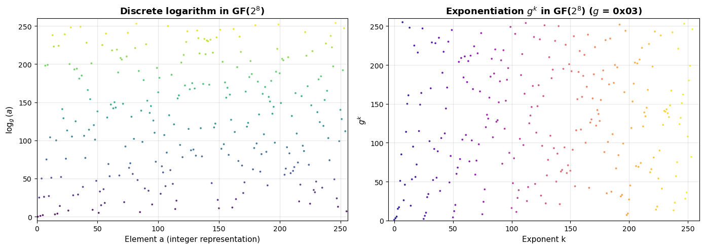
The discrete logarithm appears as a pseudo-random permutation of {0,...,254}.
This 'randomness' is what makes discrete-log-based cryptography hard.
Experiment 4: Multiplication via Log/Antilog Tables#
Once the log and antilog (exp) tables are precomputed, multiplication in \(\mathrm{GF}(2^8)\) reduces to:
This replaces an \(O(n^2)\) polynomial multiplication with three table lookups and one addition — a significant speedup, especially in hardware.
import numpy as np
import matplotlib.pyplot as plt

log_tbl = GF256.log_table(generator=0x03)
exp_tbl = GF256.exp_table(generator=0x03)


def multiply_via_tables(a, b, log_t, exp_t):
    """Multiply in GF(2^8) using log/antilog tables."""
    if a == 0 or b == 0:
        return 0
    log_sum = int(log_t[a]) + int(log_t[b])  # may exceed 254
    return int(exp_t[log_sum])                # exp table is doubled to handle this


# Verify: compare table-based multiplication against direct multiplication
print("Comparing schoolbook vs. log/antilog multiplication:")
print("=" * 55)
mismatches = 0
for a in range(256):
    for b in range(256):
        direct = GF256.multiply(a, b)
        table = multiply_via_tables(a, b, log_tbl, exp_tbl)
        if direct != table:
            mismatches += 1

print(f"  Tested all 256 x 256 = 65536 products.")
print(f"  Mismatches: {mismatches}")
print(f"  Result: {'PASS — methods agree perfectly' if mismatches == 0 else 'FAIL'}")

# Timing comparison
import time

rng = np.random.default_rng(123)
test_a = rng.integers(1, 256, size=100_000)
test_b = rng.integers(1, 256, size=100_000)

# Schoolbook
t0 = time.perf_counter()
for i in range(len(test_a)):
    GF256.multiply(int(test_a[i]), int(test_b[i]))
t_schoolbook = time.perf_counter() - t0

# Table-based
t0 = time.perf_counter()
for i in range(len(test_a)):
    multiply_via_tables(int(test_a[i]), int(test_b[i]), log_tbl, exp_tbl)
t_table = time.perf_counter() - t0

print(f"\nTiming ({len(test_a):,} multiplications):")
print(f"  Schoolbook (shift-and-XOR): {float(t_schoolbook):.3f} s")
print(f"  Log/antilog table lookup:   {float(t_table):.3f} s")
print(f"  Speedup factor:             {float(t_schoolbook / t_table):.2f}x")
Comparing schoolbook vs. log/antilog multiplication:
=======================================================
  Tested all 256 x 256 = 65536 products.
  Mismatches: 0
  Result: PASS — methods agree perfectly
Timing (100,000 multiplications):
  Schoolbook (shift-and-XOR): 0.123 s
  Log/antilog table lookup:   0.058 s
  Speedup factor:             2.14x
Experiment 5: Structure of the Multiplicative Group#
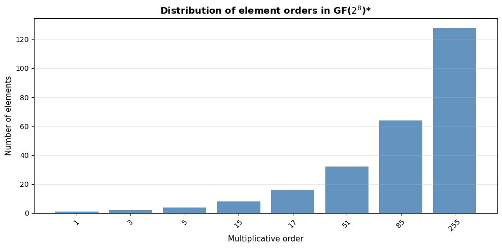
The multiplicative group \(\mathrm{GF}(2^8)^*\) is cyclic of order 255. Not every nonzero element is a generator. The order of an element \(a\) (the smallest \(k > 0\) with \(a^k = 1\)) must divide 255. Let us investigate the distribution of element orders and identify all generators.
Show code cell source
import numpy as np
import matplotlib.pyplot as plt


def element_order(a):
    """Compute the multiplicative order of a in GF(2^8)."""
    if a == 0:
        return 0
    val = a
    for k in range(1, 256):
        if val == 1:
            return k
        val = GF256.multiply(val, a)
    return -1  # should not happen


# Compute order of every nonzero element
orders = np.array([element_order(a) for a in range(256)])

# Divisors of 255 = 3 * 5 * 17
divisors_255 = sorted([d for d in range(1, 256) if 255 % d == 0])
print(f"255 = 3 x 5 x 17")
print(f"Divisors of 255: {divisors_255}")
print(f"Number of divisors: {len(divisors_255)}")

# Count elements of each order
print(f"\n{'Order':>6s}  {'Count':>6s}  {'phi(order)':>10s}")
print("-" * 28)
for d in divisors_255:
    count = np.sum(orders[1:] == d)  # exclude 0
    # Euler totient for comparison
    phi = d
    for p in [3, 5, 17]:
        if d % p == 0:
            phi = phi * (p - 1) // p
    print(f"  {int(d):>4d}  {int(count):>6d}  {int(phi):>10d}")

generators = [a for a in range(1, 256) if orders[a] == 255]
print(f"\nNumber of generators (primitive elements): {len(generators)}")
print(f"Euler totient phi(255) = phi(3)*phi(5)*phi(17) = 2*4*16 = {2*4*16}")
print(f"First 10 generators: {[f'0x{g:02X}' for g in generators[:10]]}")

# Plot order distribution
fig, ax = plt.subplots(figsize=(10, 5))
order_counts = [(d, np.sum(orders[1:] == d)) for d in divisors_255]
x_pos = np.arange(len(divisors_255))
ax.bar(x_pos, [c for _, c in order_counts], color='steelblue', alpha=0.85)
ax.set_xticks(x_pos)
ax.set_xticklabels([str(d) for d in divisors_255], rotation=45)
ax.set_xlabel('Multiplicative order', fontsize=11)
ax.set_ylabel('Number of elements', fontsize=11)
ax.set_title('Distribution of element orders in GF($2^8$)*', fontsize=13, fontweight='bold')
ax.grid(axis='y', alpha=0.3)

plt.tight_layout()
plt.savefig('gf256_order_distribution.png', dpi=150, bbox_inches='tight')
plt.show()
255 = 3 x 5 x 17
Divisors of 255: [1, 3, 5, 15, 17, 51, 85, 255]
Number of divisors: 8

 Order   Count  phi(order)
----------------------------
     1       1           1
     3       2           2
     5       4           4
    15       8           8
    17      16          16
    51      32          32
    85      64          64
   255     128         128

Number of generators (primitive elements): 128
Euler totient phi(255) = phi(3)*phi(5)*phi(17) = 2*4*16 = 128
First 10 generators: ['0x03', '0x05', '0x06', '0x09', '0x0B', '0x0E', '0x11', '0x12', '0x13', '0x14']
Experiment 6: The AES Inverse Table and S-Box Connection#
The AES S-box is constructed from two components:
The multiplicative inverse in \(\mathrm{GF}(2^8)\) (with \(0 \mapsto 0\)).
An affine transformation over \(\mathrm{GF}(2)\).
Let us visualize the inverse map and understand why it provides excellent nonlinearity.
Show code cell source
import numpy as np
import matplotlib.pyplot as plt

inv_tbl = GF256.build_inv_table()

fig, axes = plt.subplots(1, 2, figsize=(14, 5))

# Plot 1: Inverse map  a -> a^{-1}
x_vals = np.arange(256)
axes[0].scatter(x_vals, inv_tbl, s=4, c=inv_tbl, cmap='coolwarm', alpha=0.8)
axes[0].set_xlabel('a', fontsize=11)
axes[0].set_ylabel('$a^{-1}$', fontsize=11)
axes[0].set_title('Multiplicative inverse in GF($2^8$)', fontsize=13, fontweight='bold')
axes[0].set_xlim(-5, 260)
axes[0].set_ylim(-5, 260)
axes[0].grid(alpha=0.3)

# Plot 2: Inverse as a 16x16 grid (byte value heatmap)
inv_grid = inv_tbl.reshape(16, 16)
im = axes[1].imshow(inv_grid, cmap='viridis', aspect='equal')
axes[1].set_xlabel('Low nibble', fontsize=11)
axes[1].set_ylabel('High nibble', fontsize=11)
axes[1].set_title('Inverse table as 16$\\times$16 grid', fontsize=13, fontweight='bold')
axes[1].set_xticks(range(16))
axes[1].set_xticklabels([f'{i:X}' for i in range(16)])
axes[1].set_yticks(range(16))
axes[1].set_yticklabels([f'{i:X}' for i in range(16)])
plt.colorbar(im, ax=axes[1], fraction=0.046, pad=0.04, label='$a^{-1}$')

plt.tight_layout()
plt.savefig('gf256_inverse_map.png', dpi=150, bbox_inches='tight')
plt.show()

# Verify involutory property: (a^{-1})^{-1} = a
double_inv = inv_tbl[inv_tbl]  # apply inverse twice
double_inv[0] = 0  # handle 0 -> 0 -> 0
assert np.all(double_inv == np.arange(256, dtype=np.uint8))
print("Verified: (a^{-1})^{-1} = a for all elements.")

# Fixed points: a = a^{-1} means a^2 = 1
fixed = [a for a in range(256) if inv_tbl[a] == a]
print(f"\nFixed points of the inverse map (a^2 = 1): {[f'0x{a:02X}' for a in fixed]}")
print(f"These are the square roots of unity in GF(2^8).")
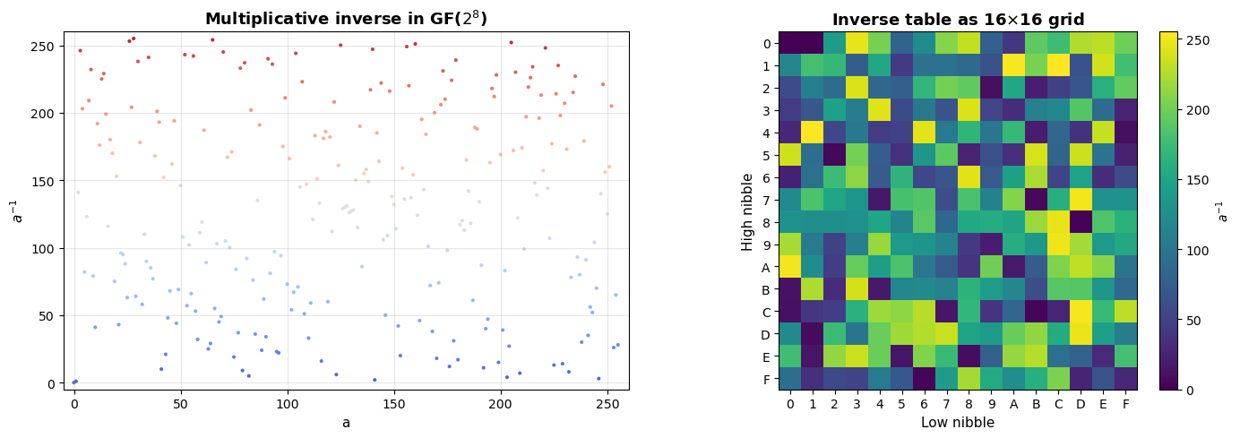
Verified: (a^{-1})^{-1} = a for all elements.

Fixed points of the inverse map (a^2 = 1): ['0x00', '0x01']
These are the square roots of unity in GF(2^8).
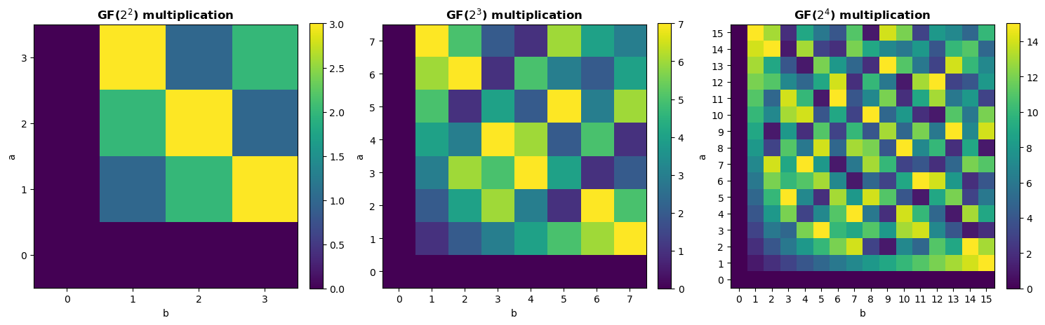
Experiment 7: Arithmetic in Small Extension Fields#
Before tackling \(\mathrm{GF}(2^8)\) in full, it is instructive to examine the smaller fields \(\mathrm{GF}(2^2)\), \(\mathrm{GF}(2^3)\), and \(\mathrm{GF}(2^4)\). These are small enough to display complete addition and multiplication tables.
Note on the element 0
0 is not a unit in GF(2^8), so it is excluded from the group of units. The convention inv(0) = 0 used in AES is a special case for implementation convenience.
Show code cell source
import numpy as np
import matplotlib.pyplot as plt


def gf_multiply(a, b, modulus):
    """Multiply two elements in GF(2^n) with given irreducible modulus."""
    result = 0
    while b:
        if b & 1:
            result ^= a
        a <<= 1
        b >>= 1
    # Reduce modulo the irreducible polynomial
    deg_m = modulus.bit_length() - 1
    while True:
        deg_r = result.bit_length() - 1
        if deg_r < deg_m:
            return result
        result ^= modulus << (deg_r - deg_m)


# Small fields: (name, modulus polynomial, field size)
small_fields = [
    ('GF($2^2$)', 0b111, 4),           # x^2 + x + 1
    ('GF($2^3$)', 0b1011, 8),          # x^3 + x + 1
    ('GF($2^4$)', 0b10011, 16),        # x^4 + x + 1
]

fig, axes = plt.subplots(1, 3, figsize=(15, 4.5))

for idx, (name, mod, size) in enumerate(small_fields):
    mul_tbl = np.zeros((size, size), dtype=int)
    for i in range(size):
        for j in range(size):
            mul_tbl[i, j] = gf_multiply(i, j, mod)

    im = axes[idx].imshow(mul_tbl, cmap='viridis', aspect='equal', origin='lower')
    axes[idx].set_title(f'{name} multiplication', fontsize=12, fontweight='bold')
    axes[idx].set_xlabel('b', fontsize=10)
    axes[idx].set_ylabel('a', fontsize=10)
    axes[idx].set_xticks(range(size))
    axes[idx].set_yticks(range(size))
    plt.colorbar(im, ax=axes[idx], fraction=0.046, pad=0.04)

plt.tight_layout()
plt.savefig('gf_small_fields.png', dpi=150, bbox_inches='tight')
plt.show()

# Print the full GF(2^2) tables
print("Complete multiplication table for GF(2^2) = GF(2)[x]/(x^2+x+1):")
print("Elements: 0, 1, x, x+1  (as integers: 0, 1, 2, 3)")
print()
labels = ['0', '1', 'x', 'x+1']
mod4 = 0b111
print(f"{'*':>5s}", end='')
for j in range(4):
    print(f"{labels[j]:>6s}", end='')
print()
print('-' * 29)
for i in range(4):
    print(f"{labels[i]:>5s}", end='')
    for j in range(4):
        r = gf_multiply(i, j, mod4)
        print(f"{labels[r]:>6s}", end='')
    print()
Complete multiplication table for GF(2^2) = GF(2)[x]/(x^2+x+1):
Elements: 0, 1, x, x+1  (as integers: 0, 1, 2, 3)

    *     0     1     x   x+1
-----------------------------
    0     0     0     0     0
    1     0     1     x   x+1
    x     0     x   x+1     1
  x+1     0   x+1     1     x
Experiment 8: Irreducible Polynomials of Degree 8 over GF(2)#
There are exactly 30 irreducible polynomials of degree 8 over \(\mathrm{GF}(2)\). Any of them could be used to construct \(\mathrm{GF}(2^8)\), producing isomorphic fields. The AES designers chose \(m(x) = x^8 + x^4 + x^3 + x + 1\) (the lexicographically first one with minimal nonzero terms after \(x^8\) and \(1\)). Let us enumerate all 30.
import numpy as np


def is_irreducible_gf2(poly):
    """
    Test if a polynomial over GF(2) is irreducible, by checking that
    it has no nontrivial factors of degree 1..floor(deg/2).
    """
    deg = poly.bit_length() - 1
    if deg <= 0:
        return False
    if deg == 1:
        return True

    # Check divisibility by all irreducible polynomials of degree <= deg//2
    # Efficient approach: check if poly divides x^(2^k) - x for k = 1..deg//2
    # but for degree 8, brute-force trial division is fast enough.

    # Generate all polynomials of degree 1..deg//2 and test
    for d in range(1, deg // 2 + 1):
        # All monic polynomials of degree d
        for lower_bits in range(1 << d):  # coefficients below leading term
            trial = (1 << d) | lower_bits
            _, rem = _divmod_gf2(poly, trial)
            if rem == 0:
                return False
    return True


def _divmod_gf2(a, b):
    """Polynomial division with remainder over GF(2)."""
    if b == 0:
        raise ZeroDivisionError
    q = 0
    deg_b = b.bit_length() - 1
    while True:
        deg_a = a.bit_length() - 1
        if deg_a < deg_b:
            return q, a
        shift = deg_a - deg_b
        q ^= 1 << shift
        a ^= b << shift


def poly_to_str(p):
    """Convert an integer-encoded GF(2) polynomial to a readable string."""
    if p == 0:
        return '0'
    terms = []
    for k in range(p.bit_length() - 1, -1, -1):
        if p & (1 << k):
            if k == 0:
                terms.append('1')
            elif k == 1:
                terms.append('x')
            else:
                terms.append(f'x^{k}')
    return ' + '.join(terms)


# Enumerate all monic degree-8 irreducible polynomials over GF(2)
# They have the form x^8 + (lower terms) + 1  (constant term must be 1 for irreducibility)
irred_deg8 = []
for lower in range(256):  # coefficients of x^0 through x^7
    poly = (1 << 8) | lower  # monic degree 8
    if not (poly & 1):       # constant term must be 1
        continue
    if is_irreducible_gf2(poly):
        irred_deg8.append(poly)

print(f"Number of irreducible degree-8 polynomials over GF(2): {len(irred_deg8)}")
print(f"\nAll {len(irred_deg8)} polynomials:")
print("=" * 60)
for i, p in enumerate(irred_deg8):
    marker = "  <-- AES" if p == 0x11B else ""
    print(f"  {int(i+1):2d}. 0x{p:03X}  =  {poly_to_str(p)}{marker}")

# Verify the count matches the formula:
# Number of monic irreducible polynomials of degree n over GF(q)
# = (1/n) * sum_{d|n} mu(n/d) * q^d
# For n=8, q=2: (1/8)(2^8 - 2^4) = (256 - 16)/8 = 30
print(f"\nFormula check: (2^8 - 2^4) / 8 = {(256 - 16) // 8}")
Number of irreducible degree-8 polynomials over GF(2): 30

All 30 polynomials:
============================================================
   1. 0x11B  =  x^8 + x^4 + x^3 + x + 1  <-- AES
   2. 0x11D  =  x^8 + x^4 + x^3 + x^2 + 1
   3. 0x12B  =  x^8 + x^5 + x^3 + x + 1
   4. 0x12D  =  x^8 + x^5 + x^3 + x^2 + 1
   5. 0x139  =  x^8 + x^5 + x^4 + x^3 + 1
   6. 0x13F  =  x^8 + x^5 + x^4 + x^3 + x^2 + x + 1
   7. 0x14D  =  x^8 + x^6 + x^3 + x^2 + 1
   8. 0x15F  =  x^8 + x^6 + x^4 + x^3 + x^2 + x + 1
   9. 0x163  =  x^8 + x^6 + x^5 + x + 1
  10. 0x165  =  x^8 + x^6 + x^5 + x^2 + 1
  11. 0x169  =  x^8 + x^6 + x^5 + x^3 + 1
  12. 0x171  =  x^8 + x^6 + x^5 + x^4 + 1
  13. 0x177  =  x^8 + x^6 + x^5 + x^4 + x^2 + x + 1
  14. 0x17B  =  x^8 + x^6 + x^5 + x^4 + x^3 + x + 1
  15. 0x187  =  x^8 + x^7 + x^2 + x + 1
  16. 0x18B  =  x^8 + x^7 + x^3 + x + 1
  17. 0x18D  =  x^8 + x^7 + x^3 + x^2 + 1
  18. 0x19F  =  x^8 + x^7 + x^4 + x^3 + x^2 + x + 1
  19. 0x1A3  =  x^8 + x^7 + x^5 + x + 1
  20. 0x1A9  =  x^8 + x^7 + x^5 + x^3 + 1
  21. 0x1B1  =  x^8 + x^7 + x^5 + x^4 + 1
  22. 0x1BD  =  x^8 + x^7 + x^5 + x^4 + x^3 + x^2 + 1
  23. 0x1C3  =  x^8 + x^7 + x^6 + x + 1
  24. 0x1CF  =  x^8 + x^7 + x^6 + x^3 + x^2 + x + 1
  25. 0x1D7  =  x^8 + x^7 + x^6 + x^4 + x^2 + x + 1
  26. 0x1DD  =  x^8 + x^7 + x^6 + x^4 + x^3 + x^2 + 1
  27. 0x1E7  =  x^8 + x^7 + x^6 + x^5 + x^2 + x + 1
  28. 0x1F3  =  x^8 + x^7 + x^6 + x^5 + x^4 + x + 1
  29. 0x1F5  =  x^8 + x^7 + x^6 + x^5 + x^4 + x^2 + 1
  30. 0x1F9  =  x^8 + x^7 + x^6 + x^5 + x^4 + x^3 + 1

Formula check: (2^8 - 2^4) / 8 = 30
Experiment 9: Visualizing the Extended Euclidean Algorithm#
The extended Euclidean algorithm for polynomials over \(\mathrm{GF}(2)\) is the heart of the inverse computation. Let us trace through a complete example.
import numpy as np


def extended_gcd_trace(a, modulus):
    """
    Extended Euclidean algorithm for polynomials over GF(2),
    with step-by-step trace.

    Computes s(x) such that s(x)*a(x) + t(x)*m(x) = 1.
    """
    r0, r1 = modulus, a
    s0, s1 = 0, 1
    t0, t1 = 1, 0
    step = 0

    print(f"Computing inverse of a(x) = {GF256.to_poly_str(a)} in GF(2^8)")
    print(f"Modulus m(x) = {GF256.to_poly_str(modulus)}")
    print("=" * 75)
    print(f"{'Step':>4s}  {'r(x)':>25s}  {'s(x)':>20s}  {'q(x)':>15s}")
    print("-" * 75)
    print(f"{'init':>4s}  r0 = {GF256.to_poly_str(r0):>20s}  s0 = {GF256.to_poly_str(s0):>15s}")
    print(f"{'':>4s}  r1 = {GF256.to_poly_str(r1):>20s}  s1 = {GF256.to_poly_str(s1):>15s}")

    while r1 != 0:
        step += 1
        q, r2 = GF256._poly_divmod(r0, r1)
        s2 = s0 ^ GF256._poly_mul_full(q, s1)
        t2 = t0 ^ GF256._poly_mul_full(q, t1)

        print(f"{int(step):>4d}  r{step+1} = {GF256.to_poly_str(r2):>20s}  "
              f"s{step+1} = {GF256.to_poly_str(s2):>15s}  "
              f"q = {GF256.to_poly_str(q):>12s}")

        r0, r1 = r1, r2
        s0, s1 = s1, s2
        t0, t1 = t1, t2

    print("-" * 75)
    print(f"GCD = {GF256.to_poly_str(r0)}")
    inverse = s0 & 0xFF
    print(f"Inverse: s(x) = {GF256.to_poly_str(inverse)} = 0x{inverse:02X}")

    # Verify
    check = GF256.multiply(a, inverse)
    print(f"Verify: a(x) * s(x) mod m(x) = {GF256.to_poly_str(check)} = 0x{check:02X}")
    return inverse


# Trace the inverse of 0x53 (used in AES S-box for input 0x53)
print("Example 1: inverse of 0x53")
inv_53 = extended_gcd_trace(0x53, GF256.MODULUS)

print("\n" + "=" * 75)
print("\nExample 2: inverse of 0x03 (the AES generator)")
inv_03 = extended_gcd_trace(0x03, GF256.MODULUS)
Example 1: inverse of 0x53
Computing inverse of a(x) = x^6 + x^4 + x + 1 in GF(2^8)
Modulus m(x) = x^4 + x^3 + x + 1
===========================================================================
Step                       r(x)                  s(x)             q(x)
---------------------------------------------------------------------------
init  r0 =    x^4 + x^3 + x + 1  s0 =               0
      r1 =    x^6 + x^4 + x + 1  s1 =               1
   1  r2 =                  x^2  s2 =         x^2 + 1  q =      x^2 + 1
   2  r3 =                x + 1  s3 =   x^6 + x^2 + 1  q =    x^4 + x^2
   3  r4 =                    1  s4 = x^7 + x^6 + x^3 + x  q =        x + 1
   4  r5 =                    0  s5 = x^4 + x^3 + x + 1  q =        x + 1
---------------------------------------------------------------------------
GCD = 1
Inverse: s(x) = x^7 + x^6 + x^3 + x = 0xCA
Verify: a(x) * s(x) mod m(x) = 1 = 0x01

===========================================================================

Example 2: inverse of 0x03 (the AES generator)
Computing inverse of a(x) = x + 1 in GF(2^8)
Modulus m(x) = x^4 + x^3 + x + 1
===========================================================================
Step                       r(x)                  s(x)             q(x)
---------------------------------------------------------------------------
init  r0 =    x^4 + x^3 + x + 1  s0 =               0
      r1 =                x + 1  s1 =               1
   1  r2 =                    1  s2 = x^7 + x^6 + x^5 + x^4 + x^2 + x  q = x^7 + x^6 + x^5 + x^4 + x^2 + x
   2  r3 =                    0  s3 = x^4 + x^3 + x + 1  q =        x + 1
---------------------------------------------------------------------------
GCD = 1
Inverse: s(x) = x^7 + x^6 + x^5 + x^4 + x^2 + x = 0xF6
Verify: a(x) * s(x) mod m(x) = 1 = 0x01
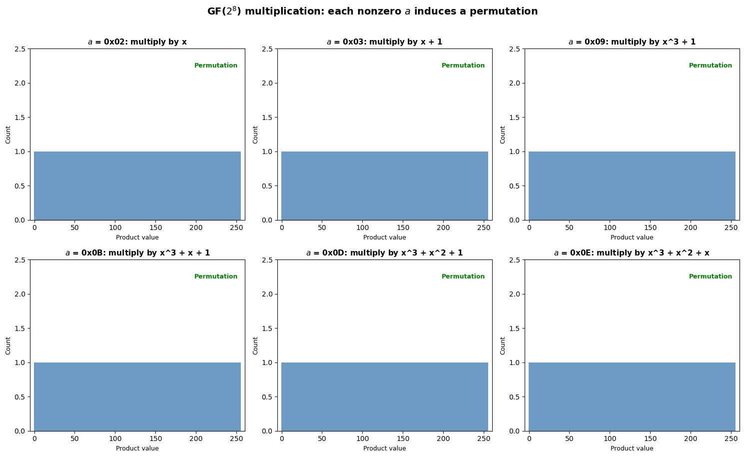
Experiment 10: Output Distribution of GF(2\(^8\)) Multiplication#
A key property of field multiplication (vs. ring multiplication modulo \(2^8\)) is that for any fixed nonzero \(a\), the map \(b \mapsto a \cdot b\) is a permutation of \(\mathrm{GF}(2^8)\). This is precisely what makes it useful for diffusion in AES MixColumns.
Show code cell source
import numpy as np
import matplotlib.pyplot as plt

# For several fixed values of a, compute {a*b : b in 0..255}
test_values = [0x02, 0x03, 0x09, 0x0B, 0x0D, 0x0E]  # values used in AES MixColumns

fig, axes = plt.subplots(2, 3, figsize=(15, 9))

for idx, a in enumerate(test_values):
    ax = axes[idx // 3, idx % 3]
    products = np.array([GF256.multiply(a, b) for b in range(256)])

    # Check permutation property
    is_perm = len(set(products)) == 256

    # Histogram of output values
    ax.hist(products, bins=np.arange(257) - 0.5, color='steelblue', alpha=0.8,
            edgecolor='none')
    ax.set_title(f'$a$ = 0x{a:02X}: multiply by {GF256.to_poly_str(a)}',
                 fontsize=11, fontweight='bold')
    ax.set_xlabel('Product value', fontsize=9)
    ax.set_ylabel('Count', fontsize=9)
    ax.set_xlim(-5, 260)
    ax.set_ylim(0, 2.5)
    perm_str = 'Permutation' if is_perm else 'NOT permutation'
    ax.text(0.97, 0.92, perm_str, transform=ax.transAxes,
            ha='right', va='top', fontsize=9,
            color='green' if is_perm else 'red', fontweight='bold')

plt.suptitle('GF($2^8$) multiplication: each nonzero $a$ induces a permutation',
             fontsize=14, fontweight='bold', y=1.01)
plt.tight_layout()
plt.savefig('gf256_permutation_property.png', dpi=150, bbox_inches='tight')
plt.show()

# Contrast with ordinary mod-256 multiplication
print("Contrast: ordinary multiplication mod 256")
print("-" * 50)
for a in [2, 3, 4, 6]:
    products_ord = set((a * b) % 256 for b in range(256))
    print(f"  a={a}: {len(products_ord)} distinct outputs out of 256"
          f"  ({'permutation' if len(products_ord) == 256 else 'NOT permutation'})")
Contrast: ordinary multiplication mod 256
--------------------------------------------------
  a=2: 128 distinct outputs out of 256  (NOT permutation)
  a=3: 256 distinct outputs out of 256  (permutation)
  a=4: 64 distinct outputs out of 256  (NOT permutation)
  a=6: 128 distinct outputs out of 256  (NOT permutation)
22.5 Exercises#
Exercise 22.1: Hand Computation#
Compute \(\{\mathtt{0xAB}\} \cdot \{\mathtt{0xCD}\}\) in \(\mathrm{GF}(2^8)\) by hand. Write out both polynomials, perform the full polynomial multiplication over \(\mathrm{GF}(2)\), and reduce modulo \(m(x) = x^8 + x^4 + x^3 + x + 1\).
Hint
\(\mathtt{0xAB} = x^7 + x^5 + x^3 + x + 1\) and \(\mathtt{0xCD} = x^7 + x^6 + x^3 + x^2 + 1\). Multiply term by term (remembering that \(1 + 1 = 0\) in \(\mathrm{GF}(2)\)), then reduce the degree-14 result modulo \(m(x)\) by repeatedly replacing \(x^8\) with \(x^4 + x^3 + x + 1\). The answer is \(\mathtt{0xAB} \cdot \mathtt{0xCD} = \mathtt{0x6B}\). Verify with GF256.multiply(0xAB, 0xCD).
Exercise 22.2: Proving Irreducibility#
Prove that \(m(x) = x^8 + x^4 + x^3 + x + 1\) is irreducible over \(\mathrm{GF}(2)\). How many candidate divisors must you check?
Hint
A degree-8 polynomial is irreducible iff it has no irreducible factors of degree 1, 2, 3, or 4. There is 1 irreducible of degree 1 (\(x + 1\)), 1 of degree 2 (\(x^2 + x + 1\)), 2 of degree 3, and 3 of degree 4 — a total of 7 trial divisions. Check that none of them divide \(m(x)\). Alternatively, verify that \(\gcd(m(x), x^{2^k} + x) = 1\) for \(k = 1, 2, 3, 4\).
Exercise 22.3: Subfield Structure#
Show that \(\mathrm{GF}(2^8)\) contains exactly one copy of \(\mathrm{GF}(2^2)\) and one copy of \(\mathrm{GF}(2^4)\) as subfields. Find the elements of each subfield explicitly.
Hint
The subfields of \(\mathrm{GF}(2^n)\) correspond to the divisors \(d\) of \(n\). For \(n = 8\): \(d \in \{1, 2, 4, 8\}\), giving subfields \(\mathrm{GF}(2)\), \(\mathrm{GF}(2^2)\), \(\mathrm{GF}(2^4)\), and \(\mathrm{GF}(2^8)\) itself. The elements of \(\mathrm{GF}(2^d)\) inside \(\mathrm{GF}(2^8)\) are exactly the roots of \(x^{2^d} - x = x^{2^d} + x\). For \(\mathrm{GF}(2^2)\): solve \(x^4 + x = 0\), i.e., find the 4 elements \(a\) with \(a^4 = a\). Use GF256.power(a, 4) == a.
Exercise 22.4: Fermat’s Little Theorem in GF(2\(^8\))#
Show that for every nonzero \(a \in \mathrm{GF}(2^8)\), we have \(a^{255} = 1\), and therefore \(a^{-1} = a^{254}\). Verify computationally that the inverse-via-exponentiation method agrees with the extended GCD method.
Hint
This is an instance of Lagrange’s theorem: the multiplicative group \(\mathrm{GF}(2^8)^*\) has order 255, so \(a^{255} = 1\) for all \(a \neq 0\). Therefore \(a \cdot a^{254} = a^{255} = 1\), meaning \(a^{-1} = a^{254}\). Verify: assert all(GF256.power(a, 254) == GF256.inverse(a) for a in range(1, 256)). While mathematically elegant, exponentiation (\(\sim 14\) multiplications via square-and-multiply for \(n = 254\)) is slower than the extended GCD (\(\sim 8\) steps).
Exercise 22.5: The xtime Operation#
The AES specification defines the xtime operation as multiplication by \(x\) (i.e., by \(\mathtt{0x02}\)) in \(\mathrm{GF}(2^8)\). Implement xtime(a) using only bit shifts and conditional XOR (no loops). Then show how to implement multiplication by \(\mathtt{0x03}\), \(\mathtt{0x09}\), \(\mathtt{0x0B}\), \(\mathtt{0x0D}\), and \(\mathtt{0x0E}\) using only xtime and XOR — these are exactly the multiplications needed in AES MixColumns and InvMixColumns.
Hint
xtime(a) = (a << 1) ^ (0x1B if a & 0x80 else 0x00). The conditional XOR by 0x1B implements reduction modulo \(m(x)\) when the shift produces a degree-8 term. For \(\mathtt{0x03}\): \(\{03\} \cdot a = (\{02\} \oplus \{01\}) \cdot a = \text{xtime}(a) \oplus a\). For \(\{09\}\): \(\{09\} = \{08\} \oplus \{01\}\), so use three applications of xtime plus a final XOR.
22.6 Summary and Key Takeaways#
In this chapter, we have built a complete implementation of \(\mathrm{GF}(2^8)\) arithmetic and explored its structure:
Field construction. \(\mathrm{GF}(2^8)\) is constructed as the quotient \(\mathrm{GF}(2)[x]/(m(x))\) where \(m(x) = x^8 + x^4 + x^3 + x + 1\) is irreducible over \(\mathrm{GF}(2)\). Each element is a polynomial of degree \(\leq 7\), naturally represented as a byte.
Efficient arithmetic. Addition is XOR (\(\oplus\)). Multiplication uses the shift-and-XOR (Russian peasant) method with reduction modulo \(m(x)\), or equivalently, precomputed log/antilog tables for constant-time lookup.
Multiplicative inverses. Every nonzero element has a unique inverse, computed via the extended Euclidean algorithm for polynomials over \(\mathrm{GF}(2)\). Alternatively, \(a^{-1} = a^{254}\) by Fermat’s little theorem.
Diffusion property. Multiplication by any nonzero field element is a permutation of all 256 values — a property that \(\mathbb{Z}_{256}\) (integers mod 256) does not share. This is why AES uses GF multiplication in MixColumns.
Cyclic multiplicative group. \(\mathrm{GF}(2^8)^*\) is cyclic of order 255, generated by \(g = \mathtt{0x03}\). This enables the construction of log/exp tables for fast arithmetic.
Tip
The choice of \(\mathrm{GF}(2^8)\) in AES is not arbitrary — it is the unique algebraic structure that simultaneously provides byte-level compatibility, efficient hardware/software implementation, and the nonlinear inverse map that is the foundation of the S-box’s cryptographic strength.
What comes next: In Chapter 23, we will use the \(\mathrm{GF}(2^8)\) arithmetic developed here to construct the AES S-box and analyze its cryptographic properties.
22.7 References#
Daemen, J. and Rijmen, V. (2002). The Design of Rijndael: AES — The Advanced Encryption Standard. Springer-Verlag. The definitive reference by the AES designers. Chapter 2 covers the algebraic preliminaries including \(\mathrm{GF}(2^8)\) arithmetic in detail.
NIST (2001). FIPS 197: Advanced Encryption Standard (AES). National Institute of Standards and Technology. The official AES specification. Section 4 defines the finite field arithmetic used throughout the cipher.
Lidl, R. and Niederreiter, H. (1997). Finite Fields, 2nd ed. Cambridge University Press. Comprehensive mathematical treatment of finite fields, including construction, structure, and applications.
Mullen, G. L. and Panario, D. (2013). Handbook of Finite Fields. CRC Press. An encyclopedic reference covering all aspects of finite field theory and computation.
Galois, É. (1846). “Sur les conditions de résolubilité des équations par radicaux.” Journal de Mathématiques Pures et Appliquées, 11, 417–433. The posthumously published paper that founded the theory of finite fields. Written the night before Galois’ fatal duel in 1832.