Chapter 35: Algebraic Modeling of S-Boxes

Chapter 35: Algebraic Modeling of S-Boxes#

35.1 Introduction#

Every S-box, no matter how complicated, is ultimately a mapping between finite sets of binary vectors. Because those vectors live in \(\text{GF}(2)^n\), each output bit of the S-box can be written as a multivariate polynomial over \(\text{GF}(2)\) in the input bits. This representation is the Algebraic Normal Form (ANF).

Key Idea

Every S-box can be expressed as a system of polynomial equations over \(\text{GF}(2)\). This enables algebraic attacks: if we can collect enough plaintext–ciphertext pairs, we obtain a system of multivariate quadratic (or low-degree) equations whose solution reveals the key.

The feasibility of algebraic attacks depends on two quantities:

The algebraic degree of the S-box – lower degree means easier equations.
The algebraic immunity – the minimum degree of a nonzero function \(g\) such that \(f \cdot g = 0\) or \((1 \oplus f) \cdot g = 0\).

In this chapter we develop a pure-NumPy toolkit to compute ANFs, algebraic degrees, and algebraic immunity for arbitrary S-boxes, and we apply these tools to the Heys 4-bit S-box used throughout this book.

References:

G. V. Bard, Algebraic Cryptanalysis, Springer, 2009.
N. T. Courtois and G. V. Bard, “Algebraic Cryptanalysis of the Data Encryption Standard,” IMA 2007.
N. T. Courtois and J. Pieprzyk, “Cryptanalysis of Block Ciphers with Overdefined Systems of Equations,” ASIACRYPT 2002.

35.2 Definitions#

We work with Boolean functions \(f : \text{GF}(2)^n \to \text{GF}(2)\) and vectorial Boolean functions (S-boxes) \(S : \text{GF}(2)^n \to \text{GF}(2)^m\).

Definition 35.1 – Algebraic Normal Form (ANF)

Every Boolean function \(f : \text{GF}(2)^n \to \text{GF}(2)\) can be uniquely written as

\[ f(x_1, \ldots, x_n) = \bigoplus_{u \in \text{GF}(2)^n} a_u \prod_{i=1}^{n} x_i^{u_i}, \qquad a_u \in \text{GF}(2),\]

where \(u = (u_1, \ldots, u_n)\) ranges over all \(2^n\) binary vectors. The coefficients \(a_u\) are computed from the truth table via the Mobius transform (inclusion–exclusion over \(\text{GF}(2)\)).

Definition 35.2 – Algebraic Degree

The algebraic degree of \(f\) is the maximum Hamming weight \(\text{wt}(u)\) over all \(u\) with \(a_u \neq 0\):

\[ \deg(f) = \max\{\text{wt}(u) : a_u \neq 0\}.\]

For an S-box \(S = (f_1, \ldots, f_m)\), the algebraic degree is \(\deg(S) = \max_i \deg(f_i)\).

Definition 35.3 – Algebraic Immunity

The algebraic immunity \(\text{AI}(f)\) of a Boolean function \(f\) is the minimum degree \(d\) such that there exists a nonzero function \(g\) of degree \(d\) satisfying \(f \cdot g = 0\) or \((1 \oplus f) \cdot g = 0\) (where multiplication and addition are in \(\text{GF}(2)\), evaluated pointwise over all inputs).

A high algebraic immunity makes algebraic attacks harder. The maximum possible value for \(n\)-variable functions is \(\lceil n/2 \rceil\).

35.3 The Mobius Transform: From Truth Table to ANF#

The Mobius transform over \(\text{GF}(2)\) converts a truth table (length-\(2^n\) vector of function values) into the ANF coefficient vector. It is its own inverse.

The transform operates in-place with a butterfly pattern analogous to the FFT, but with XOR instead of addition:

for i in range(n):
    stride = 1 << i
    for j in range(2**n):
        if j & stride:
            a[j] ^= a[j ^ stride]

This runs in \(O(n \cdot 2^n)\) time.

import numpy as np

def anf_from_truth_table(tt):
    """Compute the ANF coefficients from a truth table via the Mobius transform.
    
    Parameters
    ----------
    tt : array-like of int
        Truth table of length 2**n, entries in {0, 1}.
    
    Returns
    -------
    anf : np.ndarray
        ANF coefficient vector of length 2**n.
        anf[u] is the coefficient of the monomial x^u.
    """
    anf = np.array(tt, dtype=np.int64).copy()
    N = len(anf)
    n = int(np.log2(N))
    assert N == (1 << n), "Length must be a power of 2."
    for i in range(n):
        stride = 1 << i
        for j in range(N):
            if j & stride:
                anf[j] ^= anf[j ^ stride]
    return anf

# Quick test: constant-1 function on 2 variables
# Truth table: f(0,0)=1, f(0,1)=1, f(1,0)=1, f(1,1)=1
tt_const1 = [1, 1, 1, 1]
anf_const1 = anf_from_truth_table(tt_const1)
print("Truth table:", tt_const1)
print("ANF coeffs: ", anf_const1)
print("Expected:    [1, 0, 0, 0]  (just the constant term)")

Truth table: [1, 1, 1, 1]
ANF coeffs:  [1 0 0 0]
Expected:    [1, 0, 0, 0]  (just the constant term)

import numpy as np

def truth_table_from_anf(anf):
    """Evaluate the ANF to produce the truth table (inverse Mobius transform).
    
    Since the Mobius transform over GF(2) is an involution, this is the
    same algorithm as anf_from_truth_table.
    
    Parameters
    ----------
    anf : array-like of int
        ANF coefficient vector of length 2**n.
    
    Returns
    -------
    tt : np.ndarray
        Truth table of length 2**n.
    """
    return anf_from_truth_table(anf)  # involution!

# Round-trip test
tt_test = [0, 1, 1, 0]  # XOR function: f(x1,x2) = x1 ^ x2
anf_test = anf_from_truth_table(tt_test)
tt_back = truth_table_from_anf(anf_test)
print("Original TT: ", tt_test)
print("ANF coeffs:  ", anf_test)
print("Recovered TT:", tt_back)
print("Round-trip OK:", np.array_equal(tt_test, tt_back))

Original TT:  [0, 1, 1, 0]
ANF coeffs:   [0 1 1 0]
Recovered TT: [0 1 1 0]
Round-trip OK: True

Interpretation of ANF Indices

The index \(u\) in the ANF vector encodes a monomial via its binary representation. For \(n = 3\) variables \((x_0, x_1, x_2)\):

Index \(u\)	Binary	Monomial
0	000	1 (constant)
1	001	\(x_0\)
2	010	\(x_1\)
3	011	\(x_0 x_1\)
4	100	\(x_2\)
5	101	\(x_0 x_2\)
6	110	\(x_1 x_2\)
7	111	\(x_0 x_1 x_2\)

35.4 Algebraic Degree Computation#

import numpy as np

def hamming_weight(x):
    """Count the number of 1-bits in integer x."""
    w = 0
    while x:
        w += x & 1
        x >>= 1
    return w

def algebraic_degree(anf):
    """Compute the algebraic degree of a Boolean function from its ANF.
    
    Parameters
    ----------
    anf : array-like of int
        ANF coefficient vector of length 2**n.
    
    Returns
    -------
    deg : int
        Algebraic degree (max Hamming weight of active monomials).
        Returns -1 for the zero function.
    """
    anf = np.asarray(anf)
    active = np.where(anf != 0)[0]
    if len(active) == 0:
        return -1  # zero function has no degree by convention
    return max(hamming_weight(int(u)) for u in active)

# Test: f(x0,x1) = x0 XOR x1 has degree 1
print("Degree of x0 XOR x1:", algebraic_degree([0, 1, 1, 0]))

# Test: f(x0,x1) = x0 AND x1 has degree 2
print("Degree of x0 AND x1:", algebraic_degree([0, 0, 0, 1]))

# Test: constant function has degree 0
print("Degree of constant 1:", algebraic_degree([1, 0, 0, 0]))

Degree of x0 XOR x1: 1
Degree of x0 AND x1: 2
Degree of constant 1: 0

35.5 Displaying the ANF as a Polynomial String#

For readability, we convert ANF coefficient vectors into symbolic polynomial strings.

import numpy as np

def anf_to_str(anf, var_names=None):
    """Convert an ANF coefficient vector to a readable polynomial string.
    
    Parameters
    ----------
    anf : array-like of int
        ANF coefficient vector of length 2**n.
    var_names : list of str, optional
        Variable names. Defaults to ['x0', 'x1', ...].
    
    Returns
    -------
    s : str
        Polynomial string.
    """
    anf = np.asarray(anf)
    N = len(anf)
    n = int(np.log2(N))
    if var_names is None:
        var_names = [f"x{i}" for i in range(n)]
    
    terms = []
    for u in range(N):
        if anf[u] == 0:
            continue
        if u == 0:
            terms.append("1")
        else:
            factors = [var_names[i] for i in range(n) if (u >> i) & 1]
            terms.append("*".join(factors))
    
    if not terms:
        return "0"
    return " + ".join(terms)

# Example
anf_xor = anf_from_truth_table([0, 1, 1, 0])
print("XOR function ANF:", anf_to_str(anf_xor))

anf_and = anf_from_truth_table([0, 0, 0, 1])
print("AND function ANF:", anf_to_str(anf_and))

XOR function ANF: x0 + x1
AND function ANF: x0*x1

35.6 The Heys S-Box: ANF of Each Output Bit#

We now apply our tools to the Heys 4-bit S-box used in the SPN cipher studied throughout this book. The S-box lookup table is:

Input	0	1	2	3	4	5	6	7	8	9	A	B	C	D	E	F
Output	E	4	D	1	2	F	B	8	3	A	6	C	5	9	0	7

import numpy as np

# Heys S-box (4-bit -> 4-bit)
SBOX = np.array([0xE, 0x4, 0xD, 0x1, 0x2, 0xF, 0xB, 0x8,
                 0x3, 0xA, 0x6, 0xC, 0x5, 0x9, 0x0, 0x7], dtype=np.int64)

n_bits = 4  # 4-bit S-box

def extract_bit(values, bit):
    """Extract the `bit`-th bit (0 = LSB) from each value."""
    return (values >> bit) & 1

# Build truth tables for each output bit
output_tts = []
for bit in range(n_bits):
    tt = extract_bit(SBOX, bit)
    output_tts.append(tt)

# Compute ANF for each output bit
var_names = ["x0", "x1", "x2", "x3"]
anfs = []
print("ANF of each output bit of the Heys S-box:")
print("=" * 60)
for bit in range(n_bits):
    anf = anf_from_truth_table(output_tts[bit])
    anfs.append(anf)
    deg = algebraic_degree(anf)
    poly_str = anf_to_str(anf, var_names)
    print(f"y{bit} = {poly_str}")
    print(f"     degree = {deg}")
    print()

ANF of each output bit of the Heys S-box:
============================================================
y0 = x1 + x0*x2 + x3 + x0*x3 + x0*x1*x3
     degree = 3

y1 = 1 + x0 + x1 + x0*x1 + x0*x2 + x1*x2 + x0*x3 + x1*x3 + x2*x3 + x0*x2*x3 + x1*x2*x3
     degree = 3

y2 = 1 + x0*x1 + x2 + x0*x2 + x3 + x1*x3 + x0*x1*x3
     degree = 3

y3 = 1 + x0 + x2 + x1*x2 + x0*x1*x2 + x3 + x2*x3 + x1*x2*x3
     degree = 3

Observation

All four coordinate functions of the Heys S-box have algebraic degree 3. The algebraic degree of the S-box component functions is 3, indicating a good balance between nonlinearity and algebraic complexity. (Note: degree 3 is the maximum for a balanced Boolean function on 4 variables – a degree-4 monomial \(x_0 x_1 x_2 x_3\) evaluates to 1 on only one input, so it cannot appear in a balanced function. Since permutation S-boxes have balanced component functions, degree 3 is the maximum achievable.) A low-degree S-box (degree 1 or 2) would be trivially vulnerable to algebraic attacks.

35.7 Generating Polynomial Equations for an S-Box#

An S-box \(S : \text{GF}(2)^n \to \text{GF}(2)^m\) defines implicit polynomial relations between input variables \((x_0, \ldots, x_{n-1})\) and output variables \((y_0, \ldots, y_{m-1})\). For each output bit \(y_j\), we have:

\[ y_j = f_j(x_0, \ldots, x_{n-1}),\]

which gives us the equation \(y_j + f_j(x_0, \ldots, x_{n-1}) = 0\) over \(\text{GF}(2)\).

Additionally, since all variables are in \(\text{GF}(2)\), we have the field equations \(x_i^2 + x_i = 0\) for every variable.

The function below collects all these equations as symbolic strings.

import numpy as np

def sbox_to_equations(sbox, n_in, n_out, x_prefix="x", y_prefix="y"):
    """Generate polynomial equations for an S-box over GF(2).
    
    For each output bit j, we produce the equation:
        y_j + f_j(x_0, ..., x_{n-1}) = 0
    
    Also generates field equations x_i^2 + x_i = 0 for all variables.
    
    Parameters
    ----------
    sbox : array-like of int
        S-box lookup table of length 2**n_in.
    n_in : int
        Number of input bits.
    n_out : int
        Number of output bits.
    x_prefix, y_prefix : str
        Prefixes for input/output variable names.
    
    Returns
    -------
    equations : list of str
        List of polynomial equation strings (each = 0).
    variables : list of str
        List of all variable names.
    """
    sbox = np.asarray(sbox, dtype=np.int64)
    x_vars = [f"{x_prefix}{i}" for i in range(n_in)]
    y_vars = [f"{y_prefix}{j}" for j in range(n_out)]
    all_vars = x_vars + y_vars
    
    equations = []
    
    # ANF equations: y_j + f_j(x) = 0
    for j in range(n_out):
        tt = (sbox >> j) & 1
        anf = anf_from_truth_table(tt)
        poly_str = anf_to_str(anf, x_vars)
        equations.append(f"{y_vars[j]} + {poly_str}")
    
    # Field equations: v^2 + v = 0  (i.e., v*(v+1) = 0)
    for v in all_vars:
        equations.append(f"{v}^2 + {v}")
    
    return equations, all_vars

# Generate equations for the Heys S-box
eqs, variables = sbox_to_equations(SBOX, 4, 4)

print(f"Variables ({len(variables)}): {variables}")
print(f"\nTotal equations: {len(eqs)}")
print(f"  ANF equations: 4")
print(f"  Field equations: {len(variables)}")
print("\nANF equations (y_j + f_j(x) = 0):")
for eq in eqs[:4]:
    print(f"  {eq} = 0")
print("\nField equations:")
for eq in eqs[4:8]:
    print(f"  {eq} = 0")

Variables (8): ['x0', 'x1', 'x2', 'x3', 'y0', 'y1', 'y2', 'y3']

Total equations: 12
  ANF equations: 4
  Field equations: 8

ANF equations (y_j + f_j(x) = 0):
  y0 + x1 + x0*x2 + x3 + x0*x3 + x0*x1*x3 = 0
  y1 + 1 + x0 + x1 + x0*x1 + x0*x2 + x1*x2 + x0*x3 + x1*x3 + x2*x3 + x0*x2*x3 + x1*x2*x3 = 0
  y2 + 1 + x0*x1 + x2 + x0*x2 + x3 + x1*x3 + x0*x1*x3 = 0
  y3 + 1 + x0 + x2 + x1*x2 + x0*x1*x2 + x3 + x2*x3 + x1*x2*x3 = 0

Field equations:
  x0^2 + x0 = 0
  x1^2 + x1 = 0
  x2^2 + x2 = 0
  x3^2 + x3 = 0

35.8 Equation Counts for a Multi-Round SPN#

In a real attack, we compose S-box equations across multiple rounds. Each round introduces fresh intermediate variables, and the permutation layer just relabels wires.

For a 3-round SPN with block size 16 bits (four 4-bit S-boxes per round) and 4 round keys (each 16 bits, for \(n_{\text{rounds}} + 1 = 4\) key additions), let us count the equations and variables.

import numpy as np

def count_spn_equations(n_rounds, block_bits, sbox_bits, n_sboxes_per_round):
    """Count equations and variables for an SPN algebraic model.
    
    Counts follow the standard modeling:
    - Each S-box application adds n_out ANF equations and 
      n_in + n_out field equations.
    - Variables include: plaintext, ciphertext, round keys,
      and intermediate state bits.
    """
    n_sbox = sbox_bits  # input = output bits for a permutation S-box
    
    # Variables
    n_plaintext = block_bits
    n_ciphertext = block_bits
    # n_rounds + 1 round keys (initial + one per round)
    n_key_bits = (n_rounds + 1) * block_bits
    # Intermediate bits: after each key-XOR and after each S-box layer
    # For each round: input to S-box (after XOR) + output of S-box
    n_intermediate = n_rounds * 2 * block_bits
    
    total_vars = n_plaintext + n_ciphertext + n_key_bits + n_intermediate
    
    # Equations
    # ANF equations from S-boxes
    total_sbox_apps = n_rounds * n_sboxes_per_round
    anf_eqs = total_sbox_apps * n_sbox  # each S-box gives n_sbox equations
    
    # XOR equations (key mixing): each round adds block_bits linear equations
    xor_eqs = (n_rounds + 1) * block_bits  # including final key addition
    
    # Field equations for all variables
    field_eqs = total_vars
    
    total_eqs = anf_eqs + xor_eqs + field_eqs
    
    return {
        "variables": total_vars,
        "plaintext_bits": n_plaintext,
        "ciphertext_bits": n_ciphertext,
        "key_bits": n_key_bits,
        "intermediate_bits": n_intermediate,
        "anf_equations": anf_eqs,
        "xor_equations": xor_eqs,
        "field_equations": field_eqs,
        "total_equations": total_eqs,
        "total_sbox_applications": total_sbox_apps,
    }

# 3-round SPN: 16-bit block, 4-bit S-boxes, 4 S-boxes per round
counts = count_spn_equations(
    n_rounds=3, block_bits=16, sbox_bits=4, n_sboxes_per_round=4
)

print("Algebraic model of a 3-round SPN (16-bit block, 4-bit S-boxes)")
print("=" * 65)
print(f"Plaintext bits:       {counts['plaintext_bits']}")
print(f"Ciphertext bits:      {counts['ciphertext_bits']}")
print(f"Key bits:             {counts['key_bits']}  ({counts['key_bits']//16} round keys x 16 bits)")
print(f"Intermediate bits:    {counts['intermediate_bits']}")
print(f"Total variables:      {counts['variables']}")
print()
print(f"S-box applications:   {counts['total_sbox_applications']}")
print(f"ANF equations:        {counts['anf_equations']}")
print(f"XOR equations:        {counts['xor_equations']}")
print(f"Field equations:      {counts['field_equations']}")
print(f"Total equations:      {counts['total_equations']}")
print()
print(f"Ratio (eqs/vars):     {float(counts['total_equations']/counts['variables']):.2f}")

Algebraic model of a 3-round SPN (16-bit block, 4-bit S-boxes)
=================================================================
Plaintext bits:       16
Ciphertext bits:      16
Key bits:             64  (4 round keys x 16 bits)
Intermediate bits:    96
Total variables:      192

S-box applications:   12
ANF equations:        48
XOR equations:        64
Field equations:      192
Total equations:      304

Ratio (eqs/vars):     1.58

Overdefined Systems

When the number of equations exceeds the number of variables, the system is overdefined. This is precisely the situation that algebraic attacks exploit. Courtois and Pieprzyk (2002) showed that if one can generate sufficiently many low-degree equations, techniques like XL (eXtended Linearization) or Grobner bases can solve the system in polynomial time in the number of variables.

35.9 Degree Distribution of S-Box Component Functions#

The component functions of an S-box \(S\) are all nonzero linear combinations of its output coordinate functions:

\[ f_\lambda(x) = \bigoplus_{j=0}^{m-1} \lambda_j \cdot S_j(x), \qquad \lambda \in \text{GF}(2)^m \setminus \{0\}.\]

For a 4-bit S-box there are \(2^4 - 1 = 15\) component functions. We compute and plot the degree distribution.

../_images/6855dcf4602d34a4a25ebcfeb298d015d1aa88e48c6cd0e040c2f960d46a181f.png

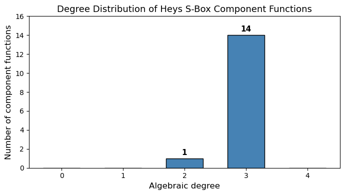
Degree of each component function (lambda=1..15):
  lambda= 1 (0b0001): degree 3
  lambda= 2 (0b0010): degree 3
  lambda= 3 (0b0011): degree 3
  lambda= 4 (0b0100): degree 3
  lambda= 5 (0b0101): degree 2
  lambda= 6 (0b0110): degree 3
  lambda= 7 (0b0111): degree 3
  lambda= 8 (0b1000): degree 3
  lambda= 9 (0b1001): degree 3
  lambda=10 (0b1010): degree 3
  lambda=11 (0b1011): degree 3
  lambda=12 (0b1100): degree 3
  lambda=13 (0b1101): degree 3
  lambda=14 (0b1110): degree 3
  lambda=15 (0b1111): degree 3

Observation

All 15 component functions of the Heys S-box have degree 3 – the maximum achievable for a 4-bit permutation S-box (degree 4 is impossible for a balanced function on 4 variables, since the monomial \(x_0 x_1 x_2 x_3\) evaluates to 1 on only one input). This uniform high degree is a sign of good algebraic resistance. (In general, some permutation S-boxes may have component functions with degrees ranging from 2 to 3.)

35.10 Algebraic Immunity#

Computing the algebraic immunity requires checking whether there exists a nonzero function \(g\) of degree \(\leq d\) such that \(f \cdot g = 0\) (i.e., \(g\) vanishes on the support of \(f\)) or \((1 \oplus f) \cdot g = 0\) (i.e., \(g\) vanishes on the support of \(1 \oplus f\)).

We solve this by constructing a matrix of all monomials up to degree \(d\) evaluated at the support points, and checking if this matrix has a nontrivial null-space over \(\text{GF}(2)\).

import numpy as np
from itertools import combinations

def _gf2_rank(matrix):
    """Compute the rank of a binary matrix over GF(2) via Gaussian elimination."""
    M = np.array(matrix, dtype=np.int64) % 2
    rows, cols = M.shape
    rank = 0
    for col in range(cols):
        # Find pivot
        pivot = None
        for row in range(rank, rows):
            if M[row, col] == 1:
                pivot = row
                break
        if pivot is None:
            continue
        # Swap
        M[[rank, pivot]] = M[[pivot, rank]]
        # Eliminate
        for row in range(rows):
            if row != rank and M[row, col] == 1:
                M[row] = (M[row] + M[rank]) % 2
        rank += 1
    return rank

def _monomials_up_to_degree(n, d):
    """Return all monomial indices u with Hamming weight <= d."""
    indices = []
    for u in range(1 << n):
        if hamming_weight(u) <= d:
            indices.append(u)
    return indices

def _evaluate_monomial(u, x, n):
    """Evaluate monomial u at point x (both integers encoding bit vectors)."""
    # Monomial u: product of x_i for i where u has bit i set
    # This equals 1 iff all bits of u are also set in x
    return 1 if (x & u) == u else 0

def _has_annihilator(support_points, n, d):
    """Check if there is a nonzero polynomial of degree <= d vanishing on all support points."""
    mono_indices = _monomials_up_to_degree(n, d)
    n_monos = len(mono_indices)
    n_pts = len(support_points)
    
    if n_pts == 0:
        return True  # the constant 1 annihilates the empty set
    
    # Build evaluation matrix: rows = support points, cols = monomials
    M = np.zeros((n_pts, n_monos), dtype=np.int64)
    for i, x in enumerate(support_points):
        for j, u in enumerate(mono_indices):
            M[i, j] = _evaluate_monomial(u, x, n)
    
    # A nonzero annihilator exists iff rank(M) < n_monos
    r = _gf2_rank(M)
    return r < n_monos

def algebraic_immunity(tt):
    """Compute the algebraic immunity of a Boolean function.
    
    Parameters
    ----------
    tt : array-like of int
        Truth table of length 2**n, entries in {0, 1}.
    
    Returns
    -------
    ai : int
        The algebraic immunity.
    """
    tt = np.asarray(tt, dtype=np.int64)
    N = len(tt)
    n = int(np.log2(N))
    
    # Support of f and 1+f
    supp_f = [x for x in range(N) if tt[x] == 1]
    supp_1f = [x for x in range(N) if tt[x] == 0]
    
    for d in range(0, n + 1):
        if _has_annihilator(supp_f, n, d) or _has_annihilator(supp_1f, n, d):
            return d
    return n  # should not reach here for a proper Boolean function

# Test on a simple function: f(x0,x1) = x0 AND x1
tt_and = [0, 0, 0, 1]
print(f"AI of x0*x1: {algebraic_immunity(tt_and)}")

# Test on XOR
tt_xor = [0, 1, 1, 0]
print(f"AI of x0+x1: {algebraic_immunity(tt_xor)}")

AI of x0*x1: 1
AI of x0+x1: 1

35.11 Algebraic Immunity of the Heys S-Box#

import numpy as np

SBOX = np.array([0xE, 0x4, 0xD, 0x1, 0x2, 0xF, 0xB, 0x8,
                 0x3, 0xA, 0x6, 0xC, 0x5, 0x9, 0x0, 0x7], dtype=np.int64)
n_bits = 4
N = 1 << n_bits

print("Algebraic immunity of Heys S-box coordinate functions:")
print("=" * 55)
for bit in range(n_bits):
    tt = (SBOX >> bit) & 1
    ai = algebraic_immunity(tt)
    print(f"  y{bit}: AI = {ai}")

print("\nAlgebraic immunity of all 15 component functions:")
print("-" * 55)
ai_values = []
for lam in range(1, N):
    tt = np.zeros(N, dtype=np.int64)
    for j in range(n_bits):
        if (lam >> j) & 1:
            tt ^= (SBOX >> j) & 1
    ai = algebraic_immunity(tt)
    ai_values.append(ai)
    print(f"  lambda={int(lam):2d} (0b{lam:04b}): AI = {ai}")

print(f"\nMinimum AI: {min(ai_values)}")
print(f"Maximum AI: {max(ai_values)}")
print(f"Maximum possible for n=4: {(n_bits + 1) // 2}")

Algebraic immunity of Heys S-box coordinate functions:
=======================================================
  y0: AI = 2
  y1: AI = 2
  y2: AI = 2
  y3: AI = 2

Algebraic immunity of all 15 component functions:
-------------------------------------------------------
  lambda= 1 (0b0001): AI = 2
  lambda= 2 (0b0010): AI = 2
  lambda= 3 (0b0011): AI = 2
  lambda= 4 (0b0100): AI = 2
  lambda= 5 (0b0101): AI = 2
  lambda= 6 (0b0110): AI = 2
  lambda= 7 (0b0111): AI = 2
  lambda= 8 (0b1000): AI = 2
  lambda= 9 (0b1001): AI = 2
  lambda=10 (0b1010): AI = 2
  lambda=11 (0b1011): AI = 2
  lambda=12 (0b1100): AI = 2
  lambda=13 (0b1101): AI = 2
  lambda=14 (0b1110): AI = 2
  lambda=15 (0b1111): AI = 2

Minimum AI: 2
Maximum AI: 2
Maximum possible for n=4: 2

Interpretation

For a balanced Boolean function on \(n = 4\) variables, the maximum possible algebraic immunity is \(\lceil 4/2 \rceil = 2\). If any component function has \(\text{AI} = 1\), it means there exists a linear annihilator – a devastating weakness for algebraic attacks. An \(\text{AI}\) of 2 is optimal for \(n = 4\).

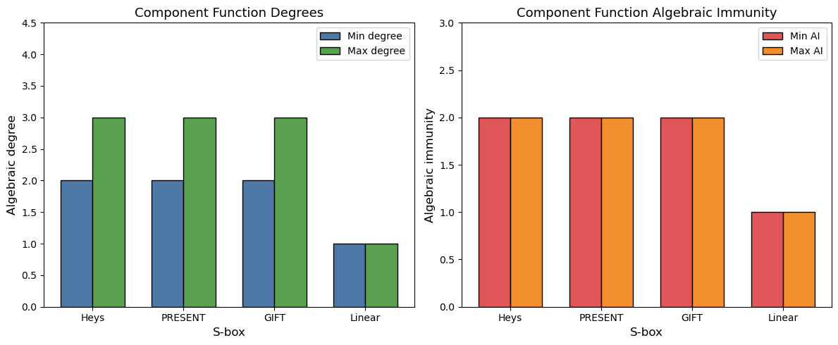
35.12 Comparing S-Boxes: Algebraic Properties#

Let us compare the Heys S-box with several other 4-bit S-boxes to see how algebraic properties vary.

Show code cell source Hide code cell source

import numpy as np
import matplotlib.pyplot as plt

# Several 4-bit S-boxes for comparison
sboxes = {
    "Heys":     [0xE, 0x4, 0xD, 0x1, 0x2, 0xF, 0xB, 0x8,
                 0x3, 0xA, 0x6, 0xC, 0x5, 0x9, 0x0, 0x7],
    "PRESENT":  [0xC, 0x5, 0x6, 0xB, 0x9, 0x0, 0xA, 0xD,
                 0x3, 0xE, 0xF, 0x8, 0x4, 0x7, 0x1, 0x2],
    "GIFT":     [0x1, 0xA, 0x4, 0xC, 0x6, 0xF, 0x3, 0x9,
                 0x2, 0xD, 0xB, 0x7, 0x5, 0x0, 0x8, 0xE],
    "Linear":   list(range(16)),  # identity (totally insecure)
}

n_bits = 4
N = 16
results = {}

for name, sbox in sboxes.items():
    sbox_arr = np.array(sbox, dtype=np.int64)
    comp_degrees = []
    comp_ais = []
    for lam in range(1, N):
        tt = np.zeros(N, dtype=np.int64)
        for j in range(n_bits):
            if (lam >> j) & 1:
                tt ^= (sbox_arr >> j) & 1
        anf = anf_from_truth_table(tt)
        comp_degrees.append(algebraic_degree(anf))
        comp_ais.append(algebraic_immunity(tt))
    results[name] = {
        "min_deg": min(comp_degrees),
        "max_deg": max(comp_degrees),
        "min_ai": min(comp_ais),
        "max_ai": max(comp_ais),
        "degrees": comp_degrees,
        "ais": comp_ais,
    }

# Print comparison table
print(f"{'S-box':<12} {'Min Deg':>8} {'Max Deg':>8} {'Min AI':>8} {'Max AI':>8}")
print("=" * 48)
for name, r in results.items():
    print(f"{name:<12} {r['min_deg']:>8} {r['max_deg']:>8} {r['min_ai']:>8} {r['max_ai']:>8}")

# Bar chart comparison
fig, (ax1, ax2) = plt.subplots(1, 2, figsize=(12, 5))

names = list(results.keys())
x = np.arange(len(names))
width = 0.35

min_degs = [results[n]["min_deg"] for n in names]
max_degs = [results[n]["max_deg"] for n in names]
min_ais = [results[n]["min_ai"] for n in names]
max_ais = [results[n]["max_ai"] for n in names]

ax1.bar(x - width/2, min_degs, width, label="Min degree", color="#4e79a7", edgecolor="black")
ax1.bar(x + width/2, max_degs, width, label="Max degree", color="#59a14f", edgecolor="black")
ax1.set_xlabel("S-box", fontsize=12)
ax1.set_ylabel("Algebraic degree", fontsize=12)
ax1.set_title("Component Function Degrees", fontsize=13)
ax1.set_xticks(x)
ax1.set_xticklabels(names)
ax1.legend()
ax1.set_ylim(0, n_bits + 0.5)

ax2.bar(x - width/2, min_ais, width, label="Min AI", color="#e15759", edgecolor="black")
ax2.bar(x + width/2, max_ais, width, label="Max AI", color="#f28e2b", edgecolor="black")
ax2.set_xlabel("S-box", fontsize=12)
ax2.set_ylabel("Algebraic immunity", fontsize=12)
ax2.set_title("Component Function Algebraic Immunity", fontsize=13)
ax2.set_xticks(x)
ax2.set_xticklabels(names)
ax2.legend()
ax2.set_ylim(0, 3)

plt.tight_layout()
plt.savefig("ch35_sbox_comparison.png", dpi=150, bbox_inches="tight")
plt.show()

S-box         Min Deg  Max Deg   Min AI   Max AI
================================================
Heys                2        3        2        2
PRESENT             2        3        2        2
GIFT                2        3        2        2
Linear              1        1        1        1

../_images/f6b517cedcb47c842e68f9d9e490f86ffb3fcb7391cdfd03aeaf7d23541b86fc.png

35.13 The ANF of the AES S-Box (Conceptual)#

The AES S-box operates on 8-bit inputs, so it has \(2^8 = 256\) entries and each component function is a Boolean function on 8 variables. The AES S-box is defined as inversion in \(\text{GF}(2^8)\) followed by an affine transformation.

AES S-Box Properties

Algebraic degree: 7 (the maximum for a balanced 8-bit function).
Algebraic immunity: 3 (below the optimum of 4).
The inverse map \(x \mapsto x^{-1}\) in \(\text{GF}(2^8)\) can be written as \(x^{254}\) (since \(x^{255} = 1\) for all \(x \neq 0\)).
The ANF of each coordinate function has 255 terms out of a possible 256 – it is almost maximally complex.
Each S-box application produces 39 quadratic equations in 16 variables (Courtois and Pieprzyk, 2002).

Despite the high degree and term count, the specific algebraic structure of inversion in \(\text{GF}(2^8)\) gives rise to overdefined systems of quadratic equations when the S-box is modeled implicitly. This is the foundation of the XSL attack.

We can compute the degree of one coordinate of the AES S-box with our tools. Below we construct the 8-bit S-box table from the standard AES specification.

import numpy as np

# AES S-box (standard FIPS 197 table)
AES_SBOX = np.array([
    0x63, 0x7c, 0x77, 0x7b, 0xf2, 0x6b, 0x6f, 0xc5,
    0x30, 0x01, 0x67, 0x2b, 0xfe, 0xd7, 0xab, 0x76,
    0xca, 0x82, 0xc9, 0x7d, 0xfa, 0x59, 0x47, 0xf0,
    0xad, 0xd4, 0xa2, 0xaf, 0x9c, 0xa4, 0x72, 0xc0,
    0xb7, 0xfd, 0x93, 0x26, 0x36, 0x3f, 0xf7, 0xcc,
    0x34, 0xa5, 0xe5, 0xf1, 0x71, 0xd8, 0x31, 0x15,
    0x04, 0xc7, 0x23, 0xc3, 0x18, 0x96, 0x05, 0x9a,
    0x07, 0x12, 0x80, 0xe2, 0xeb, 0x27, 0xb2, 0x75,
    0x09, 0x83, 0x2c, 0x1a, 0x1b, 0x6e, 0x5a, 0xa0,
    0x52, 0x3b, 0xd6, 0xb3, 0x29, 0xe3, 0x2f, 0x84,
    0x53, 0xd1, 0x00, 0xed, 0x20, 0xfc, 0xb1, 0x5b,
    0x6a, 0xcb, 0xbe, 0x39, 0x4a, 0x4c, 0x58, 0xcf,
    0xd0, 0xef, 0xaa, 0xfb, 0x43, 0x4d, 0x33, 0x85,
    0x45, 0xf9, 0x02, 0x7f, 0x50, 0x3c, 0x9f, 0xa8,
    0x51, 0xa3, 0x40, 0x8f, 0x92, 0x9d, 0x38, 0xf5,
    0xbc, 0xb6, 0xda, 0x21, 0x10, 0xff, 0xf3, 0xd2,
    0xcd, 0x0c, 0x13, 0xec, 0x5f, 0x97, 0x44, 0x17,
    0xc4, 0xa7, 0x7e, 0x3d, 0x64, 0x5d, 0x19, 0x73,
    0x60, 0x81, 0x4f, 0xdc, 0x22, 0x2a, 0x90, 0x88,
    0x46, 0xee, 0xb8, 0x14, 0xde, 0x5e, 0x0b, 0xdb,
    0xe0, 0x32, 0x3a, 0x0a, 0x49, 0x06, 0x24, 0x5c,
    0xc2, 0xd3, 0xac, 0x62, 0x91, 0x95, 0xe4, 0x79,
    0xe7, 0xc8, 0x37, 0x6d, 0x8d, 0xd5, 0x4e, 0xa9,
    0x6c, 0x56, 0xf4, 0xea, 0x65, 0x7a, 0xae, 0x08,
    0xba, 0x78, 0x25, 0x2e, 0x1c, 0xa6, 0xb4, 0xc6,
    0xe8, 0xdd, 0x74, 0x1f, 0x4b, 0xbd, 0x8b, 0x8a,
    0x70, 0x3e, 0xb5, 0x66, 0x48, 0x03, 0xf6, 0x0e,
    0x61, 0x35, 0x57, 0xb9, 0x86, 0xc1, 0x1d, 0x9e,
    0xe1, 0xf8, 0x98, 0x11, 0x69, 0xd9, 0x8e, 0x94,
    0x9b, 0x1e, 0x87, 0xe9, 0xce, 0x55, 0x28, 0xdf,
    0x8c, 0xa1, 0x89, 0x0d, 0xbf, 0xe6, 0x42, 0x68,
    0x41, 0x99, 0x2d, 0x0f, 0xb0, 0x54, 0xbb, 0x16,
], dtype=np.int64)

# Compute degree of each coordinate function of the AES S-box
print("Algebraic degree of AES S-box coordinate functions:")
print("=" * 50)
for bit in range(8):
    tt = (AES_SBOX >> bit) & 1
    anf = anf_from_truth_table(tt)
    deg = algebraic_degree(anf)
    n_terms = np.count_nonzero(anf)
    print(f"  Bit {bit}: degree = {deg}, active terms = {n_terms}/256")

Algebraic degree of AES S-box coordinate functions:
==================================================
  Bit 0: degree = 7, active terms = 132/256
  Bit 1: degree = 7, active terms = 133/256
  Bit 2: degree = 7, active terms = 145/256
  Bit 3: degree = 7, active terms = 136/256
  Bit 4: degree = 7, active terms = 131/256
  Bit 5: degree = 7, active terms = 114/256
  Bit 6: degree = 7, active terms = 112/256
  Bit 7: degree = 7, active terms = 110/256

35.14 Visualizing ANF Term Density#

We can visualize which monomials appear in each coordinate function by plotting the ANF coefficient vectors as a heatmap. Dark cells indicate active monomials (\(a_u = 1\)).

../_images/7f68cd7c341ccb889c0279a38ec2eceab7d2c02351c6069f5b6c721a34f5cb07.png

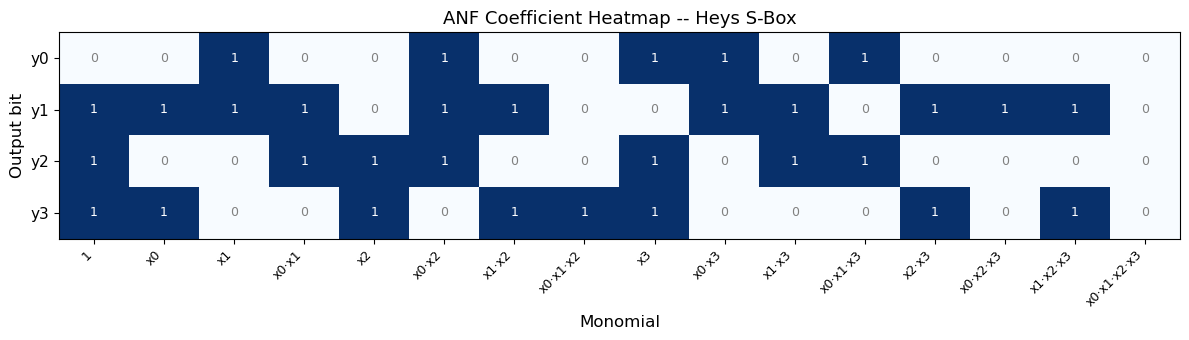
Total active terms: 31/64 (48.4%)

35.15 Verifying the Algebraic Model: S-Box Round-Trip#

As a sanity check, we verify that evaluating the ANF polynomials reproduces the original S-box lookup table for every input.

import numpy as np

SBOX = np.array([0xE, 0x4, 0xD, 0x1, 0x2, 0xF, 0xB, 0x8,
                 0x3, 0xA, 0x6, 0xC, 0x5, 0x9, 0x0, 0x7], dtype=np.int64)
n_bits = 4
N = 16

# Compute ANFs
anfs = []
for bit in range(n_bits):
    tt = (SBOX >> bit) & 1
    anfs.append(anf_from_truth_table(tt))

# Evaluate ANFs at every input and reconstruct S-box output
all_correct = True
print(f"{'Input':>6} {'Expected':>9} {'Computed':>9} {'Match':>6}")
print("-" * 35)
for x in range(N):
    computed_bits = []
    for bit in range(n_bits):
        # Evaluate ANF at point x
        val = 0
        for u in range(N):
            if anfs[bit][u] == 1:
                # Monomial u evaluates to 1 iff (x & u) == u
                if (x & u) == u:
                    val ^= 1
        computed_bits.append(val)
    computed = sum(b << i for i, b in enumerate(computed_bits))
    expected = SBOX[x]
    match = computed == expected
    if not match:
        all_correct = False
    print(f"{x:>6} (0x{x:X})  0x{expected:X}       0x{computed:X}     {'OK' if match else 'FAIL'}")

print(f"\nAll entries match: {all_correct}")

 Input  Expected  Computed  Match
-----------------------------------
(0x0)  0xE       0xE     OK
(0x1)  0x4       0x4     OK
(0x2)  0xD       0xD     OK
(0x3)  0x1       0x1     OK
(0x4)  0x2       0x2     OK
(0x5)  0xF       0xF     OK
(0x6)  0xB       0xB     OK
(0x7)  0x8       0x8     OK
(0x8)  0x3       0x3     OK
(0x9)  0xA       0xA     OK
(0xA)  0x6       0x6     OK
(0xB)  0xC       0xC     OK
(0xC)  0x5       0x5     OK
(0xD)  0x9       0x9     OK
(0xE)  0x0       0x0     OK
(0xF)  0x7       0x7     OK

All entries match: True

35.16 Degree Growth Through S-Box Composition#

When S-boxes are composed (as in multiple rounds of a cipher), the algebraic degree of the resulting function grows. For a single S-box of degree \(d\) applied \(r\) times, the degree can grow up to \(d^r\) (bounded by \(2^n - 1\)). Let us measure this experimentally.

../_images/31a40d92ce6cd279b7d244432517e2c697d015d5dbbe74ea5fde604142eba427.png

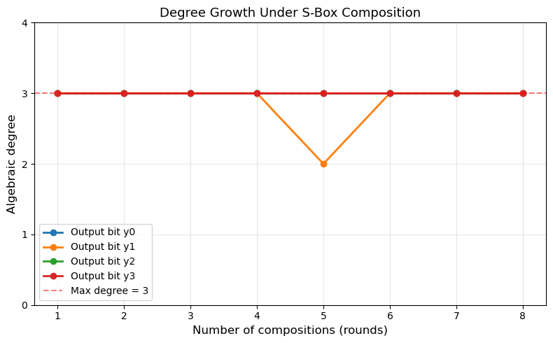
 Round    y0   y1   y2   y3   max
-----------------------------------
   3    3    3    3     3
   3    3    3    3     3
   3    3    3    3     3
   3    3    3    3     3
   3    2    3    3     3
   3    3    3    3     3
   3    3    3    3     3
   3    3    3    3     3

Degree Saturation

The degree quickly saturates at 3 (the maximum for a balanced 4-bit permutation). In a real cipher, key addition between rounds prevents simple composition, but the degree growth still tells us that after a few rounds, the algebraic expressions become very complex – this is the cipher’s defense against algebraic attacks.

35.17 Monomial Count Growth#

Another indicator of algebraic complexity is how the number of active monomials in the ANF grows with the number of S-box compositions.

../_images/332814bf358ad0c5de2651fedd20685bb7080f89b058f05dce71b40691cb10c1.png

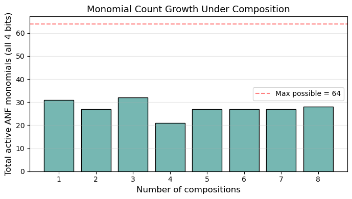
  Round 1: 31/64 terms (48.4%)
  Round 2: 27/64 terms (42.2%)
  Round 3: 32/64 terms (50.0%)
  Round 4: 21/64 terms (32.8%)
  Round 5: 27/64 terms (42.2%)
  Round 6: 27/64 terms (42.2%)
  Round 7: 27/64 terms (42.2%)
  Round 8: 28/64 terms (43.8%)

35.18 Exercises#

Exercise 35.1 (ANF by hand)

Compute the ANF of the Boolean function \(f : \text{GF}(2)^3 \to \text{GF}(2)\) with truth table \((0, 1, 1, 0, 1, 0, 0, 1)\). What is its algebraic degree?

Hint

Apply the Mobius transform: for each index \(u\), compute \(a_u = \bigoplus_{v \preceq u} f(v)\), where \(v \preceq u\) means that every bit of \(v\) is \(\leq\) the corresponding bit of \(u\). The degree equals the maximum Hamming weight among indices with \(a_u = 1\). This particular truth table is the 3-variable XOR function \(x_0 \oplus x_1 \oplus x_2\).

Exercise 35.2 (Affine functions)

Prove that a Boolean function has algebraic degree \(\leq 1\) if and only if it is affine (i.e., \(f(x) = a_0 \oplus a_1 x_1 \oplus \cdots \oplus a_n x_n\)). Why are affine S-boxes catastrophically insecure?

Hint

Degree \(\leq 1\) means the ANF has no monomials of degree 2 or higher, so \(f\) is a linear combination of variables plus a constant – this is exactly the definition of affine. An affine S-box means the entire cipher is a system of linear equations over \(\text{GF}(2)\), solvable by Gaussian elimination with a single known plaintext–ciphertext pair.

Exercise 35.3 (Annihilators)

Find a nonzero Boolean function \(g\) on 4 variables such that \(f \cdot g = 0\), where \(f\) is the output bit \(y_0\) of the Heys S-box. What is the degree of \(g\)?

Hint

The support of \(y_0\) (where it equals 1) has 8 elements. You need a function \(g\) that equals 0 on all these 8 points but is nonzero elsewhere. Build the evaluation matrix of all monomials up to some degree \(d\) at the support points, and find the null space over \(\text{GF}(2)\). Start with \(d = 2\).

Exercise 35.4 (Random S-box algebraic properties)

Generate 100 random 4-bit permutation S-boxes and compute the minimum component-function degree and minimum algebraic immunity for each. Plot histograms. How does the Heys S-box compare to a “typical” random permutation?

Hint

Use np.random.permutation(16) to generate random permutation S-boxes. For each, compute degrees and algebraic immunities of all 15 component functions. Most random 4-bit permutations will have all component functions at degree 3, but a small fraction may have degree-2 component functions. Compare the distribution of minimum AI values.

Exercise 35.5 (Scaling analysis)

For the 3-round SPN with \(n\)-bit S-boxes and a block size of \(4n\) bits (four S-boxes per round), derive formulas for the number of variables and equations as a function of \(n\). At what value of \(n\) does the system become underdefined (more variables than equations)?

Hint

Use the counting approach from Section 35.8. The key observation is that the number of field equations grows linearly with the number of variables, while the ANF equations grow with the number of S-box applications times \(n\). Since each S-box application also introduces \(2n\) new variables but only \(n\) ANF equations, larger S-boxes tend to produce underdefined systems unless additional equations (e.g., from multiple plaintext–ciphertext pairs) are added.

35.19 Summary#

In this chapter we developed a toolkit for the algebraic analysis of S-boxes and applied it to the Heys 4-bit S-box and the AES S-box.

Key takeaways:

Every Boolean function has a unique ANF, computable via the Mobius transform in \(O(n \cdot 2^n)\) time.
The algebraic degree measures the complexity of the polynomial representation. Higher degree makes algebraic attacks harder.
The algebraic immunity measures resistance to annihilator-based attacks. The optimum for \(n\) variables is \(\lceil n/2 \rceil\).
An S-box with \(n\)-bit inputs and \(m\)-bit outputs generates \(m\) polynomial equations in \(n + m\) variables. Across multiple rounds of a cipher, these equations accumulate into a large (often overdefined) system.
The Heys S-box has degree 3 and algebraic immunity 2 for all component functions – both optimal for a 4-bit permutation.
The AES S-box has degree 7 (optimal for 8-bit) but algebraic immunity 3 (below the optimum of 4), which is a known structural property of the inversion map in \(\text{GF}(2^8)\).

References:

G. V. Bard, Algebraic Cryptanalysis, Springer, 2009.
N. T. Courtois and J. Pieprzyk, “Cryptanalysis of Block Ciphers with Overdefined Systems of Equations,” ASIACRYPT 2002.
C. Carlet, Boolean Functions for Cryptography and Coding Theory, Cambridge University Press, 2021.
M. S. E. Mohamed, W. S. A. E. Mohamed, J. Ding, and J. Buchmann, “MXL2: Solving Polynomial Equations over GF(2) Using an Improved Mutant Strategy,” PQCrypto 2008.

Chapter 35: Algebraic Modeling of S-Boxes

Contents

Chapter 35: Algebraic Modeling of S-Boxes#

35.1 Introduction#

35.2 Definitions#

35.3 The Mobius Transform: From Truth Table to ANF#

35.4 Algebraic Degree Computation#

35.5 Displaying the ANF as a Polynomial String#

35.6 The Heys S-Box: ANF of Each Output Bit#

35.7 Generating Polynomial Equations for an S-Box#

35.8 Equation Counts for a Multi-Round SPN#

35.9 Degree Distribution of S-Box Component Functions#

35.10 Algebraic Immunity#

35.11 Algebraic Immunity of the Heys S-Box#

35.12 Comparing S-Boxes: Algebraic Properties#

35.13 The ANF of the AES S-Box (Conceptual)#

35.14 Visualizing ANF Term Density#

35.15 Verifying the Algebraic Model: S-Box Round-Trip#

35.16 Degree Growth Through S-Box Composition#

35.17 Monomial Count Growth#

35.18 Exercises#

35.19 Summary#