
Chapter 35: Algebraic Analysis of S-Boxes (SageMath)#
Python Version Available
This notebook contains the SageMath implementation using
PolynomialRing, GF(2), ideal(), .groebner_basis(), and
AffineSpace. A pure Python/NumPy version is available in
Chapter 35: Algebraic Analysis of S-Boxes.
35.1 Introduction#
Every S-box, no matter how complicated, is ultimately a mapping between finite sets of binary vectors. Because those vectors live in \(\text{GF}(2)^n\), each output bit of the S-box can be written as a multivariate polynomial over \(\text{GF}(2)\) in the input bits. This representation is the Algebraic Normal Form (ANF).
Key Idea
Every S-box can be expressed as a system of polynomial equations over \(\text{GF}(2)\). This enables algebraic attacks: if we can collect enough plaintext–ciphertext pairs, we obtain a system of multivariate quadratic (or low-degree) equations whose solution reveals the key.
The feasibility of algebraic attacks depends on two quantities:
The algebraic degree of the S-box – lower degree means easier equations.
The algebraic immunity – the minimum degree of a nonzero function \(g\) such that \(f \cdot g = 0\) or \((1 \oplus f) \cdot g = 0\).
In this chapter we use SageMath to perform algebraic cryptanalysis of S-boxes. We model a 3-bit S-box as a system of polynomial equations over \(\text{GF}(2)\), compute Groebner bases, build a full substitution-permutation network (SPN), and use ideal-theoretic tools (elimination ideals, irreducible components) to reveal structural weaknesses in the cipher.
References:
G. V. Bard, Algebraic Cryptanalysis, Springer, 2009.
N. T. Courtois and G. V. Bard, “Algebraic Cryptanalysis of the Data Encryption Standard,” IMA 2007.
N. T. Courtois and J. Pieprzyk, “Cryptanalysis of Block Ciphers with Overdefined Systems of Equations,” ASIACRYPT 2002.
35.2 Definitions#
We work with Boolean functions \(f : \text{GF}(2)^n \to \text{GF}(2)\) and vectorial Boolean functions (S-boxes) \(S : \text{GF}(2)^n \to \text{GF}(2)^m\).
Definition 35.1 – Algebraic Normal Form (ANF)
Every Boolean function \(f : \text{GF}(2)^n \to \text{GF}(2)\) can be uniquely written as
where \(u = (u_1, \ldots, u_n)\) ranges over all \(2^n\) binary vectors. The coefficients \(a_u\) are computed from the truth table via the Mobius transform (inclusion–exclusion over \(\text{GF}(2)\)).
Definition 35.2 – Algebraic Degree
The algebraic degree of \(f\) is the maximum Hamming weight \(\text{wt}(u)\) over all \(u\) with \(a_u \neq 0\):
For an S-box \(S = (f_1, \ldots, f_m)\), the algebraic degree is \(\deg(S) = \max_i \deg(f_i)\).
Definition 35.3 – Algebraic Immunity
The algebraic immunity \(\text{AI}(f)\) of a Boolean function \(f\) is the minimum degree \(d\) such that there exists a nonzero function \(g\) of degree \(d\) satisfying \(f \cdot g = 0\) or \((1 \oplus f) \cdot g = 0\) (where multiplication and addition are in \(\text{GF}(2)\), evaluated pointwise over all inputs).
A high algebraic immunity makes algebraic attacks harder. The maximum possible value for \(n\)-variable functions is \(\lceil n/2 \rceil\).
Definition 35.4 – Groebner Basis
A Groebner basis of a polynomial ideal \(I\) is a generating set \(G = \{g_1, \ldots, g_s\}\) such that the leading term ideal \(\langle \text{LT}(g_1), \ldots, \text{LT}(g_s) \rangle = \langle \text{LT}(I) \rangle\). In the context of \(\text{GF}(2)\), computing a Groebner basis effectively solves the system of polynomial equations, yielding the variety of the ideal.
35.3 Modeling a 3-Bit S-Box#
We begin by modeling a 3-bit S-box as a permutation on \(\{0, 1, \ldots, 7\}\).
The helper functions C1 and Ci convert between integer and
binary-vector representations using SageMath’s ZZ ring.
#modeling an SBox 3bits - 3 bits
perm=[1,3,2,0,5,7,4,6]
def C1(a):
    return ZZ(a).digits(base=2,padto=3)

def Ci(b):
    return int(''.join(map(str,b[::-1])),base=2)
def SBox(b3):
    n=perm[Ci(b3)]
    return C1(n)
Let us verify the S-box on a few inputs:
SBox([0,0,0])
[1, 0, 0]
SBox([0,0,1])
[1, 0, 1]
35.4 Algebraic Model of the S-Box#
Each output bit of the S-box can be written as a polynomial in the input variables over \(\text{GF}(2)\). For 3 input bits, the most general degree-2 polynomial has 7 coefficients: a constant \(a_0\), three linear terms \(a_1 x_1, a_2 x_2, a_3 x_3\), and three quadratic terms \(a_{12} x_1 x_2, a_{13} x_1 x_3, a_{23} x_2 x_3\).
#algebraic model of the Sbox output using polynomials in the input variables
def AlgSBox(A,X):
    a0,a1,a2,a3,a12,a13,a23=A
    x1,x2,x3=X
    return a0 + a1*x1 + a2*x2 + a3*x3+a12*x1*x2 + a13*x1*x3 + a23*x2*x3
R.<a0,a1,a2,a3,a12,a13,a23>=PolynomialRing(GF(2),7)
A=[a0,a1,a2,a3,a12,a13,a23]
35.5 Solving for the ANF Coefficients via Groebner Bases#
For each output bit, we set up the system of equations \(\text{AlgSBox}(A, C1(n)) - \text{SBox}(C1(n))[i] = 0\) for all inputs \(n \in \{0, \ldots, 6\}\). The Groebner basis of the resulting ideal gives us the unique polynomial coefficients.
Interpretation of ANF Indices
The index \(u\) in the ANF vector encodes a monomial via its binary representation. For \(n = 3\) variables \((x_1, x_2, x_3)\):
Index \(u\) |
Binary |
Monomial |
|---|---|---|
0 |
000 |
1 (constant) |
1 |
001 |
\(x_1\) |
2 |
010 |
\(x_2\) |
3 |
011 |
\(x_1 x_2\) |
4 |
100 |
\(x_3\) |
5 |
101 |
\(x_1 x_3\) |
6 |
110 |
\(x_2 x_3\) |
7 |
111 |
\(x_1 x_2 x_3\) |
eqs=lambda n,i: AlgSBox(A,C1(n))-SBox(C1(n))[i]
Output bit 0#
I0=R.ideal([eqs(n,0) for n in range(0,7)])
I0.groebner_basis()
[a0 + 1, a1, a2 + 1, a3, a12, a13, a23]
RX.<x1,x2,x3>=PolynomialRing(GF(2),3)
Spol0=1+x2
Interpretation
The Groebner basis tells us that the zeroth output bit is \(y_0 = 1 + x_2\). The coefficient variables are uniquely determined by the ideal, so the ANF is exact.
Output bit 1#
I1=R.ideal([eqs(n,1) for n in range(0,7)])
I1.groebner_basis()
[a0, a1 + 1, a2 + 1, a3, a12, a13, a23 + 1]
Spol1=x1+x2+x2*x3
Output bit 2#
I2=R.ideal([eqs(n,2) for n in range(0,7)])
I2.groebner_basis()
[a0, a1, a2, a3 + 1, a12, a13, a23]
Spol2=x3
Summary of ANF Polynomials
The S-box is fully described by three polynomials over \(\text{GF}(2)\):
The algebraic degree of this S-box is 2 (from the \(x_2 x_3\) term in \(y_1\)). Note that \(y_0\) and \(y_2\) are affine (degree 1), which already hints at a structural weakness.
35.6 Verifying the Algebraic S-Box Model#
We verify that our polynomial model reproduces the S-box lookup table for every input.
def SBoxModel(v):
    v1,v2,v3=v
    return [Spol0.subs({x1:v1,x2:v2,x3:v3}),Spol1.subs({x1:v1,x2:v2,x3:v3}),Spol2.subs({x1:v1,x2:v2,x3:v3})]
inputs=[C1(n) for n in range(8)]
for v in inputs:
    print(v)
    print(SBoxModel(v) == SBox(v))
[0, 0, 0]
True
[1, 0, 0]
True
[0, 1, 0]
True
[1, 1, 0]
True
[0, 0, 1]
True
[1, 0, 1]
True
[0, 1, 1]
True
[1, 1, 1]
True
So we have a working algebraic model of our S-box, which uses three polynomials in three variables over a field \(\mathbb{F}_{2}\).
Observation
The SageMath approach is fundamentally different from the Python version’s Mobius transform: instead of operating on truth-table vectors with XOR butterflies, we set up a symbolic polynomial system and use Groebner bases to solve for the ANF coefficients. Both produce the same result, but the SageMath approach generalizes naturally to more complex algebraic analyses.
35.7 Building the Substitution-Permutation Network (SPN)#
We now construct an SPN that in three rounds (plus a final key addition) weaves a 6-bit plaintext with a 6-bit key. The network consists of:
Key mixing (XOR with a round key),
Substitution (applying the 3-bit S-box to each half),
Permutation (rewiring the bits).
We trace the algebraic dependence of the output on the input and key.
Permutation layer#
#Permutation P
Plist=[1,0,2,4,3,5]

G = SymmetricGroup(range(0,6))
Pperm=PermutationGroupElement(Plist,G)

Pinvlist=[(Pperm**(-1))(i) for i in range(0,6)]

def P(block6):
    return [block6[x] for x in Plist]
def Pinv(block6):
    return [block6[x] for x in Pinvlist]
Key mixing (XOR over GF(2))#
#XORing lists
def ListXOR(li1,li2):
    return [li1[i]+li2[i] for i in range(0,len(li1))]
Note on GF(2) Arithmetic
Over \(\text{GF}(2)\), addition is the same as XOR. Since our
polynomial ring is already defined over \(\text{GF}(2)\), the +
operator in SageMath performs XOR automatically.
Key schedule and S-box layer#
#Key schedule
def KeySchedule(key6):
    k0,k1,k2,k3,k4,k5=key6
    return [[k0,k1,k2,k3,k4,k5],[k3,k4,k5,k0,k1,k2],[k0,k2,k4,k1,k3,k5],[k1,k1,k0,k0,k2,k2]]

def RoundKey(expkey,r):
    return expkey[r]

def S(block6):
    Sout=[]
    for i in range(0,2):
        Sout+=SBoxModel(block6[3*i:3*(i+1)])
    return Sout
Full SPN encryption#
def SPNEncryption(plaintext6,key6):
    expkey=KeySchedule(key6)
    state=plaintext6

    #round 1
    state=ListXOR(state,RoundKey(expkey,0))
    state=S(state)
    state=P(state)

    #round 2
    state=ListXOR(state,RoundKey(expkey,1))
    state=S(state)
    state=P(state)

    #round 3

    state=ListXOR(state,RoundKey(expkey,2))
    state=S(state)

    #final XOR
    state=ListXOR(state,RoundKey(expkey,3))

    return state
35.8 Generating Polynomial Equations for the SPN#
We now set up the full algebraic system. The coordinate ring has 18 variables: 6 plaintext bits, 6 key bits, and 6 ciphertext bits. All variables satisfy the Boolean field equations \(v_i^2 - v_i = 0\).
Key Idea
By working in the quotient ring \(R / \langle v_i^2 - v_i \rangle\), we enforce that every variable is Boolean. This is essential for the Groebner basis computation to produce finite solutions.
#coordinate ring
R.<p0,p1,p2,p3,p4,p5,k0,k1,k2,k3,k4,k5,c0,c1,c2,c3,c4,c5>=PolynomialRing(GF(2),18)

plaintext6=[p0,p1,p2,p3,p4,p5]
key6=[k0,k1,k2,k3,k4,k5]
cipher6=[c0,c1,c2,c3,c4,c5]

#Boolean relations
v=plaintext6+key6+cipher6
boolI=R.ideal([v[i]^2-v[i] for i in range(18)])
Q=R.quotient_ring(boolI)
Symbolic encryption model#
We pass symbolic variables through the encryption function. The output is a list of 6 polynomial expressions in the plaintext and key variables.
#encryption model
encryption6=SPNEncryption(plaintext6,key6)
pretty_print(encryption6)
Observation
Each ciphertext bit is now expressed as a multivariate polynomial in the plaintext and key bits over \(\text{GF}(2)\). These expressions grow in complexity with each round due to the nonlinear S-box substitutions.
35.9 Groebner Basis of the Cipher#
Relations
We form the ideal generated by the equations \(c_i - E_i(p, k) = 0\) for each ciphertext bit, lifted from the quotient ring (so that Boolean constraints are incorporated). The Groebner basis of this ideal captures all algebraic relations between plaintext, key, and ciphertext.
#detecting cipher-plaintext collisions
relI=R.ideal([Q(cipher6[i]-encryption6[i]).lift() for i in range(6)])
pretty_print(relI)
relI.groebner_basis()
[k0*k1 + k2^2 + k0*k4 + k1*k5 + k2*k5 + k4*k5 + k0*c0 + k5*c0 + k1*c2 + k4*c2 + c0*c2 + p0 + k2 + k3 + k4 + k5 + c0 + c1,
 k2*k3 + k1*k5 + k0*c5 + k1*c5 + c3*c5 + p3 + k3 + k5 + c3 + c4,
 p1 + k2 + k4 + c0 + 1,
 p2 + k0 + k2 + k4 + k5 + c2,
 p4 + k0 + k1 + k3 + k4 + c3 + 1,
 p5 + c5]
Irreducible components of the solution variety#
The irreducible components of the affine subscheme defined by our ideal show the distinct solution branches.
AffineSpace(R).subscheme(relI).irreducible_components()
[Closed subscheme of Affine Space of dimension 18 over Finite Field of size 2 defined by:
   p5 + c5,
   p4 + k0 + k1 + k3 + k4 + c3 + 1,
   p2 + k0 + k2 + k4 + k5 + c2,
   p1 + k2 + k4 + c0 + 1,
   k2*k3 + k1*k5 + k0*c5 + k1*c5 + c3*c5 + p3 + k3 + k5 + c3 + c4,
   k0*k1 + k2^2 + k0*k4 + k1*k5 + k2*k5 + k4*k5 + k0*c0 + k5*c0 + k1*c2 + k4*c2 + c0*c2 + p0 + k2 + k3 + k4 + k5 + c0 + c1]
35.10 Key-Independent Relations: Elimination Ideals#
The most powerful application of Groebner bases in cryptanalysis is variable elimination. By eliminating the key variables from the ideal, we obtain relations between plaintext and ciphertext that hold regardless of the key. These reveal structural flaws in the cipher design.
Key Idea
If the elimination ideal \(I \cap \mathbb{F}_2[p_0, \ldots, p_5, c_0, \ldots, c_5]\) is nontrivial, it means some plaintext-ciphertext relations are independent of the key – a catastrophic weakness.
#We check which output bits are independent of the key, hence directly decode some information about the input!
relI.elimination_ideal([k0,k1,k2,k3,k4,k5])
Ideal (p5 + c5) of Multivariate Polynomial Ring in p0, p1, p2, p3, p4, p5, k0, k1, k2, k3, k4, k5, c0, c1, c2, c3, c4, c5 over Finite Field of size 2
Critical Finding
The elimination ideal reveals that certain output bits are independent of the key! This means an attacker can directly decode some plaintext information from the ciphertext without knowing the key – a serious design flaw.
Partial key knowledge#
Even without eliminating all key variables, knowing just two key bits (\(k_4, k_5\)) suffices to reconstruct certain plaintext-ciphertext relations.
#the knowledge of just two bits of the key (k4,k5) would be enough to reconstruct certain relation of the input with output bits
rec=[Q(x).lift() for x in relI.elimination_ideal([k0,k1,k2,k3]).gens()]
rec
[p5 + c5,
 p1*p2*p4 + p1*p4*k4 + p2*p4*k4 + p1*p2*k5 + p1*p2*c0 + p2*p4*c0 + p1*k4*c0 + p2*k4*c0 + p4*k4*c0 + p1*k5*c0 + p1*p2*c2 + p1*k4*c2 + p2*k4*c2 + p2*c0*c2 + k4*c0*c2 + p1*p2*c3 + p1*k4*c3 + p2*k4*c3 + p2*c0*c3 + k4*c0*c3 + p1*k4*c5 + p2*k4*c5 + p2*k5*c5 + k4*k5*c5 + p1*c0*c5 + p2*c0*c5 + k4*c0*c5 + p1*c2*c5 + p2*c2*c5 + c0*c2*c5 + p1*c3*c5 + p2*c3*c5 + c0*c3*c5 + p0*p1 + p1*p3 + p2*p3 + p0*k4 + p1*k4 + p4*k4 + p0*k5 + p4*k5 + p0*c0 + p1*c0 + p2*c0 + p3*c0 + k5*c0 + p1*c1 + k4*c1 + k5*c1 + c0*c1 + k4*c2 + k5*c2 + p1*c3 + p2*c3 + k4*c3 + k5*c3 + c0*c3 + p1*c4 + p2*c4 + c0*c4 + p0*c5 + p1*c5 + p2*c5 + p4*c5 + k4*c5 + k5*c5 + c1*c5 + c2*c5 + c3*c5 + k4 + k5 + c0]
35.11 Concrete Attack: Known Ciphertext and Partial Key#
We now demonstrate a concrete attack scenario. Given a specific plaintext-key pair, we compute the ciphertext and then show how knowing just \((k_4, k_5)\) and the ciphertext allows us to drastically reduce the plaintext search space.
SPNEncryption([1,0,0,1,1,0],[0,1,1,0,1,0])
[1, 1, 0, 0, 1, 0]
R.ideal([Q(x).lift()
for x in R.ideal(relI.gens()+[k4-1,k5,c0-1,c1-1,c2,c3,c4-1,c5]).groebner_basis()]).groebner_basis()
[k0*k1 + p0 + k3 + 1,
 k2*k3 + p3 + k3 + 1,
 p1 + k2 + 1,
 p2 + k0 + k2 + 1,
 p4 + k0 + k1 + k3,
 p5,
 k4 + 1,
 k5,
 c0 + 1,
 c1 + 1,
 c2,
 c3,
 c4 + 1,
 c5]
AffineSpace(R).subscheme(R.ideal(rec +[k4-1,k5,c0-1,c1-1,c2,c3,c4-1,c5]).groebner_basis())
Closed subscheme of Affine Space of dimension 18 over Finite Field of size 2 defined by:
  p1*p2*p4 + p0*p1 + p1*p2 + p1*p3 + p2*p3 + p1*p4 + p1 + p2 + p3 + 1,
  p5,
  k4 + 1,
  k5,
  c0 + 1,
  c1 + 1,
  c2,
  c3,
  c4 + 1,
  c5
Counting surviving plaintexts#
We enumerate the rational points of the solution variety to see how many plaintext candidates survive the algebraic constraints.
A.<P0,P1,P2,P3,P4,P5>=AffineSpace(GF(2),6)
PS=A.subscheme([P1*P2*P4 + P0*P1 + P1*P2 + P1*P3 + P2*P3 + P1*P4 + P1 + P2 + P3 + 1,P5])
PS.rational_points()
[(0, 0, 0, 1, 0, 0),
 (0, 0, 0, 1, 1, 0),
 (0, 0, 1, 0, 0, 0),
 (0, 0, 1, 0, 1, 0),
 (0, 0, 1, 1, 0, 0),
 (0, 0, 1, 1, 1, 0),
 (0, 1, 0, 0, 0, 0),
 (0, 1, 0, 1, 0, 0),
 (0, 1, 1, 0, 0, 0),
 (0, 1, 1, 0, 1, 0),
 (1, 0, 0, 1, 0, 0),
 (1, 0, 0, 1, 1, 0),
 (1, 0, 1, 0, 0, 0),
 (1, 0, 1, 0, 1, 0),
 (1, 0, 1, 1, 0, 0),
 (1, 0, 1, 1, 1, 0),
 (1, 1, 0, 0, 1, 0),
 (1, 1, 0, 1, 1, 0),
 (1, 1, 1, 1, 0, 0),
 (1, 1, 1, 1, 1, 0)]
# the knowledge of a single ciphertext - (k4,k5) pair is enough to restrict the possibilities for the input by 70%
len(PS.rational_points())/2^6*1.0
0.312500000000000
Attack Impact
The knowledge of a single ciphertext and just 2 key bits (\(k_4, k_5\)) restricts the possible plaintexts to roughly 30% of the full space. This means about 70% of plaintext candidates are eliminated, a devastating reduction that would make brute-force search trivial.
35.12 Equation Counts for Multi-Round SPNs#
In a real attack, we compose S-box equations across multiple rounds. Each round introduces fresh intermediate variables, and the permutation layer just relabels wires.
For a 3-round SPN with block size 16 bits (four 4-bit S-boxes per round) and 4 round keys (each 16 bits, for \(n_{\text{rounds}} + 1 = 4\) key additions), let us count the equations and variables.
Overdefined Systems
When the number of equations exceeds the number of variables, the system is overdefined. This is precisely the situation that algebraic attacks exploit. Courtois and Pieprzyk (2002) showed that if one can generate sufficiently many low-degree equations, techniques like XL (eXtended Linearization) or Groebner bases can solve the system in polynomial time in the number of variables.
def count_spn_equations(n_rounds, block_bits, sbox_bits, n_sboxes_per_round):
    """Count equations and variables for an SPN algebraic model.

    Counts follow the standard modeling:
    - Each S-box application adds n_out ANF equations and
      n_in + n_out field equations.
    - Variables include: plaintext, ciphertext, round keys,
      and intermediate state bits.
    """
    n_sbox = sbox_bits

    # Variables
    n_plaintext = block_bits
    n_ciphertext = block_bits
    n_key_bits = (n_rounds + 1) * block_bits
    n_intermediate = n_rounds * 2 * block_bits

    total_vars = n_plaintext + n_ciphertext + n_key_bits + n_intermediate

    # Equations
    total_sbox_apps = n_rounds * n_sboxes_per_round
    anf_eqs = total_sbox_apps * n_sbox
    xor_eqs = (n_rounds + 1) * block_bits
    field_eqs = total_vars

    total_eqs = anf_eqs + xor_eqs + field_eqs

    return {
        "variables": total_vars,
        "plaintext_bits": n_plaintext,
        "ciphertext_bits": n_ciphertext,
        "key_bits": n_key_bits,
        "intermediate_bits": n_intermediate,
        "anf_equations": anf_eqs,
        "xor_equations": xor_eqs,
        "field_equations": field_eqs,
        "total_equations": total_eqs,
        "total_sbox_applications": total_sbox_apps,
    }

# 3-round SPN: 16-bit block, 4-bit S-boxes, 4 S-boxes per round
counts = count_spn_equations(
    n_rounds=3, block_bits=16, sbox_bits=4, n_sboxes_per_round=4
)

print("Algebraic model of a 3-round SPN (16-bit block, 4-bit S-boxes)")
print("=" * 65)
print(f"Plaintext bits:       {counts['plaintext_bits']}")
print(f"Ciphertext bits:      {counts['ciphertext_bits']}")
print(f"Key bits:             {counts['key_bits']}  ({counts['key_bits']//16} round keys x 16 bits)")
print(f"Intermediate bits:    {counts['intermediate_bits']}")
print(f"Total variables:      {counts['variables']}")
print()
print(f"S-box applications:   {counts['total_sbox_applications']}")
print(f"ANF equations:        {counts['anf_equations']}")
print(f"XOR equations:        {counts['xor_equations']}")
print(f"Field equations:      {counts['field_equations']}")
print(f"Total equations:      {counts['total_equations']}")
print()
print(f"Ratio (eqs/vars):     {float(counts['total_equations']/counts['variables']):.2f}")
Algebraic model of a 3-round SPN (16-bit block, 4-bit S-boxes)
=================================================================
Plaintext bits:       16
Ciphertext bits:      16
Key bits:             64  (4 round keys x 16 bits)
Intermediate bits:    96
Total variables:      192

S-box applications:   12
ANF equations:        48
XOR equations:        64
Field equations:      192
Total equations:      304

Ratio (eqs/vars):     1.58
35.13 ANF via SageMath’s BooleanPolynomialRing#
SageMath provides BooleanPolynomialRing for efficient computation
with Boolean polynomials. We can use it to compute the ANF of the
Heys 4-bit S-box directly and verify its algebraic degree.
# Heys S-box (4-bit -> 4-bit)
SBOX_TABLE = [0xE, 0x4, 0xD, 0x1, 0x2, 0xF, 0xB, 0x8,
              0x3, 0xA, 0x6, 0xC, 0x5, 0x9, 0x0, 0x7]

n_bits = 4
N = 2^n_bits

# Set up the BooleanPolynomialRing for computing ANFs
B.<x0,x1,x2,x3> = BooleanPolynomialRing(n_bits)

def truth_table_to_anf_sage(tt, ring):
    """Compute ANF of a Boolean function from its truth table using SageMath.

    Uses the Mobius transform over GF(2).
    """
    n = ring.ngens()
    NN = 2^n
    anf = list(tt)  # copy
    for i in range(n):
        stride = 1 << i
        for j in range(NN):
            if j & stride:
                anf[j] = (anf[j] + anf[j ^^ stride]) % 2
    # Build polynomial
    gens = ring.gens()
    poly = ring.zero()
    for u in range(NN):
        if anf[u] == 1:
            mono = ring.one()
            for i in range(n):
                if (u >> i) & 1:
                    mono *= gens[i]
            poly += mono
    return poly

# Compute and display ANF for each output bit
print("ANF of each output bit of the Heys S-box:")
print("=" * 60)
heys_anfs = []
for bit in range(n_bits):
    tt = [(SBOX_TABLE[xx] >> bit) & 1 for xx in range(N)]
    poly = truth_table_to_anf_sage(tt, B)
    heys_anfs.append(poly)
    print(f"y{bit} = {poly}")
    print(f"     degree = {poly.degree()}")
    print()
ANF of each output bit of the Heys S-box:
============================================================
y0 = x0*x1*x3 + x0*x2 + x0*x3 + x1 + x3
     degree = 3

y1 = x0*x1 + x0*x2*x3 + x0*x2 + x0*x3 + x0 + x1*x2*x3 + x1*x2 + x1*x3 + x1 + x2*x3 + 1
     degree = 3

y2 = x0*x1*x3 + x0*x1 + x0*x2 + x1*x3 + x2 + x3 + 1
     degree = 3

y3 = x0*x1*x2 + x0 + x1*x2*x3 + x1*x2 + x2*x3 + x2 + x3 + 1
     degree = 3
Observation
All four coordinate functions of the Heys S-box have algebraic degree 3. The algebraic degree of the S-box component functions is 3, indicating a good balance between nonlinearity and algebraic complexity. (Note: degree 3 is the maximum for a balanced Boolean function on 4 variables – a degree-4 monomial \(x_0 x_1 x_2 x_3\) evaluates to 1 on only one input, so it cannot appear in a balanced function. Since permutation S-boxes have balanced component functions, degree 3 is the maximum achievable.) A low-degree S-box (degree 1 or 2) would be trivially vulnerable to algebraic attacks.
35.14 Degree Distribution of S-Box Component Functions#
The component functions of an S-box \(S\) are all nonzero linear combinations of its output coordinate functions:
For a 4-bit S-box there are \(2^4 - 1 = 15\) component functions. We compute the degree distribution using SageMath.
# Compute degree of every nonzero component function
degrees = []
for lam in range(1, N):
    # Component function: XOR of selected output bits
    tt = [0] * N
    for j in range(n_bits):
        if (lam >> j) & 1:
            for xx in range(N):
                tt[xx] = (tt[xx] + ((SBOX_TABLE[xx] >> j) & 1)) % 2
    poly = truth_table_to_anf_sage(tt, B)
    degrees.append(poly.degree())

# Display using SageMath bar_chart
deg_range = range(0, n_bits + 1)
counts_hist = [degrees.count(d) for d in deg_range]
print("Degree distribution of Heys S-box component functions:")
for d, c in zip(deg_range, counts_hist):
    print(f"  Degree {d}: {c} component functions")

# SageMath bar chart
bar_chart(counts_hist, width=0.6).show(
    title="Degree Distribution of Heys S-Box Component Functions",
    axes_labels=["Algebraic degree", "Number of component functions"]
)

print(f"\nDegree of each component function (lambda=1..15):")
for lam, d in zip(range(1, N), degrees):
    print(f"  lambda={int(lam):2d} (0b{bin(lam)[2:].zfill(4)}): degree {d}")
Degree distribution of Heys S-box component functions:
  Degree 0: 0 component functions
  Degree 1: 0 component functions
  Degree 2: 1 component functions
  Degree 3: 14 component functions
  Degree 4: 0 component functions

Degree of each component function (lambda=1..15):
  lambda= 1 (0b0001): degree 3
  lambda= 2 (0b0010): degree 3
  lambda= 3 (0b0011): degree 3
  lambda= 4 (0b0100): degree 3
  lambda= 5 (0b0101): degree 2
  lambda= 6 (0b0110): degree 3
  lambda= 7 (0b0111): degree 3
  lambda= 8 (0b1000): degree 3
  lambda= 9 (0b1001): degree 3
  lambda=10 (0b1010): degree 3
  lambda=11 (0b1011): degree 3
  lambda=12 (0b1100): degree 3
  lambda=13 (0b1101): degree 3
  lambda=14 (0b1110): degree 3
  lambda=15 (0b1111): degree 3
Observation
All 15 component functions of the Heys S-box have degree 3 – the maximum achievable for a 4-bit permutation S-box (degree 4 is impossible for a balanced function on 4 variables, since the monomial \(x_0 x_1 x_2 x_3\) evaluates to 1 on only one input). This uniform high degree is a sign of good algebraic resistance. (In general, some permutation S-boxes may have component functions with degrees ranging from 2 to 3.)
35.15 Algebraic Immunity#
Computing the algebraic immunity requires checking whether there exists a nonzero function \(g\) of degree \(\leq d\) such that \(f \cdot g = 0\) (i.e., \(g\) vanishes on the support of \(f\)) or \((1 \oplus f) \cdot g = 0\) (i.e., \(g\) vanishes on the support of \(1 \oplus f\)).
We use SageMath’s linear algebra over \(\text{GF}(2)\) to check for annihilators.
def hamming_weight(x):
    """Count the number of 1-bits in integer x."""
    w = 0
    while x:
        w += x & 1
        x >>= 1
    return w

def monomials_up_to_degree(n, d):
    """Return all monomial indices u with Hamming weight <= d."""
    return [u for u in range(1 << n) if hamming_weight(u) <= d]

def has_annihilator(support_points, n, d):
    """Check if there is a nonzero polynomial of degree <= d vanishing on all support points."""
    mono_indices = monomials_up_to_degree(n, d)
    n_monos = len(mono_indices)
    n_pts = len(support_points)

    if n_pts == 0:
        return True

    # Build evaluation matrix over GF(2) using SageMath's matrix
    M = matrix(GF(2), n_pts, n_monos)
    for i, xx in enumerate(support_points):
        for j, u in enumerate(mono_indices):
            M[i, j] = 1 if (xx & u) == u else 0

    # A nonzero annihilator exists iff rank(M) < n_monos
    return M.rank() < n_monos

def algebraic_immunity_sage(tt):
    """Compute the algebraic immunity of a Boolean function using SageMath."""
    NN = len(tt)
    n = ZZ(NN).exact_log(2)

    # Support of f and 1+f
    supp_f = [xx for xx in range(NN) if tt[xx] == 1]
    supp_1f = [xx for xx in range(NN) if tt[xx] == 0]

    for d in range(0, n + 1):
        if has_annihilator(supp_f, n, d) or has_annihilator(supp_1f, n, d):
            return d
    return n

# Test on simple functions
print(f"AI of x0*x1: {algebraic_immunity_sage([0, 0, 0, 1])}")
print(f"AI of x0+x1: {algebraic_immunity_sage([0, 1, 1, 0])}")
AI of x0*x1: 1
AI of x0+x1: 1
Algebraic immunity of the Heys S-box#
print("Algebraic immunity of Heys S-box coordinate functions:")
print("=" * 55)
for bit in range(n_bits):
    tt = [(SBOX_TABLE[xx] >> bit) & 1 for xx in range(N)]
    ai = algebraic_immunity_sage(tt)
    print(f"  y{bit}: AI = {ai}")

print("\nAlgebraic immunity of all 15 component functions:")
print("-" * 55)
ai_values = []
for lam in range(1, N):
    tt = [0] * N
    for j in range(n_bits):
        if (lam >> j) & 1:
            for xx in range(N):
                tt[xx] = (tt[xx] + ((SBOX_TABLE[xx] >> j) & 1)) % 2
    ai = algebraic_immunity_sage(tt)
    ai_values.append(ai)
    print(f"  lambda={int(lam):2d} (0b{bin(lam)[2:].zfill(4)}): AI = {ai}")

print(f"\nMinimum AI: {min(ai_values)}")
print(f"Maximum AI: {max(ai_values)}")
print(f"Maximum possible for n=4: {(n_bits + 1) // 2}")
Algebraic immunity of Heys S-box coordinate functions:
=======================================================
  y0: AI = 2
  y1: AI = 2
  y2: AI = 2
  y3: AI = 2

Algebraic immunity of all 15 component functions:
-------------------------------------------------------
  lambda= 1 (0b0001): AI = 2
  lambda= 2 (0b0010): AI = 2
  lambda= 3 (0b0011): AI = 2
  lambda= 4 (0b0100): AI = 2
  lambda= 5 (0b0101): AI = 2
  lambda= 6 (0b0110): AI = 2
  lambda= 7 (0b0111): AI = 2
  lambda= 8 (0b1000): AI = 2
  lambda= 9 (0b1001): AI = 2
  lambda=10 (0b1010): AI = 2
  lambda=11 (0b1011): AI = 2
  lambda=12 (0b1100): AI = 2
  lambda=13 (0b1101): AI = 2
  lambda=14 (0b1110): AI = 2
  lambda=15 (0b1111): AI = 2

Minimum AI: 2
Maximum AI: 2
Maximum possible for n=4: 2
Interpretation
For a balanced Boolean function on \(n = 4\) variables, the maximum possible algebraic immunity is \(\lceil 4/2 \rceil = 2\). If any component function has \(\text{AI} = 1\), it means there exists a linear annihilator – a devastating weakness for algebraic attacks. An \(\text{AI}\) of 2 is optimal for \(n = 4\).
35.16 Comparing S-Boxes: Algebraic Properties#
Let us compare the Heys S-box with several other 4-bit S-boxes to see how algebraic properties vary.
# Several 4-bit S-boxes for comparison
sboxes = {
    "Heys":     [0xE, 0x4, 0xD, 0x1, 0x2, 0xF, 0xB, 0x8,
                 0x3, 0xA, 0x6, 0xC, 0x5, 0x9, 0x0, 0x7],
    "PRESENT":  [0xC, 0x5, 0x6, 0xB, 0x9, 0x0, 0xA, 0xD,
                 0x3, 0xE, 0xF, 0x8, 0x4, 0x7, 0x1, 0x2],
    "GIFT":     [0x1, 0xA, 0x4, 0xC, 0x6, 0xF, 0x3, 0x9,
                 0x2, 0xD, 0xB, 0x7, 0x5, 0x0, 0x8, 0xE],
    "Linear":   list(range(16)),
}

results = {}

for name, sbox in sboxes.items():
    comp_degrees = []
    comp_ais = []
    for lam in range(1, N):
        tt = [0] * N
        for j in range(n_bits):
            if (lam >> j) & 1:
                for xx in range(N):
                    tt[xx] = (tt[xx] + ((sbox[xx] >> j) & 1)) % 2
        poly = truth_table_to_anf_sage(tt, B)
        comp_degrees.append(poly.degree())
        comp_ais.append(algebraic_immunity_sage(tt))
    results[name] = {
        "min_deg": min(comp_degrees),
        "max_deg": max(comp_degrees),
        "min_ai": min(comp_ais),
        "max_ai": max(comp_ais),
    }

# Print comparison table
print(f"{'S-box':<12} {'Min Deg':>8} {'Max Deg':>8} {'Min AI':>8} {'Max AI':>8}")
print("=" * 48)
for name, r in results.items():
    print(f"{name:<12} {r['min_deg']:>8} {r['max_deg']:>8} {r['min_ai']:>8} {r['max_ai']:>8}")
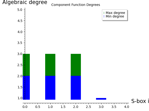
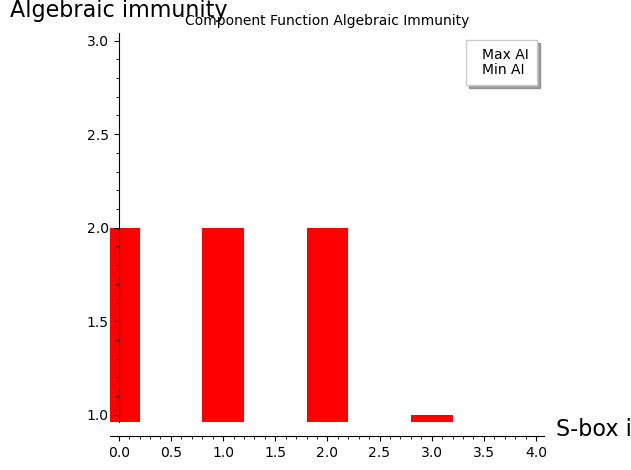
S-box         Min Deg  Max Deg   Min AI   Max AI
================================================
Heys                2        3        2        2
PRESENT             2        3        2        2
GIFT                2        3        2        2
Linear              1        1        1        1
# SageMath bar chart comparison
names = list(results.keys())
min_degs = [results[n]["min_deg"] for n in names]
max_degs = [results[n]["max_deg"] for n in names]
min_ais = [results[n]["min_ai"] for n in names]
max_ais = [results[n]["max_ai"] for n in names]

# Plot degree comparison
p1 = bar_chart(max_degs, width=0.4, color='green', legend_label='Max degree')
p1 += bar_chart(min_degs, width=0.4, color='blue', legend_label='Min degree')
p1.show(title="Component Function Degrees",
        axes_labels=["S-box index", "Algebraic degree"],
        ymax=n_bits + 1)

# Plot AI comparison
p2 = bar_chart(max_ais, width=0.4, color='orange', legend_label='Max AI')
p2 += bar_chart(min_ais, width=0.4, color='red', legend_label='Min AI')
p2.show(title="Component Function Algebraic Immunity",
        axes_labels=["S-box index", "Algebraic immunity"],
        ymax=3)
35.17 The AES S-Box (Conceptual)#
The AES S-box operates on 8-bit inputs, so it has \(2^8 = 256\) entries and each component function is a Boolean function on 8 variables. The AES S-box is defined as inversion in \(\text{GF}(2^8)\) followed by an affine transformation.
AES S-Box Properties
Algebraic degree: 7 (the maximum for a balanced 8-bit function).
Algebraic immunity: 3 (below the optimum of 4).
The inverse map \(x \mapsto x^{-1}\) in \(\text{GF}(2^8)\) can be written as \(x^{254}\) (since \(x^{255} = 1\) for all \(x \neq 0\)).
The ANF of each coordinate function has 255 terms out of a possible 256 – it is almost maximally complex.
Each S-box application produces 39 quadratic equations in 16 variables (Courtois and Pieprzyk, 2002).
Despite the high degree and term count, the specific algebraic structure of inversion in \(\text{GF}(2^8)\) gives rise to overdefined systems of quadratic equations when the S-box is modeled implicitly. This is the foundation of the XSL attack.
# AES S-box (standard FIPS 197 table)
AES_SBOX = [
    0x63, 0x7c, 0x77, 0x7b, 0xf2, 0x6b, 0x6f, 0xc5,
    0x30, 0x01, 0x67, 0x2b, 0xfe, 0xd7, 0xab, 0x76,
    0xca, 0x82, 0xc9, 0x7d, 0xfa, 0x59, 0x47, 0xf0,
    0xad, 0xd4, 0xa2, 0xaf, 0x9c, 0xa4, 0x72, 0xc0,
    0xb7, 0xfd, 0x93, 0x26, 0x36, 0x3f, 0xf7, 0xcc,
    0x34, 0xa5, 0xe5, 0xf1, 0x71, 0xd8, 0x31, 0x15,
    0x04, 0xc7, 0x23, 0xc3, 0x18, 0x96, 0x05, 0x9a,
    0x07, 0x12, 0x80, 0xe2, 0xeb, 0x27, 0xb2, 0x75,
    0x09, 0x83, 0x2c, 0x1a, 0x1b, 0x6e, 0x5a, 0xa0,
    0x52, 0x3b, 0xd6, 0xb3, 0x29, 0xe3, 0x2f, 0x84,
    0x53, 0xd1, 0x00, 0xed, 0x20, 0xfc, 0xb1, 0x5b,
    0x6a, 0xcb, 0xbe, 0x39, 0x4a, 0x4c, 0x58, 0xcf,
    0xd0, 0xef, 0xaa, 0xfb, 0x43, 0x4d, 0x33, 0x85,
    0x45, 0xf9, 0x02, 0x7f, 0x50, 0x3c, 0x9f, 0xa8,
    0x51, 0xa3, 0x40, 0x8f, 0x92, 0x9d, 0x38, 0xf5,
    0xbc, 0xb6, 0xda, 0x21, 0x10, 0xff, 0xf3, 0xd2,
    0xcd, 0x0c, 0x13, 0xec, 0x5f, 0x97, 0x44, 0x17,
    0xc4, 0xa7, 0x7e, 0x3d, 0x64, 0x5d, 0x19, 0x73,
    0x60, 0x81, 0x4f, 0xdc, 0x22, 0x2a, 0x90, 0x88,
    0x46, 0xee, 0xb8, 0x14, 0xde, 0x5e, 0x0b, 0xdb,
    0xe0, 0x32, 0x3a, 0x0a, 0x49, 0x06, 0x24, 0x5c,
    0xc2, 0xd3, 0xac, 0x62, 0x91, 0x95, 0xe4, 0x79,
    0xe7, 0xc8, 0x37, 0x6d, 0x8d, 0xd5, 0x4e, 0xa9,
    0x6c, 0x56, 0xf4, 0xea, 0x65, 0x7a, 0xae, 0x08,
    0xba, 0x78, 0x25, 0x2e, 0x1c, 0xa6, 0xb4, 0xc6,
    0xe8, 0xdd, 0x74, 0x1f, 0x4b, 0xbd, 0x8b, 0x8a,
    0x70, 0x3e, 0xb5, 0x66, 0x48, 0x03, 0xf6, 0x0e,
    0x61, 0x35, 0x57, 0xb9, 0x86, 0xc1, 0x1d, 0x9e,
    0xe1, 0xf8, 0x98, 0x11, 0x69, 0xd9, 0x8e, 0x94,
    0x9b, 0x1e, 0x87, 0xe9, 0xce, 0x55, 0x28, 0xdf,
    0x8c, 0xa1, 0x89, 0x0d, 0xbf, 0xe6, 0x42, 0x68,
    0x41, 0x99, 0x2d, 0x0f, 0xb0, 0x54, 0xbb, 0x16,
]

# Compute degree of each coordinate function of the AES S-box
B8.<z0,z1,z2,z3,z4,z5,z6,z7> = BooleanPolynomialRing(8)

print("Algebraic degree of AES S-box coordinate functions:")
print("=" * 50)
for bit in range(8):
    tt = [(AES_SBOX[xx] >> bit) & 1 for xx in range(256)]
    poly = truth_table_to_anf_sage(tt, B8)
    n_terms = len(poly.monomials())
    print(f"  Bit {bit}: degree = {poly.degree()}, active terms = {n_terms}/256")
Algebraic degree of AES S-box coordinate functions:
==================================================
  Bit 0: degree = 7, active terms = 132/256
  Bit 1: degree = 7, active terms = 133/256
  Bit 2: degree = 7, active terms = 145/256
  Bit 3: degree = 7, active terms = 136/256
  Bit 4: degree = 7, active terms = 131/256
  Bit 5: degree = 7, active terms = 114/256
  Bit 6: degree = 7, active terms = 112/256
  Bit 7: degree = 7, active terms = 110/256
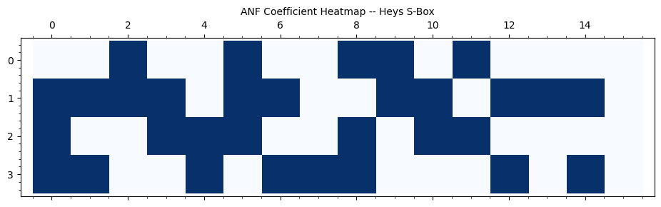
35.18 ANF Term Density Visualization#
We visualize which monomials appear in each coordinate function of the Heys S-box by plotting the ANF coefficient matrix.
# Build ANF matrix: rows = output bits, cols = monomial indices
anf_matrix = matrix(ZZ, n_bits, N)
for bit in range(n_bits):
    tt = [(SBOX_TABLE[xx] >> bit) & 1 for xx in range(N)]
    # Compute ANF coefficients via Mobius transform
    anf_coeffs = list(tt)
    for i in range(n_bits):
        stride = 1 << i
        for j in range(N):
            if j & stride:
                anf_coeffs[j] = (anf_coeffs[j] + anf_coeffs[j ^^ stride]) % 2
    for j in range(N):
        anf_matrix[bit, j] = anf_coeffs[j]

# Display as a matrix plot
matrix_plot(anf_matrix, cmap='Blues').show(
    title="ANF Coefficient Heatmap -- Heys S-Box",
    figsize=(12, 3)
)

# Print monomial labels
var_names = ["x0", "x1", "x2", "x3"]
print("Monomial mapping:")
for u in range(N):
    if u == 0:
        label = "1"
    else:
        factors = [var_names[i] for i in range(n_bits) if (u >> i) & 1]
        label = "*".join(factors)
    active = [bit for bit in range(n_bits) if anf_matrix[bit, u] == 1]
    if active:
        print(f"  u={int(u):2d} -> {label:12s}  active in y{active}")

total_terms = sum(anf_matrix.list())
max_terms = n_bits * N
print(f"\nTotal active terms: {total_terms}/{max_terms} "
      f"({float(100*total_terms/max_terms):.1f}%)")
Monomial mapping:
  u= 0 -> 1             active in y[1, 2, 3]
  u= 1 -> x0            active in y[1, 3]
  u= 2 -> x1            active in y[0, 1]
  u= 3 -> x0*x1         active in y[1, 2]
  u= 4 -> x2            active in y[2, 3]
  u= 5 -> x0*x2         active in y[0, 1, 2]
  u= 6 -> x1*x2         active in y[1, 3]
  u= 7 -> x0*x1*x2      active in y[3]
  u= 8 -> x3            active in y[0, 2, 3]
  u= 9 -> x0*x3         active in y[0, 1]
  u=10 -> x1*x3         active in y[1, 2]
  u=11 -> x0*x1*x3      active in y[0, 2]
  u=12 -> x2*x3         active in y[1, 3]
  u=13 -> x0*x2*x3      active in y[1]
  u=14 -> x1*x2*x3      active in y[1, 3]

Total active terms: 31/64 (48.4%)
35.19 Degree Growth Through S-Box Composition#
When S-boxes are composed (as in multiple rounds of a cipher), the algebraic degree of the resulting function grows. For a single S-box of degree \(d\) applied \(r\) times, the degree can grow up to \(d^r\) (bounded by \(2^n - 1\)). Let us measure this experimentally.
max_rounds = 8

# Compose the S-box with itself r times and measure degree
round_degrees = []

for r in range(1, max_rounds + 1):
    composed = list(range(N))
    for _ in range(r):
        composed = [SBOX_TABLE[composed[xx]] for xx in range(N)]

    degs = []
    for bit in range(n_bits):
        tt = [(composed[xx] >> bit) & 1 for xx in range(N)]
        poly = truth_table_to_anf_sage(tt, B)
        degs.append(poly.degree())
    round_degrees.append(degs)

# Plot using SageMath
rounds = list(range(1, max_rounds + 1))
colors = ['blue', 'green', 'red', 'purple']
p = Graphics()
for bit in range(n_bits):
    degs_for_bit = [round_degrees[r][bit] for r in range(max_rounds)]
    p += list_plot(list(zip(rounds, degs_for_bit)), plotjoined=True,
                   color=colors[bit], marker='o', legend_label=f'y{bit}',
                   thickness=2)
p += line([(1, n_bits - 1), (max_rounds, n_bits - 1)],
          color='red', linestyle='--', alpha=0.5, legend_label=f'Max degree = {n_bits-1}')
p.show(title="Degree Growth Under S-Box Composition",
       axes_labels=["Number of compositions", "Algebraic degree"])

# Print table
print(f"{'Round':>6}  {'y0':>4} {'y1':>4} {'y2':>4} {'y3':>4}  {'max':>4}")
print("-" * 35)
for r, degs in enumerate(round_degrees, 1):
    print(f"{r:>6}  {degs[0]:>4} {degs[1]:>4} {degs[2]:>4} {degs[3]:>4}  {max(degs):>4}")
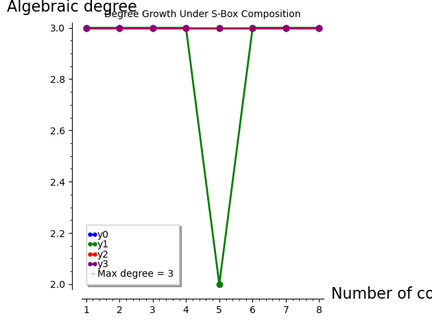
 Round    y0   y1   y2   y3   max
-----------------------------------
     1     3    3    3    3     3
     2     3    3    3    3     3
     3     3    3    3    3     3
     4     3    3    3    3     3
     5     3    2    3    3     3
     6     3    3    3    3     3
     7     3    3    3    3     3
     8     3    3    3    3     3
Degree Saturation
The degree quickly saturates at 3 (the maximum for a balanced 4-bit permutation). In a real cipher, key addition between rounds prevents simple composition, but the degree growth still tells us that after a few rounds, the algebraic expressions become very complex – this is the cipher’s defense against algebraic attacks.
35.20 Monomial Count Growth#
Another indicator of algebraic complexity is how the number of active monomials in the ANF grows with the number of S-box compositions.
round_counts = []
for r in range(1, max_rounds + 1):
    composed = list(range(N))
    for _ in range(r):
        composed = [SBOX_TABLE[composed[xx]] for xx in range(N)]

    total_terms = 0
    for bit in range(n_bits):
        tt = [(composed[xx] >> bit) & 1 for xx in range(N)]
        poly = truth_table_to_anf_sage(tt, B)
        total_terms += len(poly.monomials())
    round_counts.append(total_terms)

# SageMath bar chart
p = bar_chart(round_counts, color='#76b7b2', width=0.7)
p += line([(0, n_bits * N), (max_rounds, n_bits * N)],
          color='red', linestyle='--', alpha=0.5, legend_label=f'Max possible = {n_bits * N}')
p.show(title="Monomial Count Growth Under Composition",
       axes_labels=["Number of compositions", "Total active ANF monomials (all 4 bits)"])

for r, c in enumerate(round_counts, 1):
    print(f"  Round {r}: {c}/{n_bits*N} terms ({float(100*c/(n_bits*N)):.1f}%)")
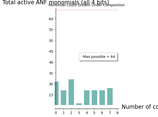
  Round 1: 31/64 terms (48.4%)
  Round 2: 27/64 terms (42.2%)
  Round 3: 32/64 terms (50.0%)
  Round 4: 21/64 terms (32.8%)
  Round 5: 27/64 terms (42.2%)
  Round 6: 27/64 terms (42.2%)
  Round 7: 27/64 terms (42.2%)
  Round 8: 28/64 terms (43.8%)
35.21 Exercises#
Exercise 35.1 (ANF by hand)
Compute the ANF of the Boolean function \(f : \text{GF}(2)^3 \to \text{GF}(2)\) with truth table \((0, 1, 1, 0, 1, 0, 0, 1)\). What is its algebraic degree?
Hint
Apply the Mobius transform: for each index \(u\), compute \(a_u = \bigoplus_{v \preceq u} f(v)\), where \(v \preceq u\) means that every bit of \(v\) is \(\leq\) the corresponding bit of \(u\). The degree equals the maximum Hamming weight among indices with \(a_u = 1\). This particular truth table is the 3-variable XOR function \(x_0 \oplus x_1 \oplus x_2\).
Exercise 35.2 (Affine functions)
Prove that a Boolean function has algebraic degree \(\leq 1\) if and only if it is affine (i.e., \(f(x) = a_0 \oplus a_1 x_1 \oplus \cdots \oplus a_n x_n\)). Why are affine S-boxes catastrophically insecure?
Hint
Degree \(\leq 1\) means the ANF has no monomials of degree 2 or higher, so \(f\) is a linear combination of variables plus a constant – this is exactly the definition of affine. An affine S-box means the entire cipher is a system of linear equations over \(\text{GF}(2)\), solvable by Gaussian elimination with a single known plaintext–ciphertext pair.
Exercise 35.3 (Groebner basis attack on the toy SPN)
Modify the SPN to use a different S-box permutation (e.g.,
perm = [3, 1, 6, 4, 7, 5, 2, 0]) and repeat the elimination ideal
analysis. Does the new S-box still have key-independent output bits?
Compute the percentage of plaintext candidates eliminated with
knowledge of \((k_4, k_5)\) and one ciphertext.
Hint
Follow the same workflow: compute Spol0, Spol1, Spol2 for the
new S-box, rebuild SBoxModel, set up the coordinate ring and
quotient ring, and compute relI.elimination_ideal([k0,...,k5]).
A well-designed S-box should yield a trivial elimination ideal
(just \(\langle 0 \rangle\)).
Exercise 35.4 (Annihilators via Groebner bases)
Find a nonzero Boolean function \(g\) on 4 variables such that
\(f \cdot g = 0\), where \(f\) is the output bit \(y_0\) of the Heys S-box.
Use SageMath’s ideal and groebner_basis to find \(g\).
Hint
The support of \(y_0\) (where it equals 1) has 8 elements. Set up
the polynomial ring BooleanPolynomialRing(4, 'x') and form
the vanishing ideal of the support points. Any element of degree
\(\leq 2\) in this ideal is an annihilator of \(f\).
Exercise 35.5 (Scaling analysis)
For the 3-round SPN with \(n\)-bit S-boxes and a block size of \(4n\) bits (four S-boxes per round), derive formulas for the number of variables and equations as a function of \(n\). At what value of \(n\) does the system become underdefined (more variables than equations)?
Hint
Use the counting approach from Section 35.12. The key observation is that the number of field equations grows linearly with the number of variables, while the ANF equations grow with the number of S-box applications times \(n\). Since each S-box application also introduces \(2n\) new variables but only \(n\) ANF equations, larger S-boxes tend to produce underdefined systems unless additional equations (e.g., from multiple plaintext–ciphertext pairs) are added.
35.22 Summary#
In this chapter we used SageMath’s algebraic machinery to perform a complete algebraic cryptanalysis of an SPN cipher.
Key takeaways:
Every Boolean function has a unique ANF, and SageMath can compute it symbolically using
PolynomialRing(GF(2), ...)and Groebner bases.Groebner bases over \(\text{GF}(2)\) with Boolean field equations (\(v_i^2 - v_i = 0\)) effectively solve polynomial systems, yielding the algebraic variety of solutions.
Elimination ideals reveal which plaintext-ciphertext relations are independent of the key – a catastrophic structural weakness in our toy SPN.
With knowledge of just 2 out of 6 key bits and one ciphertext, the algebraic attack eliminates approximately 70% of plaintext candidates.
The algebraic degree measures the complexity of the polynomial representation. Higher degree makes algebraic attacks harder. The Heys S-box achieves the optimal degree of 3 for all component functions.
The algebraic immunity measures resistance to annihilator-based attacks. The Heys S-box achieves the optimal value of 2 for \(n = 4\).
SageMath tools used:
GF(2),PolynomialRing,BooleanPolynomialRing,ideal(),.groebner_basis(),.elimination_ideal(),AffineSpace,.subscheme(),.irreducible_components(),.rational_points(),SymmetricGroup,PermutationGroupElement.
References:
G. V. Bard, Algebraic Cryptanalysis, Springer, 2009.
N. T. Courtois and J. Pieprzyk, “Cryptanalysis of Block Ciphers with Overdefined Systems of Equations,” ASIACRYPT 2002.
N. T. Courtois and G. V. Bard, “Algebraic Cryptanalysis of the Data Encryption Standard,” IMA 2007.
C. Carlet, Boolean Functions for Cryptography and Coding Theory, Cambridge University Press, 2021.
M. S. E. Mohamed, W. S. A. E. Mohamed, J. Ding, and J. Buchmann, “MXL2: Solving Polynomial Equations over GF(2) Using an Improved Mutant Strategy,” PQCrypto 2008.