Chapter 45: Synthesis — From Al-Kindi to Post-Quantum

Chapter 45: Synthesis — From Al-Kindi to Post-Quantum#

This final chapter synthesises the entire arc of Elements of Cryptanalysis. We trace the discipline from its origins in ninth-century Baghdad to the post-quantum frontier, drawing out the recurring patterns, key themes, and open problems that define the field today.

45.1 A Timeline of Cryptanalysis (850 AD – 2024)#

Cryptanalysis has evolved through several distinct eras. The visualisation below places landmark events on a logarithmic-feel timeline that compresses the long pre-modern period while expanding the rapid developments of the twentieth and twenty-first centuries.

Show code cell source Hide code cell source

import numpy as np
import matplotlib.pyplot as plt

# --- Landmark events in the history of cryptanalysis ---
events = [
    (850,  "Al-Kindi's frequency\nanalysis manuscript"),
    (1467, "Alberti's polyalphabetic\ncipher disk"),
    (1586, "Babington Plot —\ncipher broken"),
    (1863, "Kasiski examination\nof Vigenère"),
    (1917, "Zimmermann Telegram\ndecrypted"),
    (1932, "Rejewski breaks\nEnigma"),
    (1943, "Colossus at\nBletchley Park"),
    (1949, "Shannon's Communication\nTheory of Secrecy"),
    (1976, "Diffie-Hellman\nkey exchange"),
    (1977, "RSA public-key\ncryptosystem"),
    (1990, "Differential\ncryptanalysis (Biham-Shamir)"),
    (1993, "Linear cryptanalysis\n(Matsui)"),
    (1994, "Shor's quantum\nfactoring algorithm"),
    (2001, "AES adopted\nas standard"),
    (2009, "Lattice-based\ncrypto advances"),
    (2017, "NIST PQC\nstandardisation begins"),
    (2022, "CRYSTALS-Kyber &\nDilithium selected"),
    (2024, "Code-based & isogeny\nfrontiers active"),
]

years = [e[0] for e in events]
labels = [e[1] for e in events]

fig, ax = plt.subplots(figsize=(16, 9))

# Colour-code by era
colours = []
for y in years:
    if y < 1800:
        colours.append('#8B4513')   # Classical era — brown
    elif y < 1940:
        colours.append('#2E8B57')   # Early modern — green
    elif y < 1976:
        colours.append('#4169E1')   # Mid-century — blue
    elif y < 2000:
        colours.append('#9932CC')   # Public-key era — purple
    else:
        colours.append('#DC143C')   # Post-quantum era — crimson

# Plot stems
for i, (y, lbl) in enumerate(events):
    side = 1 if i % 2 == 0 else -1
    height = side * (0.6 + 0.25 * (i % 3))
    ax.plot([y, y], [0, height], color=colours[i], linewidth=1.5, zorder=2)
    ax.scatter(y, 0, color=colours[i], s=60, zorder=3)
    ax.text(y, height + side * 0.08, lbl, ha='center',
            va='bottom' if side > 0 else 'top',
            fontsize=7.5, color=colours[i], fontweight='bold')

# Central axis
ax.axhline(0, color='grey', linewidth=1.0, zorder=1)

# Era shading
era_spans = [
    (800, 1800, '#8B4513', 'Classical'),
    (1800, 1940, '#2E8B57', 'Mechanised'),
    (1940, 1976, '#4169E1', 'Information Age'),
    (1976, 2000, '#9932CC', 'Public-Key'),
    (2000, 2030, '#DC143C', 'Post-Quantum'),
]
for start, end, col, name in era_spans:
    ax.axvspan(start, end, alpha=0.06, color=col)
    ax.text((start + end) / 2, -1.25, name, ha='center', fontsize=9,
            color=col, fontstyle='italic')

ax.set_xlim(800, 2035)
ax.set_ylim(-1.5, 1.5)
ax.set_xlabel('Year', fontsize=12)
ax.set_title('A Timeline of Cryptanalysis — 850 AD to 2024',
             fontsize=14, fontweight='bold')
ax.set_yticks([])
ax.spines['left'].set_visible(False)
ax.spines['right'].set_visible(False)
ax.spines['top'].set_visible(False)

plt.tight_layout()
plt.savefig('fig_ch45_timeline.png', dpi=150, bbox_inches='tight')
plt.show()

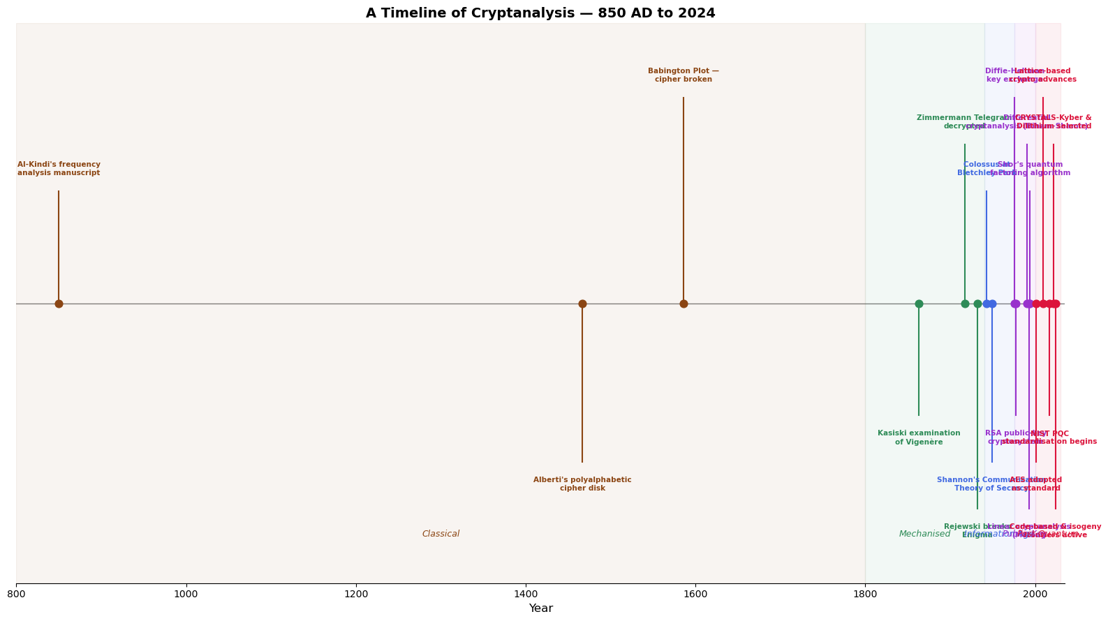
../_images/4ad0d519e390a5528877cc466b16134435ee7693d84a283f1a3c667e89464b4a.png

Historical Note

Al-Kindi’s Risalah fi Istikhraj al-Mu’amma (c. 850 AD) is the earliest known treatise on cryptanalysis. His frequency-analysis technique remained the dominant attack strategy for over 600 years — an extraordinary reign in any technical discipline.

45.2 The Recurring Pattern: Cipher → Attack → Stronger Cipher#

Throughout the history of cryptography, a single dialectical pattern has repeated itself with striking regularity:

A cipher is proposed, believed secure.
An attack reveals a structural weakness.
A stronger cipher is designed in response, informed by the nature of the attack.

This evolutionary arms race is the engine that drives cryptographic progress.

Show code cell source Hide code cell source

import numpy as np
import matplotlib.pyplot as plt

# Cipher-Attack-Response triples
triples = [
    ('Caesar / Mono-\nalphabetic', 'Frequency\nAnalysis', 'Polyalphabetic\nCiphers'),
    ('Vigenère\nCipher', 'Kasiski /\nIC Analysis', 'Rotor\nMachines'),
    ('Enigma', 'Bomba /\nBanburismus', 'One-Time Pad\n(theory)'),
    ('DES', 'Differential &\nLinear Crypt.', 'AES / Modern\nBlock Ciphers'),
    ('RSA / DH', "Shor's\nAlgorithm", 'Lattice / Code-\nBased Crypto'),
]

fig, ax = plt.subplots(figsize=(14, 7))

n = len(triples)
y_positions = np.arange(n)[::-1] * 1.5

box_w = 2.0
col_cipher = 0.0
col_attack = 4.5
col_response = 9.0

cipher_color = '#3274A1'
attack_color = '#E1812C'
response_color = '#3A923A'

for i, (cipher, attack, response) in enumerate(triples):
    y = y_positions[i]

    # Boxes
    for x, label, color in [(col_cipher, cipher, cipher_color),
                             (col_attack, attack, attack_color),
                             (col_response, response, response_color)]:
        rect = plt.Rectangle((x - box_w/2, y - 0.45), box_w, 0.9,
                             facecolor=color, alpha=0.15, edgecolor=color,
                             linewidth=2, zorder=2)
        ax.add_patch(rect)
        ax.text(x, y, label, ha='center', va='center', fontsize=8.5,
                fontweight='bold', color=color, zorder=3)

    # Arrows
    ax.annotate('', xy=(col_attack - box_w/2 - 0.1, y),
                xytext=(col_cipher + box_w/2 + 0.1, y),
                arrowprops=dict(arrowstyle='->', color='grey', lw=1.5))
    ax.annotate('', xy=(col_response - box_w/2 - 0.1, y),
                xytext=(col_attack + box_w/2 + 0.1, y),
                arrowprops=dict(arrowstyle='->', color='grey', lw=1.5))

    # Feedback loop (response feeds next cipher)
    if i < n - 1:
        y_next = y_positions[i + 1]
        ax.annotate('', xy=(col_cipher + box_w/2, y_next + 0.45),
                    xytext=(col_response + box_w/2, y - 0.45),
                    arrowprops=dict(arrowstyle='->', color='#AAAAAA',
                                   lw=1.0, linestyle='--',
                                   connectionstyle='arc3,rad=0.3'))

# Column headers
header_y = y_positions[0] + 1.2
for x, label, color in [(col_cipher, 'CIPHER', cipher_color),
                          (col_attack, 'ATTACK', attack_color),
                          (col_response, 'STRONGER CIPHER', response_color)]:
    ax.text(x, header_y, label, ha='center', va='center', fontsize=12,
            fontweight='bold', color=color)

ax.set_xlim(-2, 12)
ax.set_ylim(-1.5, header_y + 0.8)
ax.set_aspect('equal')
ax.axis('off')
ax.set_title('The Dialectic of Cryptanalysis: Cipher → Attack → Stronger Cipher',
             fontsize=13, fontweight='bold', pad=15)

plt.tight_layout()
plt.savefig('fig_ch45_dialectic.png', dpi=150, bbox_inches='tight')
plt.show()

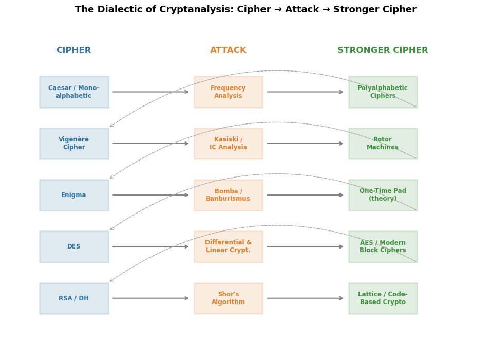
../_images/f414ff2d2b761e6426d8c6ceaedf834e6a9eeb102d6b2ccb4005e11c33e5777c.png

Key Insight

Every successful attack has made cryptography stronger, not weaker. Differential cryptanalysis did not destroy block ciphers — it led to the design of AES with provable resistance to such attacks. Shor’s algorithm has not destroyed public-key cryptography — it has catalysed the development of post-quantum schemes.

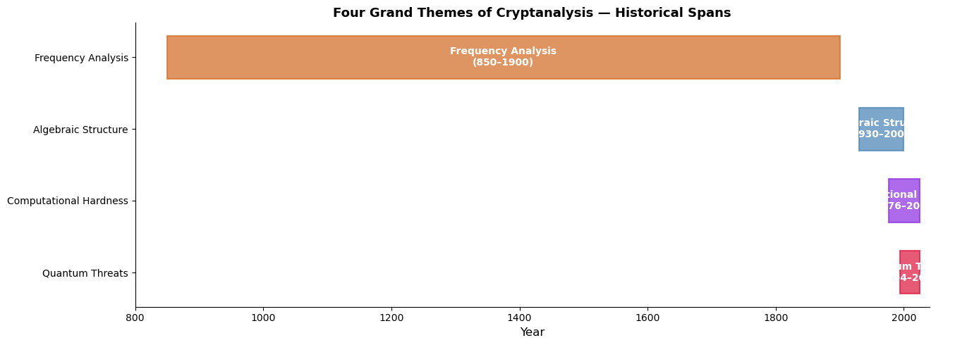
45.3 Key Themes Across the Course#

Four grand themes emerge from our study:

Theme	Era	Central Idea
Frequency Analysis	Classical (850–1800s)	Natural-language statistics reveal plaintext
Algebraic Structure	Mechanical/Modern (1930s–1990s)	Exploiting mathematical structure in ciphers
Computational Hardness	Public-Key (1976–present)	Security rests on presumed intractable problems
Quantum Threats	Post-Quantum (1994–present)	Quantum computers break hardness assumptions

../_images/509deac0f757fd5561f6be4290cb8cebe76a8babc598e2ce4cce28b411a6c601.png

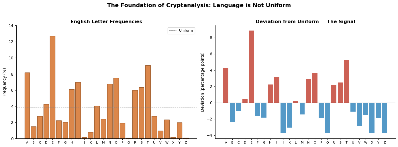
45.3.1 Theme 1: Frequency Analysis#

The insight that human language is not uniform — that certain letters, digrams, and patterns recur with predictable frequencies — was the first great weapon of the cryptanalyst. Al-Kindi formalised it, and it remained dominant for centuries. Even modern attacks on stream ciphers echo this idea: any deviation from uniform randomness is a potential vulnerability.

../_images/d171d7b1e46e40ab1e434264ca100996dbd11c81855cd4ec8f6b159cd838878c.png

45.3.2 Theme 2: Algebraic Structure#

The twentieth century brought the realisation that ciphers are mathematical objects whose structure can be analysed algebraically. Rejewski modelled the Enigma permutations as group elements. Differential and linear cryptanalysis exploit the algebraic properties of S-boxes. The shift from “art” to “science” in cryptanalysis was, at its heart, the shift toward algebraic thinking.

45.3.3 Theme 3: Computational Hardness#

With the advent of public-key cryptography in 1976, security became explicitly linked to computational hardness assumptions: integer factorisation, discrete logarithms, and later lattice problems. The cryptanalyst’s task transformed from finding the key to finding an efficient algorithm for a hard problem — or proving that none exists.

45.3.4 Theme 4: Quantum Threats#

Shor’s 1994 algorithm demonstrated that quantum computers could efficiently solve factoring and discrete logarithms — the very problems underpinning RSA, DSA, and elliptic curve cryptography. This existential threat has driven the development of post-quantum cryptography based on lattices, codes, hash functions, isogenies, and multivariate equations.

../_images/c0eedda251f9105d4c34fc6e7538f52a23b78cf19a7d105cb3cd3dfdf42fdfbe.png

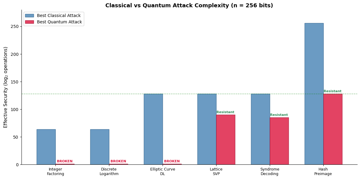
Why Post-Quantum Matters Now

Even though large-scale quantum computers do not yet exist, the “harvest now, decrypt later” threat means that adversaries can store encrypted traffic today and decrypt it once quantum computers become available. Migration to post-quantum cryptography is therefore urgent.

45.4 Open Problems in Cryptanalysis#

The field remains vibrantly open. Below we catalogue the most significant unsolved questions, organised by domain.

../_images/5ffe4c8bd218171457ec39814245fa5c599fa98ef221ee9ac6e7b0da9f86c1f7.png

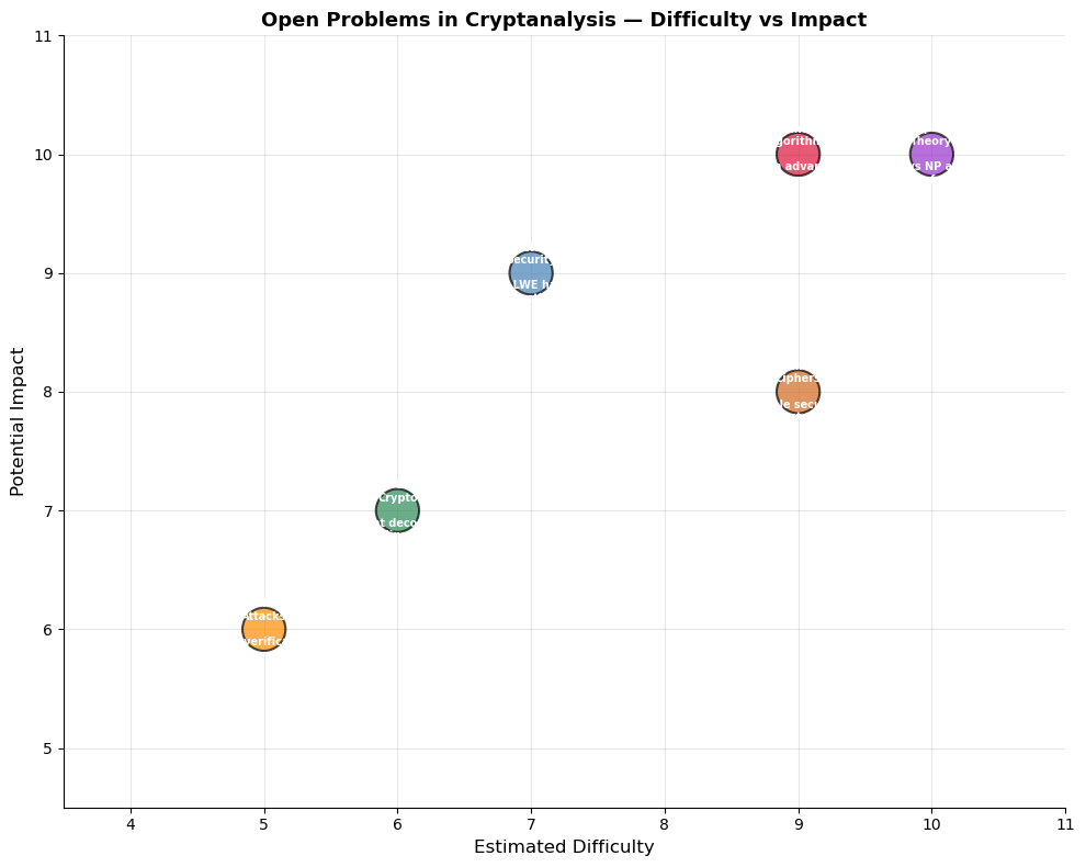
The Deepest Open Problem

The question of whether one-way functions exist — intimately connected to the P vs NP problem — remains the deepest open question in cryptography. If P = NP, then no computationally-secure cryptography is possible (except information-theoretic schemes like the one-time pad). Nearly all of modern cryptography rests on the assumption that P ≠ NP.

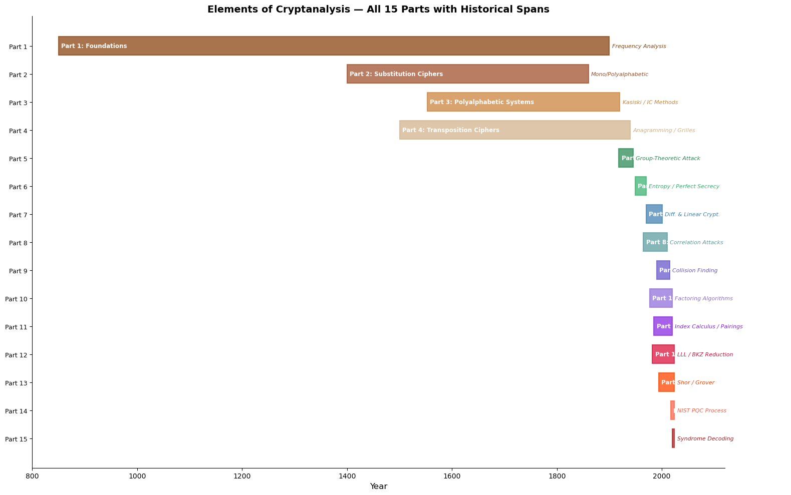
45.5 Summary of All 15 Parts#

The following table and visualisation summarise the full course structure, mapping each part to its key technique, approximate historical period, and primary impact on the field.

Show code cell source Hide code cell source

import numpy as np
import matplotlib.pyplot as plt

# Full course summary data
parts = [
    ('Part 1',  'Foundations',                     'Frequency Analysis',        850,  1900, '#8B4513'),
    ('Part 2',  'Substitution Ciphers',            'Mono/Polyalphabetic',       1400, 1860, '#A0522D'),
    ('Part 3',  'Polyalphabetic Systems',           'Kasiski / IC Methods',      1553, 1920, '#CD853F'),
    ('Part 4',  'Transposition Ciphers',            'Anagramming / Grilles',     1500, 1940, '#D2B48C'),
    ('Part 5',  'Rotor Machines',                   'Group-Theoretic Attack',    1918, 1945, '#2E8B57'),
    ('Part 6',  'Shannon & Information Theory',     'Entropy / Perfect Secrecy', 1949, 1970, '#3CB371'),
    ('Part 7',  'Block Ciphers',                    'Diff. & Linear Crypt.',     1970, 2001, '#4682B4'),
    ('Part 8',  'Stream Ciphers',                   'Correlation Attacks',       1965, 2010, '#5F9EA0'),
    ('Part 9',  'Hash Functions',                   'Collision Finding',         1990, 2015, '#6A5ACD'),
    ('Part 10', 'Public-Key: RSA',                  'Factoring Algorithms',      1977, 2020, '#9370DB'),
    ('Part 11', 'Elliptic Curves',                  'Index Calculus / Pairings', 1985, 2020, '#8A2BE2'),
    ('Part 12', 'Algebraic Cryptanalysis',          'Gröbner Bases / ANF',       2000, 2024, '#DC143C'),
    ('Part 13', 'The Quantum Threat',               "Shor / Grover",             1994, 2024, '#FF4500'),
    ('Part 14', 'Lattice-Based Cryptography',       'LLL / BKZ Reduction',       1982, 2024, '#FF6347'),
    ('Part 15', 'Code-Based & Frontiers',           'Syndrome Decoding / PQC',   2017, 2024, '#B22222'),
]

fig, ax = plt.subplots(figsize=(16, 10))

for i, (part, title, technique, start, end, color) in enumerate(parts):
    y = len(parts) - 1 - i
    ax.barh(y, end - start, left=start, height=0.65, color=color,
            alpha=0.75, edgecolor=color, linewidth=1.5)
    ax.text(start + 5, y, f'{part}: {title}', va='center', fontsize=8.5,
            fontweight='bold', color='white')
    ax.text(end + 5, y, technique, va='center', fontsize=8, color=color,
            fontstyle='italic')

ax.set_yticks(range(len(parts)))
ax.set_yticklabels([p[0] for p in parts][::-1], fontsize=9)
ax.set_xlabel('Year', fontsize=12)
ax.set_title('Elements of Cryptanalysis — All 15 Parts with Historical Spans',
             fontsize=14, fontweight='bold')
ax.set_xlim(800, 2120)
ax.spines['top'].set_visible(False)
ax.spines['right'].set_visible(False)

plt.tight_layout()
plt.savefig('fig_ch45_all_parts.png', dpi=150, bbox_inches='tight')
plt.show()

../_images/100c0fc12abad883c55fdd48b4b7a34cc4b4d0bcb67d50324d65a787f14ec084.png

Complete Course Summary Table#

Part	Title	Key Technique	Period	Impact
1	Foundations	Frequency analysis	850–1900	Birth of cryptanalysis as a discipline
2	Substitution Ciphers	Mono/polyalphabetic analysis	1400–1860	Broke centuries of “secure” communication
3	Polyalphabetic Systems	Kasiski / Index of Coincidence	1553–1920	Defeated the “indecipherable” Vigenère
4	Transposition Ciphers	Anagramming, grille analysis	1500–1940	Revealed permutation vulnerabilities
5	Rotor Machines	Group-theoretic cycle analysis	1918–1945	Changed the course of World War II
6	Shannon & Information Theory	Entropy, unicity distance	1949–1970	Put cryptography on rigorous foundations
7	Block Ciphers	Differential & linear cryptanalysis	1970–2001	Shaped DES, led to AES design
8	Stream Ciphers	Correlation & algebraic attacks	1965–2010	Secured wireless and real-time comm.
9	Hash Functions	Collision finding, length extension	1990–2015	SHA-3 and sponge constructions
10	Public-Key: RSA	Factoring (NFS, ECM)	1977–2020	Foundation of e-commerce security
11	Elliptic Curves	Index calculus, pairing attacks	1985–2020	Efficient public-key at shorter key sizes
12	Algebraic Cryptanalysis	Gröbner bases, polynomial systems	2000–2024	Algebraic modeling of ciphers over GF(2)
13	The Quantum Threat	Shor’s and Grover’s algorithms	1994–2024	Existential threat to classical PKC
14	Lattice-Based Cryptography	LLL/BKZ basis reduction	1982–2024	Leading post-quantum candidate family
15	Code-Based Crypto & Frontiers	Syndrome decoding, NIST PQC	2017–2024	PQC standards and diversifying portfolio

45.6 The Security#

Landscape: A Quantitative View

We now quantify how the effective security of different cryptographic families has evolved over time, accounting for both classical and quantum improvements in attacks.

Show code cell source Hide code cell source

import numpy as np
import matplotlib.pyplot as plt

# Effective security (bits) of various 128-bit-target schemes over decades
decades = np.array([1970, 1980, 1990, 2000, 2010, 2020, 2030])
labels_decade = [str(y) for y in decades]

# Rough effective security trajectories
des_security    = np.array([56, 56, 48, 42, 40, 38, 36])
rsa1024         = np.array([np.nan, 100, 90, 80, 73, 65, 0])    # broken by quantum ~2030s
aes128          = np.array([np.nan, np.nan, np.nan, 128, 128, 128, 128])
ecc256          = np.array([np.nan, np.nan, 128, 128, 128, 128, 0])  # broken by Shor
lattice256      = np.array([np.nan, np.nan, np.nan, np.nan, np.nan, 128, 120])
code_based      = np.array([np.nan, np.nan, np.nan, np.nan, np.nan, 128, 125])

fig, ax = plt.subplots(figsize=(12, 7))

schemes = [
    (des_security, 'DES (56-bit)', '#FF6347', 's'),
    (rsa1024, 'RSA-1024', '#9370DB', 'o'),
    (aes128, 'AES-128', '#4682B4', '^'),
    (ecc256, 'ECC-256', '#2E8B57', 'D'),
    (lattice256, 'Lattice-256', '#DC143C', 'P'),
    (code_based, 'Code-Based', '#FF8C00', 'X'),
]

for data, label, color, marker in schemes:
    mask = ~np.isnan(data)
    ax.plot(decades[mask], data[mask], '-o', color=color, label=label,
            marker=marker, markersize=8, linewidth=2, alpha=0.8)

ax.axhline(128, color='green', linestyle='--', linewidth=1, alpha=0.5)
ax.text(1972, 130, '128-bit target', fontsize=9, color='green')

ax.axhline(80, color='orange', linestyle='--', linewidth=1, alpha=0.5)
ax.text(1972, 82, '80-bit minimum (legacy)', fontsize=9, color='orange')

# Quantum era shading
ax.axvspan(2025, 2035, alpha=0.08, color='red')
ax.text(2027, 10, 'Quantum\nEra?', fontsize=10, color='red', fontstyle='italic')

ax.set_xlabel('Decade', fontsize=12)
ax.set_ylabel('Effective Security (bits)', fontsize=12)
ax.set_title('Evolution of Effective Security Across Cryptographic Families',
             fontsize=13, fontweight='bold')
ax.legend(fontsize=9, loc='lower left')
ax.set_ylim(-5, 145)
ax.set_xlim(1965, 2035)
ax.spines['top'].set_visible(False)
ax.spines['right'].set_visible(False)
ax.grid(True, alpha=0.2)

plt.tight_layout()
plt.savefig('fig_ch45_security_evolution.png', dpi=150, bbox_inches='tight')
plt.show()

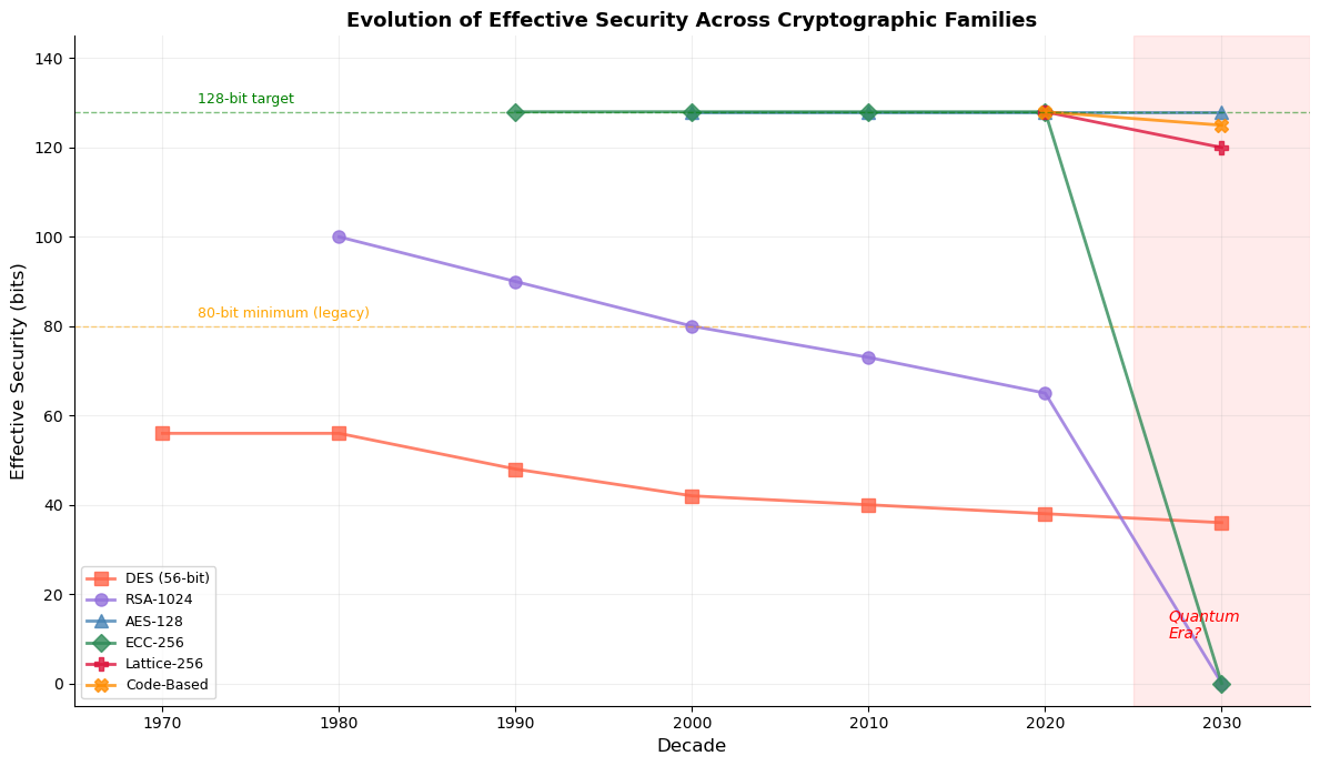
../_images/f01bbaa092d27ab819ca44857c6a3f705f59c3f09ac12fbbdaae5b93a7cf87e8.png

Interpreting the Security Evolution

The trajectories above are illustrative, not precise. The key message is that classical schemes degrade over time as attacks improve and hardware grows faster, while quantum-vulnerable schemes face a cliff-edge collapse. Post-quantum candidates (lattice, code-based) are designed to resist both classical and quantum attackers.

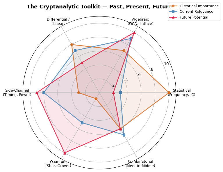
45.7 The Cryptanalytic Toolkit: A Taxonomy#

Over the course we have encountered dozens of attack techniques. The following radar chart groups them into six broad categories and estimates their relative importance in modern cryptanalysis.

../_images/611d5b7e7dd1b63155614b646d9e26f36febf321c4a1ebe62552095f1f5a5899.png

45.8 Lessons for the Practitioner#

From our survey, several practical lessons emerge:

Never rely on obscurity. Every proprietary cipher that has been analysed has been broken. Kerckhoffs’ principle (1883) remains paramount.
Understand your threat model. Classical, quantum, and side-channel attackers require different defences.
Crypto-agility is essential. Systems must be designed so that algorithms can be swapped without rebuilding the architecture.
Implementation matters as much as theory. Heartbleed, BEAST, and CRIME were all attacks on implementations, not on the underlying mathematics.
Diversity is a defence. Relying on a single hardness assumption (e.g., only lattices) is fragile. A portfolio approach — lattice, code-based, hash-based — provides resilience.

../_images/269c2093d2c7e3f932e00070592a6066cd7f6e324ff90b80153a51e9bca76baa.png

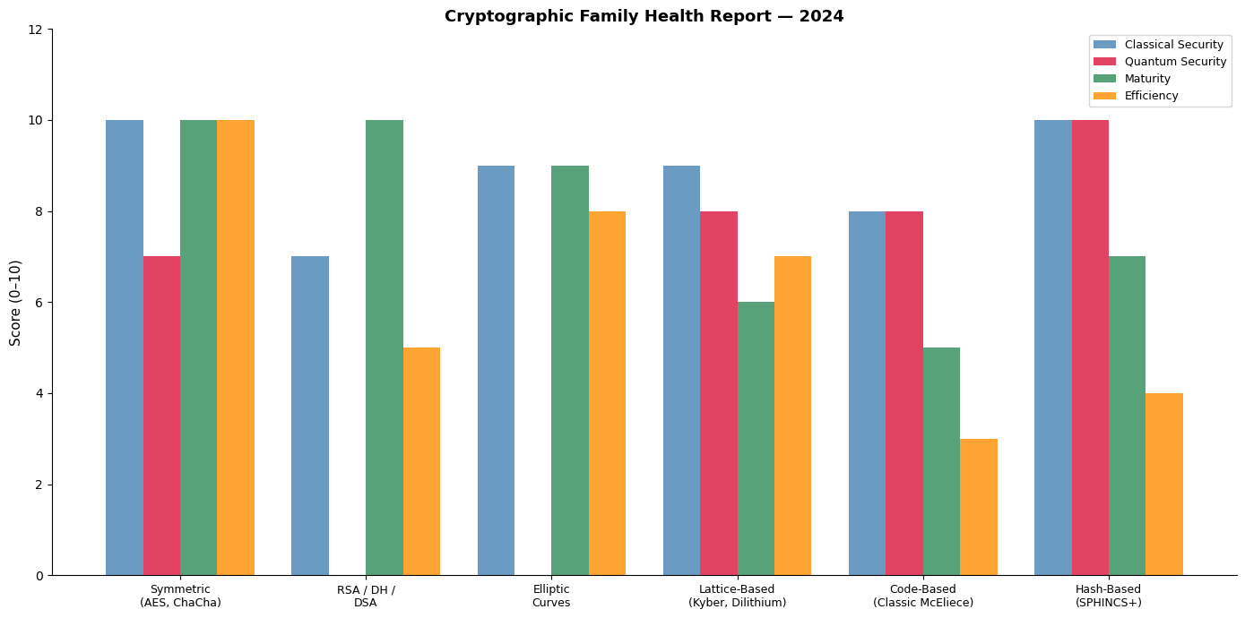
The Portfolio Approach

No single post-quantum family excels in all dimensions. NIST’s decision to standardise schemes from multiple families (lattice-based Kyber/Dilithium alongside hash-based SPHINCS+ and code-based candidates) reflects the wisdom of diversification — precisely because our confidence in any single hardness assumption is necessarily limited.

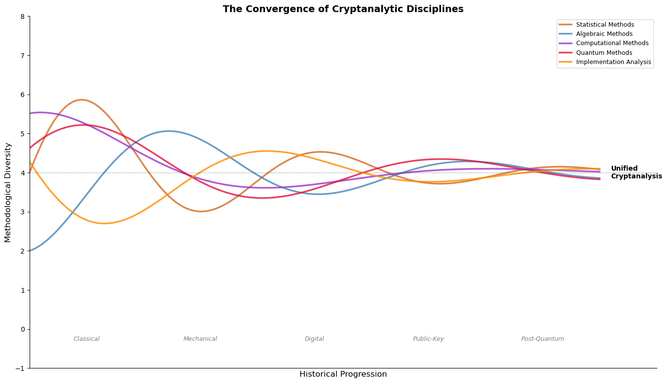
45.9 Concluding Reflections on the Future of Cryptography#

As we close this course, several forward-looking observations are worth recording.

The transition to post-quantum cryptography is underway. NIST has published its first post-quantum standards. The migration of the global internet to these new algorithms is a multi-decade infrastructure project comparable in scale to the transition from HTTP to HTTPS.

Cryptanalysis will continue to surprise us. The 2022 break of SIDH/SIKE — a leading isogeny-based candidate — by Castryck and Decru demonstrated that even well-studied schemes can fall to unexpected mathematical insights. Vigilance and scepticism remain the cryptanalyst’s chief virtues.

The interplay of theory and practice deepens. Formal verification, constant-time programming, and hardware-software co-design are becoming as important as the mathematical theory of the underlying algorithms. The cryptanalyst of the future must be as comfortable reading assembly code as proving theorems.

AI-assisted cryptanalysis is emerging. Machine learning techniques are beginning to be applied to cipher analysis, side-channel attacks, and protocol verification. Whether AI will produce fundamentally new attack paradigms — or merely accelerate existing ones — remains to be seen.

The human element persists. Despite all mathematical and computational advances, the weakest link in most cryptographic systems remains the human user. Social engineering, key mismanagement, and implementation errors continue to dominate real-world breaches.

../_images/a0efe75d72b6314b7811b9dd349c8e1f662df36bd0e9223ed7d87c799f9448fb.png

A Final Word

Cryptanalysis is not merely the art of breaking ciphers. It is a discipline that compels us to think rigorously about what it means for a system to be secure, to distinguish genuine confidence from false assurance, and to remain perpetually humble before the ingenuity of future adversaries. The journey from Al-Kindi to post-quantum cryptography is, at its deepest level, a journey in the philosophy of knowledge — what can be known, what can be hidden, and what remains forever uncertain.

Exercises#

Timeline Extension: Add at least five additional events to the timeline visualisation from Section 45.1. Research events not covered in the course (e.g., the Venona project, the BEAST attack, the Snowden revelations).
Dialectic Analysis: Identify a cipher-attack-response triple not listed in Section 45.2. Describe the cipher, the attack that broke it, and the stronger cipher that resulted.
Open Problem Report: Choose one open problem from Section 45.4 and write a 500-word summary of the current state of research, citing at least three recent papers.
Comparative Essay: Compare the NIST post-quantum standardisation process (2017–2024) with the AES competition (1997–2001). What lessons were learned? What new challenges arose?
Future Scenario: Write a speculative but technically grounded scenario for cryptography in 2050. What hardness assumptions might remain standing? What new attack paradigms might have emerged?

Chapter Summary#

This final chapter has synthesised the arc of Elements of Cryptanalysis across its 15 parts and 45 chapters. The key takeaways are:

Cryptanalysis has evolved from frequency counting to quantum algorithm design, but the fundamental dialectic — cipher, attack, stronger cipher — has remained constant.
Four grand themes structure the field: statistical analysis, algebraic structure, computational hardness, and quantum threats.
Significant open problems remain, from the foundations of complexity theory to the practical security of lattice-based schemes.
The future demands a unified approach that combines mathematical theory, implementation security, and crypto-agile system design.

The study of cryptanalysis is never truly complete — as long as there are secrets worth protecting, there will be adversaries seeking to uncover them, and defenders working to stay one step ahead.

Chapter 45: Synthesis — From Al-Kindi to Post-Quantum

Contents

Chapter 45: Synthesis — From Al-Kindi to Post-Quantum#

45.1 A Timeline of Cryptanalysis (850 AD – 2024)#

45.2 The Recurring Pattern: Cipher → Attack → Stronger Cipher#

45.3 Key Themes Across the Course#

45.3.1 Theme 1: Frequency Analysis#

45.3.2 Theme 2: Algebraic Structure#

45.3.3 Theme 3: Computational Hardness#

45.3.4 Theme 4: Quantum Threats#

45.4 Open Problems in Cryptanalysis#

45.5 Summary of All 15 Parts#

Complete Course Summary Table#

45.6 The Security#

45.7 The Cryptanalytic Toolkit: A Taxonomy#

45.8 Lessons for the Practitioner#

45.9 Concluding Reflections on the Future of Cryptography#

Exercises#

Chapter Summary#

Further Reading#