Chapter 6: Index of Coincidence

Chapter 6: Index of Coincidence#

“The index of coincidence is a number which measures the unevenness of the frequency distribution of a given sample of text.” – William F. Friedman, Riverbank Publication No. 22, 1922

In Chapter 5 we saw how the Kasiski examination exploits repeated n-grams in Vigenère ciphertext to recover the key length. That method relies on the ciphertext being long enough for repeated patterns to appear – a condition that is not always met. In this chapter we introduce a fundamentally different approach: Friedman’s Index of Coincidence (IoC), a statistical measure that works even on shorter texts and requires no repeated n-grams at all.

The Index of Coincidence represents one of the most significant intellectual advances in the history of cryptanalysis. It was the first time that a purely statistical quantity – rather than pattern matching – was used systematically to break ciphers.

6.1 History: William F. Friedman and the Statistical Revolution#

William Frederick Friedman (1891–1969) is widely regarded as the father of American cryptanalysis. Born Wolfe Friedman in Kishinev (modern-day Chisinau, Moldova), he emigrated to the United States as a child. Originally trained in genetics at Cornell University, Friedman was hired in 1915 by George Fabyan to work at the Riverbank Laboratories in Geneva, Illinois – a private research estate that had an active cryptanalysis department.

Between 1920 and 1922, Friedman wrote a series of monographs published as the Riverbank Publications. The most influential of these was Publication No. 22, titled “The Index of Coincidence and Its Applications in Cryptanalysis” (1922). In this work, Friedman introduced a statistical quantity that measures the probability that two randomly chosen letters from a text are the same. This simple idea had profound consequences:

Why the IoC mattered

Before Friedman, breaking polyalphabetic ciphers required identifying repeated patterns (Kasiski, 1863) or extensive trial-and-error. The IoC provided an automatic, quantitative test for key length that:

Works on texts too short for the Kasiski method
Does not require the analyst to find repeated n-grams
Gives a numerical score that can be computed mechanically
Is invariant under monoalphabetic substitution

Friedman went on to lead the U.S. Army’s Signals Intelligence Service (SIS), where he and his team broke the Japanese diplomatic cipher PURPLE in 1940 – one of the great cryptanalytic achievements of World War II. His wife, Elizebeth Smith Friedman, was herself a distinguished cryptanalyst who broke smuggling and espionage ciphers for the U.S. Coast Guard and Treasury Department.

Historical note

The term index of coincidence comes from the probability interpretation: it is the probability that two randomly chosen letters from a text coincide (are the same letter). Friedman denoted this quantity by the Greek letter kappa (\(\kappa\)).

6.2 Formal Definitions#

6.2.1 The Index of Coincidence#

Let \(x = x_1 x_2 \cdots x_N\) be a text of length \(N\) over an alphabet \(\mathcal{A}\) of size \(c\) (for English, \(c = 26\)). Let \(f_i\) denote the number of occurrences of the \(i\)-th letter of the alphabet in \(x\), so that \(\sum_{i=0}^{c-1} f_i = N\).

Definition 6.1 (Index of Coincidence)

The Index of Coincidence of the text \(x\) is defined as:

\[ \mathrm{IC}(x) = \frac{\displaystyle\sum_{i=0}^{c-1} f_i(f_i - 1)}{N(N-1)}\]

This is the probability that two letters chosen at random (without replacement) from the text are identical.

6.2.2 Expected IoC for English: \(\kappa_p\)#

For natural English text, the letter frequencies are far from uniform. Let \(p_i\) denote the probability of the \(i\)-th letter in English. The expected IoC for English plaintext is:

\[ \kappa_p = \sum_{i=0}^{25} p_i^2 \approx 0.0667\]

This value arises because certain letters (E, T, A, O, …) are much more frequent than others, concentrating the probability mass and increasing the coincidence rate.

6.2.3 Expected IoC for Random Text: \(\kappa_r\)#

If all 26 letters are equally likely (a uniform distribution), the expected IoC is:

\[ \kappa_r = \sum_{i=0}^{25} \left(\frac{1}{26}\right)^2 = \frac{26}{26^2} = \frac{1}{26} \approx 0.0385\]

Key insight

The contrast between \(\kappa_p \approx 0.0667\) and \(\kappa_r \approx 0.0385\) is the engine of the IoC method. Monoalphabetic substitution preserves the IoC (it merely relabels letters), while polyalphabetic substitution with a key of length \(L > 1\) drives the IoC toward \(\kappa_r\).

6.2.4 Mutual Index of Coincidence#

Given two texts \(x\) of length \(N\) and \(y\) of length \(M\), with letter frequency counts \(f_i\) and \(g_i\) respectively, the Mutual Index of Coincidence is:

\[ \mathrm{MIC}(x, y) = \frac{\displaystyle\sum_{i=0}^{c-1} f_i \cdot g_i}{N \cdot M}\]

This measures the probability that a letter drawn at random from \(x\) and a letter drawn at random from \(y\) are the same. If both texts were enciphered with the same monoalphabetic key, the MIC will be close to \(\kappa_p\). If they were enciphered with different keys, it will be close to \(\kappa_r\).

6.3 Implementation#

We now build an IndexOfCoincidence class that encapsulates all the IoC computations needed for cryptanalysis.

import numpy as np


class IndexOfCoincidence:
    """Tools for computing and applying the Index of Coincidence."""

    # Standard English letter frequencies (A-Z)
    ENGLISH_FREQ = np.array([
        0.08167, 0.01492, 0.02782, 0.04253, 0.12702, 0.02228,  # A-F
        0.02015, 0.06094, 0.06966, 0.00153, 0.00772, 0.04025,  # G-L
        0.02406, 0.06749, 0.07507, 0.01929, 0.00095, 0.05987,  # M-R
        0.06327, 0.09056, 0.02758, 0.00978, 0.02360, 0.00150,  # S-X
        0.01974, 0.00074                                         # Y-Z
    ])

    def __init__(self, alphabet_size=26):
        self.c = alphabet_size

    @staticmethod
    def _clean(text):
        """Remove non-alphabetic characters and convert to lowercase."""
        return ''.join(ch.lower() for ch in text if ch.isalpha())

    @staticmethod
    def _letter_counts(text):
        """Return an array of 26 letter counts for cleaned text."""
        cleaned = IndexOfCoincidence._clean(text)
        counts = np.zeros(26, dtype=int)
        for ch in cleaned:
            counts[ord(ch) - ord('a')] += 1
        return counts

    def compute_ioc(self, text):
        """Compute the Index of Coincidence of a text.

        IC(x) = sum_i f_i(f_i - 1) / (N(N-1))
        """
        counts = self._letter_counts(text)
        N = counts.sum()
        if N <= 1:
            return 0.0
        numerator = np.sum(counts * (counts - 1))
        denominator = N * (N - 1)
        return float(numerator / denominator)

    def expected_ioc_english(self):
        """Return the expected IoC for English text: kappa_p."""
        return float(np.sum(self.ENGLISH_FREQ ** 2))

    def expected_ioc_random(self):
        """Return the expected IoC for uniformly random text: kappa_r = 1/c."""
        return 1.0 / self.c

    def mutual_ioc(self, text1, text2):
        """Compute the Mutual Index of Coincidence between two texts.

        MIC(x,y) = sum_i f_i * g_i / (N * M)
        """
        counts1 = self._letter_counts(text1)
        counts2 = self._letter_counts(text2)
        N = counts1.sum()
        M = counts2.sum()
        if N == 0 or M == 0:
            return 0.0
        return float(np.sum(counts1 * counts2) / (N * M))

    def estimate_key_length(self, ciphertext, max_key_length=20):
        """Estimate key length by computing average IoC for columns.

        For each candidate key length L, split the ciphertext into L
        columns and compute the average IoC across columns. The correct
        key length yields an average IoC close to kappa_p (~0.0667).

        Returns:
            ioc_by_length: dict mapping L -> average IoC for L columns
        """
        cleaned = self._clean(ciphertext)
        N = len(cleaned)
        ioc_by_length = {}

        for L in range(1, max_key_length + 1):
            # Split into L columns
            columns = ['' for _ in range(L)]
            for idx, ch in enumerate(cleaned):
                columns[idx % L] += ch

            # Compute IoC for each column and average
            ioc_values = []
            for col in columns:
                if len(col) > 1:
                    ioc_values.append(self.compute_ioc(col))

            if ioc_values:
                ioc_by_length[L] = float(np.mean(ioc_values))
            else:
                ioc_by_length[L] = 0.0

        return ioc_by_length


# Quick verification
ioc_tool = IndexOfCoincidence()
print(f"Expected IoC for English (kappa_p):  {float(ioc_tool.expected_ioc_english()):.6f}")
print(f"Expected IoC for random  (kappa_r):  {float(ioc_tool.expected_ioc_random()):.6f}")
print(f"Ratio kappa_p / kappa_r:             {float(ioc_tool.expected_ioc_english() / ioc_tool.expected_ioc_random()):.2f}")

Expected IoC for English (kappa_p):  0.065497
Expected IoC for random  (kappa_r):  0.038462
Ratio kappa_p / kappa_r:             1.70

Implementation note

The _letter_counts method converts all text to lowercase and discards non-alphabetic characters before counting. This ensures that spaces, punctuation, and case variations do not affect the IoC computation.

We also need the Vigenère cipher for our experiments.

import numpy as np


def vigenere_encrypt(plaintext, key):
    """Encrypt plaintext with the Vigenere cipher.

    Non-alphabetic characters are stripped. Output is lowercase.
    """
    cleaned = ''.join(ch.lower() for ch in plaintext if ch.isalpha())
    key_lower = key.lower()
    key_len = len(key_lower)
    result = []
    for i, ch in enumerate(cleaned):
        p = ord(ch) - ord('a')
        k = ord(key_lower[i % key_len]) - ord('a')
        c = (p + k) % 26
        result.append(chr(c + ord('a')))
    return ''.join(result)


def vigenere_decrypt(ciphertext, key):
    """Decrypt ciphertext with the Vigenere cipher."""
    cleaned = ''.join(ch.lower() for ch in ciphertext if ch.isalpha())
    key_lower = key.lower()
    key_len = len(key_lower)
    result = []
    for i, ch in enumerate(cleaned):
        c = ord(ch) - ord('a')
        k = ord(key_lower[i % key_len]) - ord('a')
        p = (c - k) % 26
        result.append(chr(p + ord('a')))
    return ''.join(result)


def caesar_encrypt(plaintext, shift):
    """Caesar cipher (monoalphabetic shift)."""
    cleaned = ''.join(ch.lower() for ch in plaintext if ch.isalpha())
    return ''.join(chr((ord(ch) - ord('a') + shift) % 26 + ord('a'))
                    for ch in cleaned)


# Test round-trip
test_plain = "thequickbrownfoxjumpsoverthelazydog"
test_key = "secret"
test_cipher = vigenere_encrypt(test_plain, test_key)
test_recovered = vigenere_decrypt(test_cipher, test_key)
print(f"Plaintext:  {test_plain}")
print(f"Key:        {test_key}")
print(f"Ciphertext: {test_cipher}")
print(f"Recovered:  {test_recovered}")
print(f"Round-trip:  {'PASS' if test_recovered == test_plain else 'FAIL'}")

Plaintext:  thequickbrownfoxjumpsoverthelazydog
Key:        secret
Ciphertext: llghybuodispfjqonnetufzxjxjvptrcffk
Recovered:  thequickbrownfoxjumpsoverthelazydog
Round-trip:  PASS

6.4 Key Results#

6.4.1 Friedman’s Theorem#

The central theoretical result underpinning the IoC method is the following.

Theorem 6.1 (Friedman, 1922)

For a polyalphabetic cipher with key length \(L\) applied to a plaintext drawn from a natural language with \(\kappa_p = \sum p_i^2\), the expected Index of Coincidence of the ciphertext is approximately:

\[ \mathrm{IC}_{\text{expected}} \approx \frac{\kappa_p - \kappa_r}{L} + \kappa_r = \frac{1}{L}(\kappa_p - \kappa_r) + \kappa_r\]

where \(\kappa_r = 1/c\) is the random coincidence rate.

Proof sketch. Consider a ciphertext of length \(N\) produced by a Vigenère cipher with key length \(L\). Position \(j\) in the ciphertext was produced by shifting plaintext letter \(j\) by \(k_{j \bmod L}\). Two randomly chosen ciphertext positions \(j_1\) and \(j_2\) will coincide in letter value if:

They fall in the same coset (i.e., \(j_1 \equiv j_2 \pmod{L}\)): both are shifted by the same key letter, so the ciphertext letters coincide whenever the plaintext letters coincide. This happens with probability \(\kappa_p\).
They fall in different cosets: they are shifted by different (independent) key letters, so coincidence occurs essentially at the random rate \(\kappa_r\).

The probability of falling in the same coset is approximately \(1/L\), and in different cosets approximately \((L-1)/L\). Therefore:

\[ \mathrm{IC} \approx \frac{1}{L} \kappa_p + \frac{L-1}{L} \kappa_r = \frac{\kappa_p - \kappa_r}{L} + \kappa_r \qquad \square\]

6.4.2 Key Length Estimation#

Corollary 6.2 (Friedman’s formula for key length)

Given the observed IoC of a ciphertext \(\mathrm{IC}_{\text{obs}}\), the key length \(L\) can be estimated by:

\[ L \approx \frac{\kappa_p - \kappa_r}{\mathrm{IC}_{\text{obs}} - \kappa_r}\]

For English (\(\kappa_p \approx 0.0667\), \(\kappa_r \approx 0.0385\)):

\[ L \approx \frac{0.0282}{\mathrm{IC}_{\text{obs}} - 0.0385}\]

6.4.3 Column-Based Method#

In practice, a more reliable approach than Friedman’s direct formula is the column method:

For each candidate key length \(L = 1, 2, \ldots, L_{\max}\), split the ciphertext into \(L\) columns (column \(j\) contains every \(L\)-th character starting at position \(j\)).
Compute the IoC of each column.
Average the column IoC values.
The correct \(L\) gives an average IoC close to \(\kappa_p \approx 0.0667\), because each column is enciphered by a single Caesar shift.

6.4.4 Comparison with Kasiski#

Feature	Kasiski Examination	Index of Coincidence
Principle	Repeated n-gram distances	Statistical frequency measure
Minimum text length	Needs repeated patterns (long text)	Works on shorter texts
Output	GCD of distances (exact divisors)	Numerical estimate (continuous)
Automation	Requires pattern search + GCD	Simple arithmetic
Robustness	Can fail if no repeats found	Always produces a value

Experiments#

Experiment 1: IoC is Invariant Under Monoalphabetic Substitution#

We compute the IoC for English plaintext, random text, and several Caesar-shifted versions to demonstrate that the IoC is preserved under monoalphabetic substitution.

import numpy as np

# A substantial English text sample
english_text = (
    "Ciphers oh ciphers secrets they keep "
    "Locked away in code deep and discreet "
    "Symbols and numbers jumbled and mixed "
    "A message encoded ready to be fixed "
    "Through history they have been used to hide "
    "Plans of war love letters beside "
    "The Rosetta Stone a mystery solved "
    "A codebreakers work duly evolved "
    "From Caesar to Enigma through time they change "
    "Yet the essence remains mysterious and strange "
    "A puzzle to solve a game to play "
    "A message to decipher in every way "
    "Crack the code reveal the truth "
    "A challenge to minds sharp and astute "
    "For ciphers oh ciphers they hold the key "
    "To secrets untold waiting to be set free "
    "Deep within the caves so dark and cold "
    "The dwarves they sat and stories told "
    "Of treasure hoards and ancient lore "
    "And secrets kept for evermore "
    "But in their hands they held a tool "
    "A wondrous thing so sharp and cool "
    "A blade of steel that could carve letters "
    "And keep their secrets safe forever"
)

# Create the IoC tool
ioc_tool = IndexOfCoincidence()

# IoC of original English text
ioc_english = ioc_tool.compute_ioc(english_text)
print(f"IoC of English plaintext:        {float(ioc_english):.6f}")

# IoC of random text (uniformly random letters)
rng = np.random.default_rng(42)
random_text = ''.join(chr(rng.integers(0, 26) + ord('a')) for _ in range(len(english_text)))
ioc_random = ioc_tool.compute_ioc(random_text)
print(f"IoC of random text:              {float(ioc_random):.6f}")

# IoC of Caesar-shifted texts
print("\nIoC under Caesar shifts:")
print(f"{'Shift':>6s}  {'IoC':>10s}")
print("-" * 20)
for shift in [0, 3, 7, 13, 19, 25]:
    shifted = caesar_encrypt(english_text, shift)
    ioc_shifted = ioc_tool.compute_ioc(shifted)
    print(f"{int(shift):>6d}  {float(ioc_shifted):>10.6f}")

print(f"\nExpected kappa_p: {float(ioc_tool.expected_ioc_english()):.6f}")
print(f"Expected kappa_r: {float(ioc_tool.expected_ioc_random()):.6f}")

IoC of English plaintext:        0.071538
IoC of random text:              0.039058

IoC under Caesar shifts:
 Shift         IoC
--------------------
     0    0.071538
     3    0.071538
     7    0.071538
    13    0.071538
    19    0.071538
    25    0.071538

Expected kappa_p: 0.065497
Expected kappa_r: 0.038462

Observation

The IoC is exactly the same for all Caesar shifts. This is because a Caesar shift is a bijection on the alphabet – it permutes the letter counts but does not change the multiset of counts. Since the IoC formula depends only on the counts \(\{f_i\}\), it is invariant under any permutation of the alphabet.

Experiment 2: IoC vs. Key Length for Vigenère Ciphertext#

We encrypt the English text with a Vigenère key of length 6, then compute the average column IoC for trial key lengths \(L = 1, 2, \ldots, 12\). The correct key length should produce a peak near \(\kappa_p\).

import numpy as np
import matplotlib.pyplot as plt

# Encrypt with a key of length 6
key = "hunter"
ciphertext = vigenere_encrypt(english_text, key)

print(f"Plaintext length:  {len(ioc_tool._clean(english_text))} characters")
print(f"Key:               '{key}' (length {len(key)})")
print(f"Ciphertext (first 80 chars): {ciphertext[:80]}")
print(f"\nIoC of full ciphertext: {float(ioc_tool.compute_ioc(ciphertext)):.6f}")

# Estimate key length by column IoC
max_L = 12
ioc_by_L = ioc_tool.estimate_key_length(ciphertext, max_key_length=max_L)

print(f"\n{'L':>3s}  {'Avg Column IoC':>15s}  {'Assessment'}")
print("-" * 45)
for L in range(1, max_L + 1):
    avg_ioc = ioc_by_L[L]
    marker = " <-- PEAK" if avg_ioc > 0.060 else ""
    print(f"{int(L):>3d}  {float(avg_ioc):>15.6f}  {marker}")

Plaintext length:  735 characters
Key:               'hunter' (length 6)
Ciphertext (first 80 chars): jccaiiziuvmgoyelwvjlrmwkoyldivwfbvovkujtczuwbwiulyctrukcfvvvlnfrqsvfftruuozuiizd

IoC of full ciphertext: 0.044249

  L   Avg Column IoC  Assessment
---------------------------------------------
  1         0.044249  
  2         0.047276  
  3         0.055169  
  4         0.047285  
  5         0.043817  
  6         0.070684   <-- PEAK
  7         0.042595  
  8         0.046647  
  9         0.056016  
 10         0.046104  
 11         0.042155  
 12         0.071212   <-- PEAK

../_images/d8771ce077d21aeb0d7415b900cdc8466642e166bdb31defb34c3489e566fd65.png

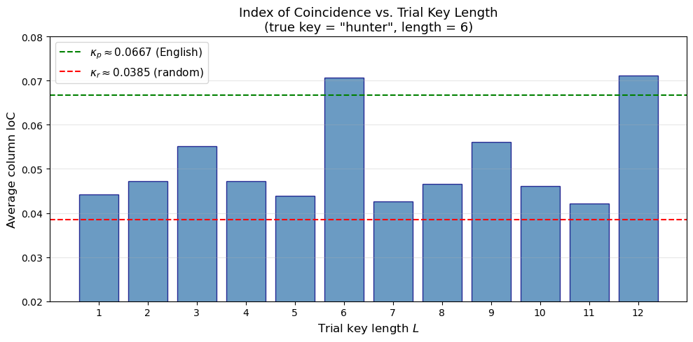
Figure saved: ioc_vs_key_length.png

Observation

The bar chart shows a clear peak at \(L = 6\) (the true key length) and also at \(L = 12\) (a multiple of 6). At \(L = 6\), the average column IoC is near \(\kappa_p \approx 0.0667\), confirming that each column is governed by a single Caesar shift. For wrong key lengths, the average column IoC hovers closer to \(\kappa_r \approx 0.0385\).

Experiment 3: Full Attack – IoC for Key Length, Chi-Squared for Key Recovery#

Having determined the key length, we recover each key letter by minimizing the chi-squared statistic between the column’s shifted frequency distribution and the expected English frequencies.

import numpy as np

# English letter frequencies
ENGLISH_FREQ = np.array([
    0.08167, 0.01492, 0.02782, 0.04253, 0.12702, 0.02228,
    0.02015, 0.06094, 0.06966, 0.00153, 0.00772, 0.04025,
    0.02406, 0.06749, 0.07507, 0.01929, 0.00095, 0.05987,
    0.06327, 0.09056, 0.02758, 0.00978, 0.02360, 0.00150,
    0.01974, 0.00074
])


def chi_squared_shift(column_text, shift, expected_freq):
    """Compute chi-squared statistic for a column after applying a shift.

    We shift the column letters back by `shift` and compare the resulting
    frequency distribution to the expected English frequencies.
    """
    cleaned = ''.join(ch.lower() for ch in column_text if ch.isalpha())
    N = len(cleaned)
    if N == 0:
        return float('inf')

    # Count letter frequencies after shifting back
    counts = np.zeros(26)
    for ch in cleaned:
        shifted_idx = (ord(ch) - ord('a') - shift) % 26
        counts[shifted_idx] += 1

    observed_freq = counts / N
    # Chi-squared statistic
    chi2 = np.sum((observed_freq - expected_freq) ** 2 / expected_freq)
    return chi2


def recover_key(ciphertext, key_length):
    """Recover the Vigenere key given the key length.

    For each column, try all 26 shifts and pick the one that minimizes
    the chi-squared statistic against English letter frequencies.
    """
    cleaned = ''.join(ch.lower() for ch in ciphertext if ch.isalpha())
    key = []

    for col_idx in range(key_length):
        # Extract column
        column = cleaned[col_idx::key_length]

        # Try all 26 shifts, pick the one with smallest chi-squared
        best_shift = 0
        best_chi2 = float('inf')
        for shift in range(26):
            chi2 = chi_squared_shift(column, shift, ENGLISH_FREQ)
            if chi2 < best_chi2:
                best_chi2 = chi2
                best_shift = shift

        key.append(chr(best_shift + ord('a')))

    return ''.join(key)


def select_best_key_length(ioc_results, threshold=0.060):
    """Select the most likely key length from IoC results.

    Among all candidate lengths whose average column IoC exceeds the
    threshold, prefer the smallest L.  Additionally, if a candidate L
    is a multiple of a smaller candidate L', prefer L' (divisor
    analysis: a doubled key gives equally high IoC).
    """
    # Collect candidates that exceed the threshold
    candidates = [L for L, ioc in sorted(ioc_results.items())
                  if ioc >= threshold]
    if not candidates:
        # Fall back to the length with the highest IoC
        return max(ioc_results, key=ioc_results.get)
    # Return the smallest candidate -- it will be the fundamental
    # period; larger candidates are almost always multiples of it.
    return candidates[0]


# Step 1: Determine key length via IoC
print("=" * 55)
print("FULL ATTACK ON VIGENERE CIPHER USING IoC")
print("=" * 55)

ioc_results = ioc_tool.estimate_key_length(ciphertext, max_key_length=12)
best_L = select_best_key_length(ioc_results)
print(f"\nStep 1: Key length estimation via IoC")
print(f"  Best candidate key length: L = {best_L}")
print(f"  Average column IoC at L={best_L}: {float(ioc_results[best_L]):.6f}")

# Step 2: Recover key via chi-squared
recovered_key = recover_key(ciphertext, best_L)
print(f"\nStep 2: Key recovery via chi-squared")
print(f"  Recovered key: '{recovered_key}'")
print(f"  True key:      '{key}'")
print(f"  Match: {'YES' if recovered_key == key else 'NO'}")

# Step 3: Decrypt
decrypted = vigenere_decrypt(ciphertext, recovered_key)
print(f"\nStep 3: Decrypted text (first 120 chars):")
print(f"  {decrypted[:120]}")

=======================================================
FULL ATTACK ON VIGENERE CIPHER USING IoC
=======================================================

Step 1: Key length estimation via IoC
  Best candidate key length: L = 6
  Average column IoC at L=6: 0.070684

Step 2: Key recovery via chi-squared
  Recovered key: 'hunter'
  True key:      'hunter'
  Match: YES

Step 3: Decrypted text (first 120 chars):
  ciphersohcipherssecretstheykeeplockedawayincodedeepanddiscreetsymbolsandnumbersjumbledandmixedamessageencodedreadytobefi

The attack pipeline

The complete Vigenère attack consists of two distinct phases:

Key length determination using the Index of Coincidence (this chapter) or the Kasiski examination (Chapter 5).
Key recovery using chi-squared frequency matching on each column. Once the key length \(L\) is known, the problem reduces to \(L\) independent Caesar ciphers.

Experiment 4: Friedman’s Direct Formula#

We test the direct estimation formula \(L \approx (\kappa_p - \kappa_r) / (\mathrm{IC}_{\text{obs}} - \kappa_r)\) on ciphertexts with various key lengths.

import numpy as np

# Friedman's direct key length estimation formula
kappa_p = ioc_tool.expected_ioc_english()
kappa_r = ioc_tool.expected_ioc_random()

print("Friedman's Direct Formula: L ~ (kappa_p - kappa_r) / (IC_obs - kappa_r)")
print(f"kappa_p = {float(kappa_p):.6f},  kappa_r = {float(kappa_r):.6f}")
print()

test_keys = ["ab", "key", "four", "magic", "hunter", "longkey",
             "vigenere", "tenletkey", "encryption"]

print(f"{'Key':>12s}  {'True L':>7s}  {'IC_obs':>8s}  {'Friedman L':>11s}  {'Column L':>9s}")
print("-" * 55)

for k in test_keys:
    ct = vigenere_encrypt(english_text, k)
    ic_obs = ioc_tool.compute_ioc(ct)

    # Friedman's formula
    if ic_obs > kappa_r:
        friedman_L = (kappa_p - kappa_r) / (ic_obs - kappa_r)
    else:
        friedman_L = float('inf')

    # Column method (prefer smallest candidate above threshold)
    ioc_est = ioc_tool.estimate_key_length(ct, max_key_length=15)
    column_L = select_best_key_length(ioc_est)

    print(f"{k:>12s}  {int(len(k)):>7d}  {float(ic_obs):>8.5f}  {float(friedman_L):>11.2f}  {int(column_L):>9d}")

Friedman's Direct Formula: L ~ (kappa_p - kappa_r) / (IC_obs - kappa_r)
kappa_p = 0.065497,  kappa_r = 0.038462

         Key   True L    IC_obs   Friedman L   Column L
-------------------------------------------------------
          ab        2   0.05532         1.60          2
         key        3   0.04700         3.16          3
        four        4   0.04587         3.65          4
       magic        5   0.04418         4.73          5
      hunter        6   0.04425         4.67          6
     longkey        7   0.04119         9.89          7
    vigenere        8   0.04625         3.47          8
   tenletkey        9   0.04475         4.30          9
  encryption       10   0.04374         5.12         10

Observation

Friedman’s direct formula gives a rough floating-point estimate of \(L\). The column-based method (Experiment 2) is more reliable in practice because it directly tests each candidate \(L\) and does not depend on a single global IoC measurement. However, the direct formula is useful for a quick initial estimate, especially when one wants to narrow the search range.

Experiment 5: Comparing Kasiski vs. IoC on the Same Ciphertext#

We implement a simplified Kasiski examination and compare its output with the IoC column method.

import numpy as np


def kasiski_examination(ciphertext, min_ngram=3, max_ngram=5):
    """Perform Kasiski examination to estimate key length.

    Finds repeated n-grams, computes distances between occurrences,
    and returns factor counts to estimate key length.
    """
    cleaned = ''.join(ch.lower() for ch in ciphertext if ch.isalpha())
    distances = []

    for n in range(min_ngram, max_ngram + 1):
        # Find all n-gram positions
        ngram_positions = {}
        for i in range(len(cleaned) - n + 1):
            ngram = cleaned[i:i + n]
            if ngram in ngram_positions:
                ngram_positions[ngram].append(i)
            else:
                ngram_positions[ngram] = [i]

        # Compute distances between repeated n-grams
        for ngram, positions in ngram_positions.items():
            if len(positions) >= 2:
                for i in range(len(positions)):
                    for j in range(i + 1, len(positions)):
                        distances.append(positions[j] - positions[i])

    if not distances:
        return {}

    # Count factors of all distances
    factor_counts = {}
    for d in distances:
        for f in range(2, min(d + 1, 21)):  # check factors up to 20
            if d % f == 0:
                factor_counts[f] = factor_counts.get(f, 0) + 1

    return factor_counts


# Compare on the same ciphertext
print("=" * 60)
print("COMPARISON: Kasiski Examination vs. Index of Coincidence")
print(f"True key: '{key}' (length {len(key)})")
print("=" * 60)

# Kasiski
print("\n--- Kasiski Examination ---")
factor_counts = kasiski_examination(ciphertext)
if factor_counts:
    sorted_factors = sorted(factor_counts.items(), key=lambda x: x[1], reverse=True)
    print(f"{'Factor':>8s}  {'Count':>6s}")
    print("-" * 18)
    for factor, count in sorted_factors[:10]:
        marker = " <--" if factor == len(key) else ""
        print(f"{int(factor):>8d}  {int(count):>6d}{marker}")
    kasiski_best = sorted_factors[0][0]
    print(f"\nKasiski best guess: L = {kasiski_best}")
else:
    print("No repeated n-grams found (text too short for Kasiski).")
    kasiski_best = None

# IoC column method
print("\n--- Index of Coincidence (Column Method) ---")
ioc_results = ioc_tool.estimate_key_length(ciphertext, max_key_length=12)
print(f"{'L':>3s}  {'Avg Col IoC':>12s}")
print("-" * 20)
for L in range(1, 13):
    marker = " <--" if ioc_results[L] > 0.060 else ""
    print(f"{int(L):>3d}  {float(ioc_results[L]):>12.6f}{marker}")
ioc_best = select_best_key_length(ioc_results)
print(f"\nIoC best guess: L = {ioc_best}")

============================================================
COMPARISON: Kasiski Examination vs. Index of Coincidence
True key: 'hunter' (length 6)
============================================================

--- Kasiski Examination ---
  Factor   Count
------------------
       2     127
       3     120
       6     120 <--
       4      59
      12      54
       9      33
      18      33
       7      17
      14      17
       8      15

Kasiski best guess: L = 2

--- Index of Coincidence (Column Method) ---
  L   Avg Col IoC
--------------------
  1      0.044249
  2      0.047276
  3      0.055169
  4      0.047285
  5      0.043817
  6      0.070684 <--
  7      0.042595
  8      0.046647
  9      0.056016
 10      0.046104
 11      0.042155
 12      0.071212 <--

IoC best guess: L = 6

../_images/94f18cd218329d9c2d48643dcde47db229e8557502e17a903d5bd0cd3f929dd7.png

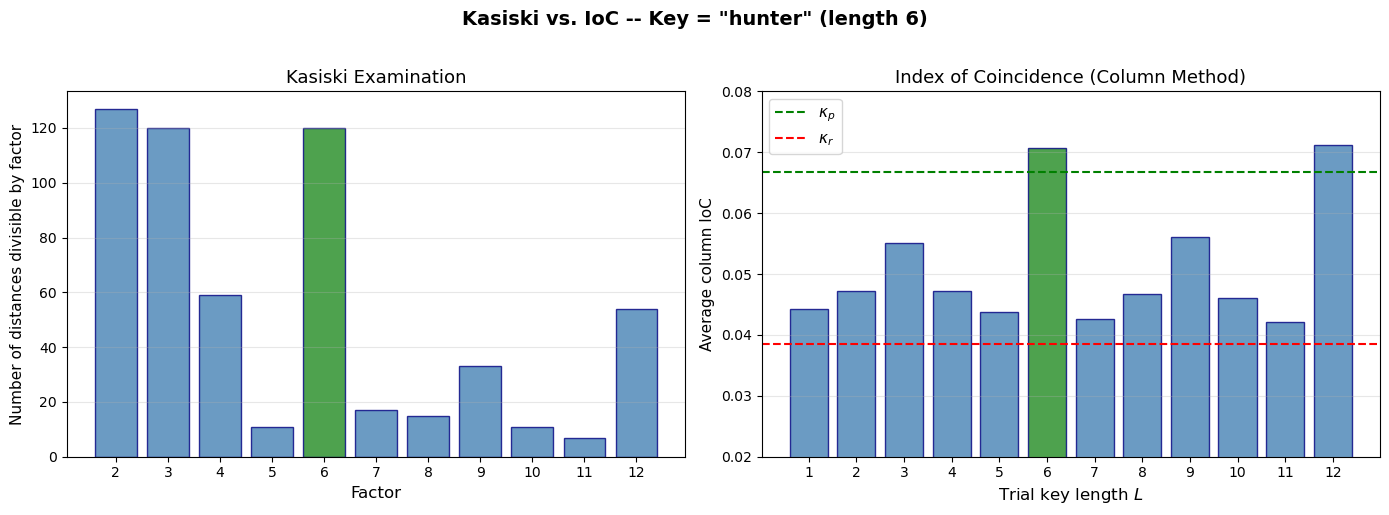
Figure saved: kasiski_vs_ioc_comparison.png

Experiment 6: IoC Convergence as Text Length Grows#

We study how the IoC of a text stabilizes as the sample size increases, for both English and random text.

../_images/5dc07cf3a8a8490d521feca4d577e627adfa7bf25d93483caa11c3c5fa3492d6.png

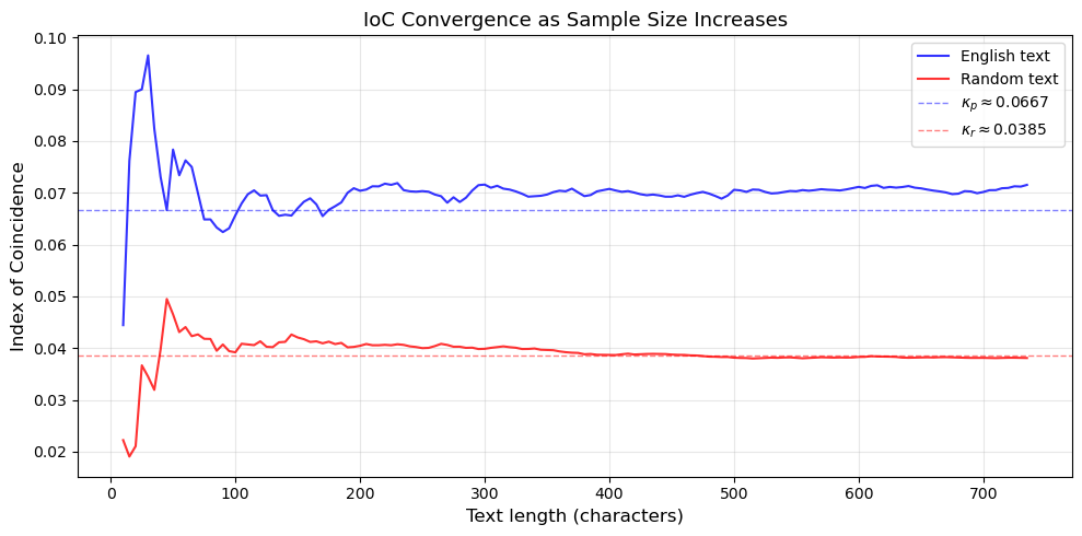
Figure saved: ioc_convergence.png

Observation

The IoC is noisy for short texts (fewer than about 50 characters) but quickly stabilizes. The English text converges toward \(\kappa_p \approx 0.0667\), while random text converges toward \(\kappa_r \approx 0.0385\). This means the IoC method becomes reliable with as few as 100-200 characters of ciphertext – far less than the Kasiski examination typically requires.

Experiment 7: Visualizing the Theoretical IC vs. Key Length#

We plot Friedman’s theoretical formula alongside empirically measured IoC values.

../_images/f81cef9cc076cf867cf9b8eee4a129dbac9701ad06848af80af0052bbfc3fa88.png

Figure saved: friedman_theoretical_vs_empirical.png

Observation

The empirical IoC values closely follow Friedman’s theoretical curve. For \(L = 1\) (Caesar cipher), the IoC is near \(\kappa_p\) because a single shift preserves the frequency distribution. As \(L\) increases, the IoC drops monotonically toward \(\kappa_r\), because the superposition of multiple shifted alphabets flattens the overall frequency distribution. The slight deviations from theory arise from the finite length of our sample text.

Experiment 8: Mutual Index of Coincidence#

We demonstrate the Mutual IoC by comparing columns of a Vigenère ciphertext that were encrypted with the same key letter versus different key letters.

Mutual Index of Coincidence between columns
Key = 'hunter' (length 6)
Key letters: ['h', 'u', 'n', 't', 'e', 'r']

     Col 0  Col 1  Col 2  Col 3  Col 4  Col 5
Col 0  0.0708 0.0473 0.0286 0.0429 0.0409 0.0454
Col 1  0.0473 0.0881 0.0391 0.0427 0.0401 0.0339
Col 2  0.0286 0.0391 0.0745 0.0281 0.0356 0.0364
Col 3  0.0429 0.0427 0.0281 0.0818 0.0487 0.0323
Col 4  0.0409 0.0401 0.0356 0.0487 0.0783 0.0433
Col 5  0.0454 0.0339 0.0364 0.0323 0.0433 0.0761

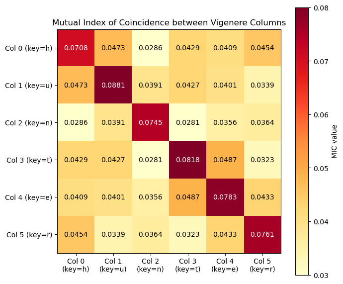
../_images/e9829e827750d0d6bcf4b99dcdd6ee37f7de9fc7568731c85cd96ac954a74fb1.png

Figure saved: mutual_ioc_heatmap.png

Observation

The diagonal entries (each column compared with itself) show the IoC of individual columns, which should be near \(\kappa_p \approx 0.0667\). The off-diagonal entries show the MIC between columns encrypted with different key letters. If two columns happen to use key letters that are close together in the alphabet (small relative shift), their MIC may be higher; otherwise it will be closer to \(\kappa_r\). The MIC can be used to determine the relative shift between two columns, which is useful for key recovery.

Exercises#

Exercise 6.1: IoC for different languages

The letter frequency distributions differ across languages. The following table gives approximate \(\kappa_p\) values for several languages:

Language	\(\kappa_p\)
English	0.0667
French	0.0778
German	0.0762
Italian	0.0738
Spanish	0.0775
Russian	0.0529

(a) Explain why Russian has a lower \(\kappa_p\) than the other languages listed. (Hint: consider the alphabet size.)

(b) Using the French frequency distribution below, compute \(\kappa_p\) for French and verify it is approximately 0.0778.

# French letter frequencies (A-Z)
french_freq = [
    0.0815, 0.0097, 0.0315, 0.0373, 0.1739, 0.0112,
    0.0097, 0.0085, 0.0731, 0.0045, 0.0002, 0.0546,
    0.0296, 0.0712, 0.0528, 0.0303, 0.0099, 0.0655,
    0.0808, 0.0707, 0.0574, 0.0132, 0.0004, 0.0045,
    0.0030, 0.0012
]

(c) How would Friedman’s key length formula change for a French-language ciphertext?

Exercise 6.2: Proving IoC invariance

Prove that the Index of Coincidence is invariant under any monoalphabetic substitution cipher. That is, if \(\sigma: \mathcal{A} \to \mathcal{A}\) is a bijection and \(y = \sigma(x_1)\sigma(x_2)\cdots\sigma(x_N)\), then \(\mathrm{IC}(y) = \mathrm{IC}(x)\).

Hint: A bijection \(\sigma\) merely permutes the frequency counts \(\{f_0, f_1, \ldots, f_{25}\}\), but the IoC formula is a symmetric function of these counts.

Exercise 6.3: Implementing Friedman’s key length formula

Write a function friedman_estimate(ciphertext) that:

Computes the observed IoC of the ciphertext.
Applies the formula \(L \approx (\kappa_p - \kappa_r) / (\mathrm{IC}_{\text{obs}} - \kappa_r)\).
Returns the nearest integer as the estimated key length.

Test your function on the ciphertext produced by encrypting the text "the quick brown fox jumps over the lazy dog" repeated 20 times with the keys "ab", "code", "secret", and "cryptanalysis". Compare the estimates with the true key lengths.

Exercise 6.4: IoC of a running-key cipher

A running-key cipher uses a key that is as long as the plaintext (typically taken from a book or other natural-language text).

(a) What is the expected IoC of ciphertext produced by a running-key cipher? (Hint: The key length \(L = N\), the text length.)

(b) Encrypt a 500-character English plaintext using a 500-character English key (from a different source). Compute the IoC and compare it to \(\kappa_r\).

(c) Explain why the IoC method alone cannot distinguish between a running-key cipher and a one-time pad with truly random key.

Exercise 6.5: Automated Vigenère attack

Write a complete function break_vigenere(ciphertext, max_key_length=20) that:

Uses the IoC column method to determine the key length.
Uses the chi-squared method to recover each key letter.
Returns the recovered key and the decrypted plaintext.

Test your function on the following ciphertext (encrypted with an unknown key of unknown length):

lxfopvefrnhr...

Generate your own test ciphertext by encrypting a paragraph from a book with a key of your choice, then verify that your function recovers the correct key.

Summary#

In this chapter we introduced the Index of Coincidence, a statistical tool invented by William F. Friedman that revolutionized the cryptanalysis of polyalphabetic ciphers.

Key concepts:

Index of Coincidence (IoC): The probability that two randomly chosen letters from a text are the same: \(\mathrm{IC}(x) = \sum f_i(f_i - 1) / N(N-1)\).
Benchmark values: English text has \(\kappa_p \approx 0.0667\); uniformly random text has \(\kappa_r = 1/26 \approx 0.0385\).
Invariance: The IoC is invariant under monoalphabetic substitution (any permutation of the alphabet).
Friedman’s Theorem: For a polyalphabetic cipher with key length \(L\), the expected IoC is \(\mathrm{IC} \approx (\kappa_p - \kappa_r)/L + \kappa_r\).
Key length estimation: The column method splits ciphertext into \(L\) columns and checks whether the average column IoC is close to \(\kappa_p\). Peaks at the correct \(L\) and its multiples.
Mutual IoC: Measures the similarity between two texts and can be used to determine relative shifts between Vigenère columns.
Comparison with Kasiski: The IoC method is more robust for shorter texts and does not require the ciphertext to contain repeated n-grams.

Together with the Kasiski examination (Chapter 5), the IoC gives the cryptanalyst a powerful toolkit for breaking the Vigenère cipher. In practice, the two methods complement each other: Kasiski gives exact divisors while the IoC gives a continuous statistical measure.

References#

Friedman, W. F. (1922). The Index of Coincidence and Its Applications in Cryptanalysis. Riverbank Publication No. 22. Department of Ciphers, Riverbank Laboratories, Geneva, Illinois. [1]
Kasiski, F. W. (1863). Die Geheimschriften und die Dechiffrir-Kunst. Berlin: E. S. Mittler und Sohn. [2]
Sinkov, A. (1966). Elementary Cryptanalysis: A Mathematical Approach. Mathematical Association of America. – Chapters 4-5 provide an accessible introduction to the IoC and Kasiski methods.
Bauer, F. L. (2007). Decrypted Secrets: Methods and Maxims of Cryptology. 4th edition, Springer. – Chapter 3 gives a thorough treatment of polyalphabetic ciphers and the IoC.
Singh, S. (1999). The Code Book: The Science of Secrecy from Ancient Egypt to Quantum Cryptography. Doubleday. [3] – Chapter 2 tells the story of Friedman and the breaking of polyalphabetic ciphers.
Kahn, D. (1996). The Codebreakers: The Comprehensive History of Secret Communication from Ancient Times to the Internet. Revised edition, Scribner. – Chapters 12-13 cover Friedman’s contributions in detail.

Chapter 6: Index of Coincidence

Contents

Chapter 6: Index of Coincidence#

6.1 History: William F. Friedman and the Statistical Revolution#

6.2 Formal Definitions#

6.2.1 The Index of Coincidence#

6.2.2 Expected IoC for English: \(\kappa_p\)#

6.2.3 Expected IoC for Random Text: \(\kappa_r\)#

6.2.4 Mutual Index of Coincidence#

6.3 Implementation#

6.4 Key Results#

6.4.1 Friedman’s Theorem#

6.4.2 Key Length Estimation#

6.4.3 Column-Based Method#

6.4.4 Comparison with Kasiski#

Experiments#

Experiment 1: IoC is Invariant Under Monoalphabetic Substitution#

Experiment 2: IoC vs. Key Length for Vigenère Ciphertext#

Experiment 3: Full Attack – IoC for Key Length, Chi-Squared for Key Recovery#

Experiment 4: Friedman’s Direct Formula#

Experiment 5: Comparing Kasiski vs. IoC on the Same Ciphertext#

Experiment 6: IoC Convergence as Text Length Grows#

Experiment 7: Visualizing the Theoretical IC vs. Key Length#

Experiment 8: Mutual Index of Coincidence#

Exercises#

Summary#

References#