Chapter 1: Introduction to Cryptanalysis

1.1 Introduction: The Eternal Arms Race

The history of cryptanalysis is as old as the history of secret writing itself. For as long as humans have sought to conceal messages, others have devoted their intellect to revealing them. The earliest known treatise on cryptanalysis is the Risalah fi Istikhraj al-Mu’amma (“Manuscript on Deciphering Cryptographic Messages”), written by the Arab polymath Abu Yusuf Ya’qub ibn Ishaq al-Kindi around 850 AD in Baghdad. Al-Kindi introduced the technique of frequency analysis – the observation that in any sufficiently long text written in a natural language, certain letters appear with predictable regularity. By comparing the frequency distribution of symbols in a ciphertext against the known distribution of the underlying language, one can peel away the veil of substitution ciphers. This single insight rendered every monoalphabetic substitution cipher insecure and inaugurated the scientific study of code-breaking.

A millennium later, the Dutch-born linguist and cryptographer Auguste Kerckhoffs (1835–1903) formulated six design principles for military ciphers in his landmark 1883 paper La Cryptographie Militaire. The second of these principles has become the cornerstone of modern cryptographic design:

“Il faut qu’il n’exige pas le secret, et qu’il puisse sans inconvénient tomber entre les mains de l’ennemi.”

(“It must not require secrecy, and it must be able to fall into the enemy’s hands without inconvenience.”)

– Auguste Kerckhoffs, La Cryptographie Militaire (1883)

Kerckhoffs recognized a profound truth: in any large-scale deployment of a cipher – across an army, a government, or an entire network – the algorithm will inevitably leak. Captured codebooks, reverse-engineered devices, disloyal insiders, or simple espionage will eventually expose the mechanism. Security must therefore reside not in the obscurity of the method, but in the secrecy of a short, easily changeable key. This insight separated the study of cryptography from the mere art of concealment and elevated it toward a principled engineering discipline.

The mathematical formalization of these ideas arrived in 1949, when Claude Elwood Shannon – working at Bell Labs – published Communication Theory of Secrecy Systems. Shannon cast cryptography in the language of information theory, defining concepts such as perfect secrecy, unicity distance, and redundancy with mathematical precision. He restated Kerckhoffs’s principle in its most succinct modern form:

“The enemy knows the system being used.”

– Claude Shannon, Communication Theory of Secrecy Systems (1949)

Shannon proved that perfect secrecy – where the ciphertext reveals absolutely no information about the plaintext – requires a key at least as long as the message itself (the one-time pad). This result established an information-theoretic lower bound that no amount of computational ingenuity can circumvent, and it set the stage for the modern distinction between information-theoretic and computational security.

Tip

Interdisciplinary thinking is essential. Cryptanalysis draws on number theory, linear algebra, statistics, combinatorics, information theory, and computer science. The most powerful attacks in history have come from unexpected angles: linguists exploiting letter frequencies, mathematicians finding algebraic weaknesses, engineers exploiting timing variations. As you study this material, cultivate breadth alongside depth.

1.2 Formal Definitions

Before we can study how to break cryptosystems, we must define precisely what a cryptosystem is.

Definition 1.1 (Cryptosystem)

A cryptosystem is a 5-tuple \((\mathcal{P}, \mathcal{C}, \mathcal{K}, \mathcal{E}, \mathcal{D})\) where:

• \(\mathcal{P}\) is a finite set called the plaintext space,

• \(\mathcal{C}\) is a finite set called the ciphertext space,

• \(\mathcal{K}\) is a finite set called the key space,

• \(\mathcal{E} = \{E_k : \mathcal{P} \to \mathcal{C} \mid k \in \mathcal{K}\}\) is a family of encryption functions,

• \(\mathcal{D} = \{D_k : \mathcal{C} \to \mathcal{P} \mid k \in \mathcal{K}\}\) is a family of decryption functions,

satisfying the correctness condition: for every key \(k \in \mathcal{K}\) and every message \(m \in \mathcal{P}\),

\[ D_k(E_k(m)) = m.\]

This definition captures the essential structure of any symmetric cipher. For public-key cryptosystems, the key space is partitioned into pairs \((k_e, k_d)\) of encryption and decryption keys, but the correctness condition remains the same.

Definition 1.2 (Kerckhoffs’s Principle)

A cryptosystem should be secure even if everything about the system – the sets \(\mathcal{P}\), \(\mathcal{C}\), \(\mathcal{K}\) and the function families \(\mathcal{E}\), \(\mathcal{D}\) – is public knowledge. The only secret is the specific key \(k \in \mathcal{K}\) in use.

Formally, for any adversary \(\mathcal{A}\) given full knowledge of \((\mathcal{P}, \mathcal{C}, \mathcal{K}, \mathcal{E}, \mathcal{D})\) but not \(k\), the advantage of \(\mathcal{A}\) should be negligible.

Kerckhoffs’s principle has a direct practical implication: open design. Algorithms that have been publicly scrutinized by the global research community for years (e.g., AES, SHA-3) inspire far more confidence than proprietary algorithms whose security rests on the hope that no one will reverse-engineer them.

Definition 1.3 (Attack Taxonomy)

Cryptanalytic attacks are classified by the information available to the adversary:

Attack Model	Abbreviation	Adversary’s Capabilities
Ciphertext-only attack	COA	Access to one or more ciphertexts \(c_1, c_2, \ldots\)
Known-plaintext attack	KPA	Access to plaintext-ciphertext pairs \((m_i, c_i)\)
Chosen-plaintext attack	CPA	Can choose plaintexts \(m_i\) and obtain \(c_i = E_k(m_i)\)
Chosen-ciphertext attack	CCA	Can choose ciphertexts \(c_i\) and obtain \(m_i = D_k(c_i)\)
Adaptive chosen-plaintext attack	ACPA	CPA where each query may depend on previous answers
Related-key attack	RKA	Can obtain encryptions under keys related to \(k\) by a known relation

These models are ordered roughly by the power given to the adversary: COA \(\subset\) KPA \(\subset\) CPA \(\subset\) ACPA, with CCA and RKA representing orthogonal extensions.

Danger

Security through obscurity is not security.

History is littered with examples of proprietary algorithms that were broken shortly after their details leaked: the CSS encryption on DVDs, the A5/1 cipher used in GSM mobile telephony, and the Crypto-1 cipher on MIFARE Classic smart cards. In each case, the designers relied on the secrecy of the algorithm rather than the strength of the key. When the algorithm was inevitably reverse-engineered, the entire system collapsed. Kerckhoffs’s principle is not merely a theoretical nicety – it is an operational imperative.

import numpy as np
import matplotlib.pyplot as plt
%matplotlib inline


class Cryptosystem:
    """
    Abstract base class for a symmetric cryptosystem.
    
    A cryptosystem is a tuple (P, C, K, E, D) where:
    - P: plaintext space
    - C: ciphertext space  
    - K: key space
    - E: encryption function E_k: P -> C
    - D: decryption function D_k: C -> P
    
    Parameters
    ----------
    alphabet : list
        The alphabet used for plaintext and ciphertext.
    name : str
        Name of the cryptosystem.
    """
    
    def __init__(self, alphabet, name="GenericCryptosystem"):
        self.alphabet = alphabet
        self.name = name
        self.char_to_idx = {c: i for i, c in enumerate(alphabet)}
        self.idx_to_char = {i: c for i, c in enumerate(alphabet)}
        self.n = len(alphabet)
    
    def encrypt(self, plaintext, key):
        """Encrypt plaintext with the given key."""
        raise NotImplementedError
    
    def decrypt(self, ciphertext, key):
        """Decrypt ciphertext with the given key."""
        raise NotImplementedError
    
    def validate_text(self, text):
        """Check that all characters are in the alphabet."""
        return all(c in self.char_to_idx for c in text)
    
    def __repr__(self):
        return f"{self.name}(alphabet_size={self.n})"


# Quick test
import string
latin = list(string.ascii_lowercase)
cs = Cryptosystem(latin, "TestSystem")
print(f"Cryptosystem: {cs}")
print(f"Alphabet size: {cs.n}")
print(f"Valid text 'hello': {cs.validate_text('hello')}")
print(f"Valid text 'Hello': {cs.validate_text('Hello')}")

Cryptosystem: TestSystem(alphabet_size=26)
Alphabet size: 26
Valid text 'hello': True
Valid text 'Hello': False

1.3 The Landscape of Cryptanalytic Attacks

Having established the formal framework, we now examine each attack model in detail. The classification matters because a cipher that is secure against ciphertext-only attacks may be completely broken under chosen-plaintext conditions. The designer’s task is to specify the threat model – which attack capabilities the adversary is assumed to possess – and then prove (or at least argue convincingly) that the cipher withstands attacks within that model.

Ciphertext-Only Attack (COA)

In a ciphertext-only attack, the adversary observes one or more ciphertexts \(c_1, c_2, \ldots, c_t\) and attempts to recover the corresponding plaintexts \(m_1, m_2, \ldots, m_t\) or, ideally, the key \(k\) itself.

Formally, the adversary is given:

\[ \{c_i = E_k(m_i) \mid i = 1, \ldots, t\}\]

and must output some information about \(m_i\) or \(k\).

This is the weakest attack model, and any cipher that is insecure even here is considered fundamentally broken. Al-Kindi’s frequency analysis is a classic COA technique: by examining the statistical distribution of symbols in the ciphertext, one can recover a monoalphabetic substitution key without ever seeing a single plaintext.

Known-Plaintext Attack (KPA)

In a known-plaintext attack, the adversary possesses a set of plaintext-ciphertext pairs encrypted under the target key:

\[ \{(m_i, c_i) \mid c_i = E_k(m_i),\; i = 1, \ldots, t\}\]

The classic example is the breaking of the Enigma cipher during World War II. British cryptanalysts at Bletchley Park exploited the fact that German military messages often began with predictable phrases (“weather report”, “nothing to report”) – so-called cribs. These known plaintext-ciphertext correspondences dramatically reduced the search space for the daily key settings.

Chosen-Plaintext Attack (CPA)

In a chosen-plaintext attack, the adversary has access to an encryption oracle: a black box that, given any plaintext \(m\), returns \(c = E_k(m)\). The adversary can strategically choose plaintexts to probe the structure of the encryption function.

Formally, the adversary can query:

\[ \mathcal{O}_E(m) = E_k(m)\]

for any \(m \in \mathcal{P}\) of their choosing.

Differential cryptanalysis, introduced by Biham and Shamir in 1990, is the prototypical CPA technique. By encrypting pairs of plaintexts with carefully chosen differences and analyzing the resulting ciphertext differences, one can extract information about the secret key. This technique was instrumental in analyzing DES and has influenced the design of every subsequent block cipher.

Chosen-Ciphertext Attack (CCA)

In a chosen-ciphertext attack, the adversary has access to a decryption oracle:

\[ \mathcal{O}_D(c) = D_k(c)\]

This model is particularly relevant for public-key cryptosystems, where an adversary might submit specially crafted ciphertexts to a decryption server and observe the responses. Bleichenbacher’s 1998 attack on RSA PKCS#1 v1.5 is a celebrated example: by observing which ciphertexts the server accepted or rejected, the attacker could progressively recover the plaintext of any RSA-encrypted message.

Adaptive Chosen-Plaintext Attack (ACPA)

The adaptive variant of CPA allows the adversary to choose each plaintext query based on the results of previous queries. This models a more realistic interactive adversary who can refine their strategy as they learn more about the cipher. In the adaptive setting, the adversary is strictly more powerful than in the non-adaptive CPA setting, because their queries can be correlated.

Related-Key Attack (RKA)

In a related-key attack, the adversary can obtain encryptions under multiple keys that are related to the target key \(k\) by a known function \(\phi\). That is, the adversary can query \(E_{\phi(k)}(m)\) for various choices of the relation \(\phi\) and plaintext \(m\).

Related-key attacks have been mounted against reduced-round versions of AES (Biryukov, Khovratovich, 2009) and have practical implications for key-schedule design in block ciphers.

Principle 1.1 (Kerckhoffs’s Principle – Formal Implication)

If the security of a cryptosystem \((\mathcal{P}, \mathcal{C}, \mathcal{K}, \mathcal{E}, \mathcal{D})\) depends on the secrecy of the encryption algorithm \(\mathcal{E}\) rather than on the secrecy of the key \(k\), then there exists a polynomial-time adversary \(\mathcal{A}\) that can break the system once \(\mathcal{E}\) is revealed.

More precisely: suppose for a system \(S\), the key \(k^*\) is a deterministic function of the algorithm description alone (or the effective key entropy is zero when the algorithm is known). Then upon learning \(\mathcal{E}\), the adversary can recover \(k^*\) in \(O(1)\) time.

Discussion

If security depends on the secrecy of the algorithm \(\mathcal{E}\) rather than on the key, then one of the following must hold:

1. The key is hardcoded into the algorithm. In this case, learning \(\mathcal{E}\) immediately reveals \(k\), and the adversary simply reads it off. The effective key space is \(|\mathcal{K}_{\text{eff}}| = 1\).

2. The key space is trivially small. If \(|\mathcal{K}|\) is polynomially bounded, an exhaustive search over all keys takes polynomial time.

3. The algorithm contains a trapdoor that is obscured only by the algorithm’s secrecy. Once the algorithm is published, the trapdoor is visible, and the adversary can exploit it directly.

In all three cases, the adversary \(\mathcal{A}\), given the full description of \(\mathcal{E}\) and a ciphertext \(c = E_k(m)\), can recover \(m\) in time polynomial in the description length of \(\mathcal{E}\).

Conversely, a system following Kerckhoffs’s principle derives its security from a key \(k\) drawn uniformly from a large key space \(\mathcal{K}\). Even with full knowledge of \(\mathcal{E}\), an adversary must search a space of size \(|\mathcal{K}|\), which (for a well-designed system) is exponential in the key length. \(\square\)

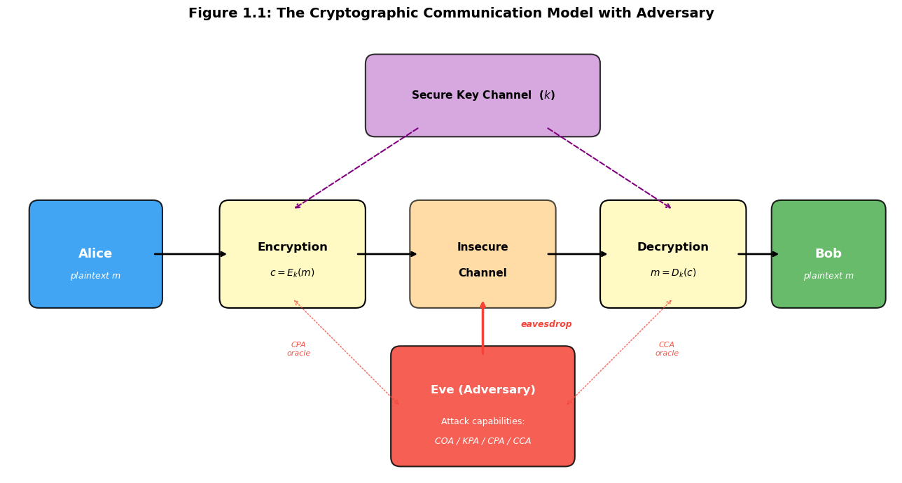
Visualization 1: The Encryption Channel and the Adversary

The following diagram illustrates the standard communication model in cryptography. Alice encrypts a message \(m\) with key \(k\) to produce ciphertext \(c\), which travels over an insecure channel to Bob, who decrypts it. Eve, the adversary, can observe the channel and, depending on her attack model, may also interact with the encryption or decryption process.

Show code cell source Hide code cell source

import numpy as np
import matplotlib.pyplot as plt
import matplotlib.patches as mpatches
%matplotlib inline

fig, ax = plt.subplots(1, 1, figsize=(14, 7))
ax.set_xlim(0, 14)
ax.set_ylim(0, 7)
ax.set_aspect('equal')
ax.axis('off')
fig.patch.set_facecolor('white')

# Color scheme
alice_color = '#2196F3'
bob_color = '#4CAF50'
eve_color = '#F44336'
box_color = '#FFF9C4'
channel_color = '#FFCC80'
key_color = '#CE93D8'

# --- Alice ---
alice_box = mpatches.FancyBboxPatch((0.5, 2.8), 1.8, 1.4, boxstyle="round,pad=0.15",
                                     facecolor=alice_color, edgecolor='black', linewidth=1.5, alpha=0.85)
ax.add_patch(alice_box)
ax.text(1.4, 3.5, 'Alice', fontsize=13, fontweight='bold', ha='center', va='center', color='white')
ax.text(1.4, 3.15, 'plaintext $m$', fontsize=9, ha='center', va='center', color='white', style='italic')

# --- Encryption box ---
enc_box = mpatches.FancyBboxPatch((3.5, 2.8), 2.0, 1.4, boxstyle="round,pad=0.15",
                                   facecolor=box_color, edgecolor='black', linewidth=1.5)
ax.add_patch(enc_box)
ax.text(4.5, 3.6, 'Encryption', fontsize=12, fontweight='bold', ha='center', va='center')
ax.text(4.5, 3.2, '$c = E_k(m)$', fontsize=10, ha='center', va='center', style='italic')

# --- Channel ---
channel_box = mpatches.FancyBboxPatch((6.5, 2.8), 2.0, 1.4, boxstyle="round,pad=0.15",
                                       facecolor=channel_color, edgecolor='black', linewidth=1.5, alpha=0.7)
ax.add_patch(channel_box)
ax.text(7.5, 3.6, 'Insecure', fontsize=11, fontweight='bold', ha='center', va='center')
ax.text(7.5, 3.2, 'Channel', fontsize=11, fontweight='bold', ha='center', va='center')

# --- Decryption box ---
dec_box = mpatches.FancyBboxPatch((9.5, 2.8), 2.0, 1.4, boxstyle="round,pad=0.15",
                                   facecolor=box_color, edgecolor='black', linewidth=1.5)
ax.add_patch(dec_box)
ax.text(10.5, 3.6, 'Decryption', fontsize=12, fontweight='bold', ha='center', va='center')
ax.text(10.5, 3.2, '$m = D_k(c)$', fontsize=10, ha='center', va='center', style='italic')

# --- Bob ---
bob_box = mpatches.FancyBboxPatch((12.2, 2.8), 1.5, 1.4, boxstyle="round,pad=0.15",
                                   facecolor=bob_color, edgecolor='black', linewidth=1.5, alpha=0.85)
ax.add_patch(bob_box)
ax.text(12.95, 3.5, 'Bob', fontsize=13, fontweight='bold', ha='center', va='center', color='white')
ax.text(12.95, 3.15, 'plaintext $m$', fontsize=9, ha='center', va='center', color='white', style='italic')

# --- Arrows between boxes ---
arrow_style = dict(arrowstyle='->', color='black', lw=2)
ax.annotate('', xy=(3.5, 3.5), xytext=(2.3, 3.5), arrowprops=arrow_style)
ax.annotate('', xy=(6.5, 3.5), xytext=(5.5, 3.5), arrowprops=arrow_style)
ax.annotate('', xy=(9.5, 3.5), xytext=(8.5, 3.5), arrowprops=arrow_style)
ax.annotate('', xy=(12.2, 3.5), xytext=(11.5, 3.5), arrowprops=arrow_style)

# --- Key distribution (top) ---
key_box = mpatches.FancyBboxPatch((5.8, 5.5), 3.4, 1.0, boxstyle="round,pad=0.15",
                                   facecolor=key_color, edgecolor='black', linewidth=1.5, alpha=0.8)
ax.add_patch(key_box)
ax.text(7.5, 6.0, 'Secure Key Channel  ($k$)', fontsize=11, fontweight='bold',
        ha='center', va='center')

ax.annotate('', xy=(4.5, 4.2), xytext=(6.5, 5.5),
            arrowprops=dict(arrowstyle='->', color='purple', lw=1.5, ls='--'))
ax.annotate('', xy=(10.5, 4.2), xytext=(8.5, 5.5),
            arrowprops=dict(arrowstyle='->', color='purple', lw=1.5, ls='--'))

# --- Eve (adversary) ---
eve_box = mpatches.FancyBboxPatch((6.2, 0.3), 2.6, 1.6, boxstyle="round,pad=0.15",
                                   facecolor=eve_color, edgecolor='black', linewidth=1.5, alpha=0.85)
ax.add_patch(eve_box)
ax.text(7.5, 1.35, 'Eve (Adversary)', fontsize=12, fontweight='bold',
        ha='center', va='center', color='white')
ax.text(7.5, 0.85, 'Attack capabilities:', fontsize=9, ha='center', va='center', color='white')
ax.text(7.5, 0.55, 'COA / KPA / CPA / CCA', fontsize=9, ha='center', va='center',
        color='white', style='italic')

# Eve's eavesdropping arrow
ax.annotate('', xy=(7.5, 2.8), xytext=(7.5, 1.9),
            arrowprops=dict(arrowstyle='->', color=eve_color, lw=2.5))
ax.text(8.1, 2.35, 'eavesdrop', fontsize=9, color=eve_color, fontweight='bold', style='italic')

# Eve's oracle access arrows (CPA/CCA)
ax.annotate('', xy=(4.5, 2.8), xytext=(6.2, 1.1),
            arrowprops=dict(arrowstyle='<->', color=eve_color, lw=1.2, ls=':', alpha=0.7))
ax.text(4.6, 1.9, 'CPA\noracle', fontsize=8, color=eve_color, alpha=0.9, ha='center', style='italic')

ax.annotate('', xy=(10.5, 2.8), xytext=(8.8, 1.1),
            arrowprops=dict(arrowstyle='<->', color=eve_color, lw=1.2, ls=':', alpha=0.7))
ax.text(10.4, 1.9, 'CCA\noracle', fontsize=8, color=eve_color, alpha=0.9, ha='center', style='italic')

ax.set_title('Figure 1.1: The Cryptographic Communication Model with Adversary',
             fontsize=14, fontweight='bold', pad=15)

plt.tight_layout()
plt.savefig('fig_1_1_crypto_model.png', dpi=150, bbox_inches='tight', facecolor='white')
plt.show()

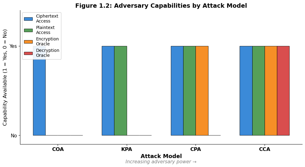
Visualization 2: Information Available to the Adversary

Different attack models grant the adversary access to different types of information. The following grouped bar chart summarizes what each attack model provides.

Show code cell source Hide code cell source

import numpy as np
import matplotlib.pyplot as plt
%matplotlib inline

# Attack models and capabilities
attack_models = ['COA', 'KPA', 'CPA', 'CCA']
capabilities = ['Ciphertext\nAccess', 'Plaintext\nAccess', 'Encryption\nOracle', 'Decryption\nOracle']

# Data: 1 = has capability, 0 = does not
# Rows: attack models (COA, KPA, CPA, CCA)
# Cols: capabilities (ciphertext, plaintext, enc oracle, dec oracle)
data = np.array([
    [1, 0, 0, 0],  # COA
    [1, 1, 0, 0],  # KPA
    [1, 1, 1, 0],  # CPA
    [1, 1, 1, 1],  # CCA
])

n_models = len(attack_models)
n_caps = len(capabilities)
x = np.arange(n_models)
width = 0.18

colors = ['#1976D2', '#388E3C', '#F57C00', '#D32F2F']

fig, ax = plt.subplots(figsize=(10, 5.5))

for i in range(n_caps):
    offset = (i - n_caps / 2 + 0.5) * width
    bars = ax.bar(x + offset, data[:, i], width, label=capabilities[i],
                  color=colors[i], edgecolor='black', linewidth=0.8, alpha=0.85)

ax.set_xlabel('Attack Model', fontsize=13, fontweight='bold')
ax.set_ylabel('Capability Available (1 = Yes, 0 = No)', fontsize=12)
ax.set_title('Figure 1.2: Adversary Capabilities by Attack Model', fontsize=14, fontweight='bold')
ax.set_xticks(x)
ax.set_xticklabels(attack_models, fontsize=12, fontweight='bold')
ax.set_yticks([0, 1])
ax.set_yticklabels(['No', 'Yes'], fontsize=11)
ax.set_ylim(-0.1, 1.4)
ax.legend(loc='upper left', fontsize=10, framealpha=0.9)
ax.spines['top'].set_visible(False)
ax.spines['right'].set_visible(False)

# Add annotation
ax.annotate('Increasing adversary power \u2192', xy=(0.5, -0.14), xycoords='axes fraction',
            fontsize=11, ha='center', style='italic', color='gray')

plt.tight_layout()
plt.savefig('fig_1_2_attack_capabilities.png', dpi=150, bbox_inches='tight', facecolor='white')
plt.show()

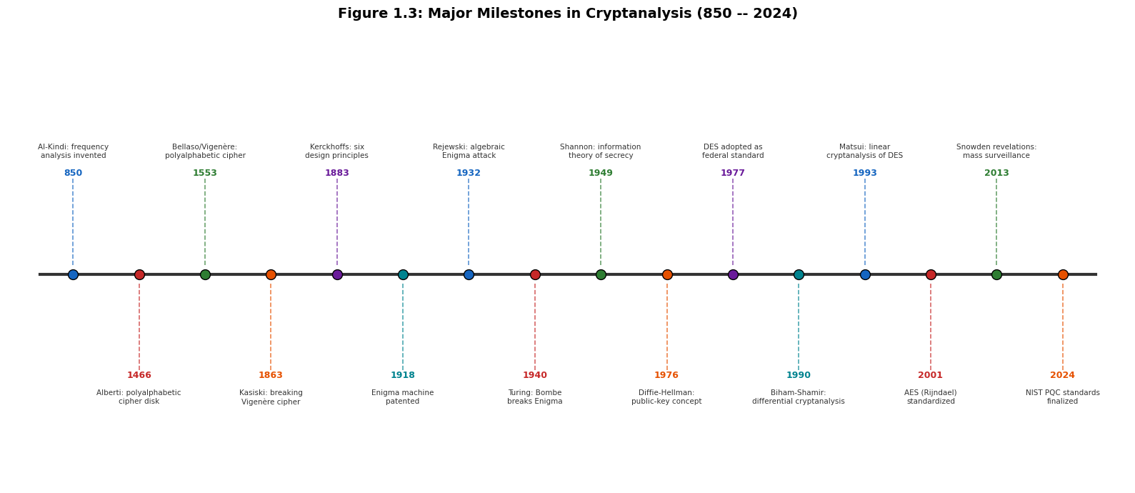
Visualization 3: A Timeline of Cryptanalytic Milestones

Cryptanalysis has a rich history spanning over a millennium. The following timeline highlights key milestones, from Al-Kindi’s invention of frequency analysis to the NIST Post-Quantum Cryptography standardization.

Show code cell source Hide code cell source

import numpy as np
import matplotlib.pyplot as plt
%matplotlib inline

# Milestones: (year, label)
milestones = [
    (850,  "Al-Kindi: frequency\nanalysis invented"),
    (1466, "Alberti: polyalphabetic\ncipher disk"),
    (1553, "Bellaso/Vigen\u00e8re:\npolyalphabetic cipher"),
    (1863, "Kasiski: breaking\nVigen\u00e8re cipher"),
    (1883, "Kerckhoffs: six\ndesign principles"),
    (1918, "Enigma machine\npatented"),
    (1932, "Rejewski: algebraic\nEnigma attack"),
    (1940, "Turing: Bombe\nbreaks Enigma"),
    (1949, "Shannon: information\ntheory of secrecy"),
    (1976, "Diffie-Hellman:\npublic-key concept"),
    (1977, "DES adopted as\nfederal standard"),
    (1990, "Biham-Shamir:\ndifferential cryptanalysis"),
    (1993, "Matsui: linear\ncryptanalysis of DES"),
    (2001, "AES (Rijndael)\nstandardized"),
    (2013, "Snowden revelations:\nmass surveillance"),
    (2024, "NIST PQC standards\nfinalized"),
]

years = [m[0] for m in milestones]
labels = [m[1] for m in milestones]

fig, ax = plt.subplots(figsize=(16, 7))

# Normalize positions along x-axis
y_base = 3.5
x_positions = np.linspace(0.5, 15.5, len(milestones))

# Draw the horizontal timeline
ax.plot([0, 16], [y_base, y_base], color='#333333', lw=3, zorder=1)

# Alternate label positions above and below
colors_cycle = ['#1565C0', '#C62828', '#2E7D32', '#E65100', '#6A1B9A', '#00838F']

for i, (xp, year, label) in enumerate(zip(x_positions, years, labels)):
    color = colors_cycle[i % len(colors_cycle)]
    
    # Alternate above/below
    if i % 2 == 0:
        y_text = y_base + 1.6
        va = 'bottom'
        y_dot_offset = 0.15
    else:
        y_text = y_base - 1.6
        va = 'top'
        y_dot_offset = -0.15
    
    # Dot on timeline
    ax.plot(xp, y_base, 'o', color=color, markersize=10, zorder=3,
            markeredgecolor='black', markeredgewidth=1)
    
    # Vertical connector
    ax.plot([xp, xp], [y_base + y_dot_offset, y_text], color=color, lw=1.2,
            ls='--', alpha=0.7, zorder=2)
    
    # Year label
    ax.text(xp, y_text, f"{year}", fontsize=9, fontweight='bold', ha='center',
            va=va, color=color)
    
    # Description
    if i % 2 == 0:
        ax.text(xp, y_text + 0.3, label, fontsize=7.5, ha='center', va='bottom',
                color='#333333', linespacing=1.3)
    else:
        ax.text(xp, y_text - 0.3, label, fontsize=7.5, ha='center', va='top',
                color='#333333', linespacing=1.3)

ax.set_xlim(-0.5, 16.5)
ax.set_ylim(0, 7.5)
ax.axis('off')
ax.set_title('Figure 1.3: Major Milestones in Cryptanalysis (850 -- 2024)',
             fontsize=14, fontweight='bold', pad=15)

plt.tight_layout()
plt.savefig('fig_1_3_cryptanalysis_timeline.png', dpi=150, bbox_inches='tight', facecolor='white')
plt.show()

Keyspace Analysis

A fundamental question in cryptanalysis is: how large is the key space? The keyspace size determines the upper bound on the effort required for a brute-force attack. Below, we compute and visualize the keyspace sizes for several classical ciphers.

Show code cell source Hide code cell source

import numpy as np
import matplotlib.pyplot as plt
from math import factorial, log2
%matplotlib inline

# Keyspace sizes for various classical ciphers (26-letter alphabet)
ciphers = {
    'Caesar cipher': 26,
    'Affine cipher': 12 * 26,  # 12 valid 'a' values * 26 'b' values
    'Vigenere (key len 5)': 26**5,
    'Vigenere (key len 10)': 26**10,
    'Simple substitution': factorial(26),
    'Hill cipher (2x2)': 26**4,  # 456,976 (counting all 2x2 matrices over Z_26; the number of *invertible* matrices, which form valid keys, is smaller -- see Chapter 7)
    'Enigma (daily settings)': 158_962_555_217_826_360_000,  # approximate
    'DES': 2**56,
    'AES-128': 2**128,
    'AES-256': 2**256,
}

print("Cipher Keyspace Sizes")
print("=" * 65)
for cipher, size in ciphers.items():
    bits = log2(size)
    print(f"{cipher:<28s}  |K| = {size:>50,}  ({float(bits):>8.1f} bits)")

# Bar chart of log2(keyspace)
names = list(ciphers.keys())
log_sizes = [log2(v) for v in ciphers.values()]

fig, ax = plt.subplots(figsize=(12, 6))

colors = plt.cm.viridis(np.linspace(0.15, 0.85, len(names)))
bars = ax.barh(range(len(names)), log_sizes, color=colors, edgecolor='black', linewidth=0.7)

ax.set_yticks(range(len(names)))
ax.set_yticklabels(names, fontsize=10)
ax.set_xlabel('Key Space Size (bits = $\\log_2 |\\mathcal{K}|$)', fontsize=12, fontweight='bold')
ax.set_title('Figure 1.4: Keyspace Sizes of Classical and Modern Ciphers', fontsize=13, fontweight='bold')
ax.invert_yaxis()
ax.spines['top'].set_visible(False)
ax.spines['right'].set_visible(False)

# Add bit-count labels
for i, (bar, bits) in enumerate(zip(bars, log_sizes)):
    ax.text(bits + 1, i, f'{float(bits):.1f} bits', va='center', fontsize=9, fontweight='bold')

# Annotate brute-force thresholds
ax.axvline(x=80, color='red', linestyle='--', alpha=0.6, linewidth=1.5)
ax.text(81, len(names) - 0.5, '80-bit security\nthreshold', fontsize=8,
        color='red', va='top', style='italic')

plt.tight_layout()
plt.savefig('fig_1_4_keyspace_sizes.png', dpi=150, bbox_inches='tight', facecolor='white')
plt.show()

1.4 Exercises

The following exercises reinforce the concepts introduced in this chapter. They range from straightforward calculations to a challenge-level proof.

---

Exercise 1.1 (Keyspace Enumeration). Compute the exact keyspace size \(|\mathcal{K}|\) for each of the following ciphers over a 26-letter English alphabet:

(a) The Caesar cipher.
(b) The affine cipher \(E_{a,b}(x) = ax + b \pmod{26}\), where \(\gcd(a, 26) = 1\).
(c) The Vigen`ere cipher with keyword length \(\ell\).
(d) The simple monoalphabetic substitution cipher.
(e) The Hill cipher with an \(n \times n\) key matrix over \(\mathbb{Z}_{26}\).

Express your answers both as exact numbers and in bits (\(\log_2 |\mathcal{K}|\)).

Hint

For (b), count the number of integers \(a \in \{0, 1, \ldots, 25\}\) coprime to 26 using Euler’s totient function: \(\phi(26) = \phi(2) \cdot \phi(13) = 1 \cdot 12 = 12\).

For (e), you need to count the number of invertible \(n \times n\) matrices over \(\mathbb{Z}_{26}\). This is related to \(|GL(n, \mathbb{Z}_2)| \cdot |GL(n, \mathbb{Z}_{13})|\) by the Chinese Remainder Theorem.

---

Exercise 1.2 (Classifying Historical Cipher Breaks). For each of the following historical cipher breaks, identify the primary attack model (COA, KPA, CPA, CCA, ACPA, or RKA) that was used. Justify your classification in one or two sentences.

(a) Al-Kindi’s frequency analysis against monoalphabetic substitution.
(b) Marian Rejewski’s algebraic attack on the Enigma machine (1932).
(c) Alan Turing’s Bombe attack on Enigma (1939–1940).
(d) Biham and Shamir’s differential cryptanalysis of DES (1990).
(e) Bleichenbacher’s attack on RSA PKCS#1 v1.5 (1998).
(f) Biryukov and Khovratovich’s attack on full AES-256 (2009).

Hint

Think about what information each attacker had access to. Al-Kindi only analyzed ciphertext. Turing exploited known plaintext (cribs). Biham and Shamir chose specific plaintext pairs. Bleichenbacher submitted chosen ciphertexts to a decryption oracle. Biryukov and Khovratovich exploited relationships between keys.

---

Exercise 1.3 (Kerckhoffs vs. Shannon – Comparative Essay). Write a short essay (approximately 300–500 words) comparing Kerckhoffs’s principle (1883) with Shannon’s maxim (1949). Address the following points:

(a) What is the historical context of each statement?
(b) Are they logically equivalent, or does one imply the other?
(c) How does each principle apply to modern open-source cryptographic software?
(d) Give an example of a system that violates both principles and explain the consequences.

Hint

Kerckhoffs was writing for a military audience concerned with operational security. Shannon was formalizing information-theoretic notions. Shannon’s maxim can be viewed as a consequence of Kerckhoffs’s principle combined with the assumption that algorithms will eventually be reverse-engineered. Consider the CSS encryption scheme on DVDs as a case study for part (d).

---

Exercise 1.4 (Brute-Force Attack Implementation). Implement a Python function brute_force_attack(ciphertext, cryptosystem, scoring_function) that:

(a) Iterates over every key \(k \in \mathcal{K}\).
(b) Decrypts the ciphertext with each key to obtain a candidate plaintext.
(c) Scores each candidate using the provided scoring_function.
(d) Returns the key and plaintext with the highest score.

Test your function on a Caesar cipher with a simple frequency-based scoring function. Encrypt a short English sentence, then recover it.

Hint

For the scoring function, use the sum of squared differences between the observed letter frequencies and the expected English letter frequencies. A lower score indicates a better match. The expected frequencies (approximate) are:

english_freq = {
    'a': 0.082, 'b': 0.015, 'c': 0.028, 'd': 0.043, 'e': 0.127,
    'f': 0.022, 'g': 0.020, 'h': 0.061, 'i': 0.070, 'j': 0.002,
    'k': 0.008, 'l': 0.040, 'm': 0.024, 'n': 0.067, 'o': 0.075,
    'p': 0.019, 'q': 0.001, 'r': 0.060, 's': 0.063, 't': 0.091,
    'u': 0.028, 'v': 0.010, 'w': 0.023, 'x': 0.002, 'y': 0.020,
    'z': 0.001
}

---

**Exercise 1.5 (Challenge: Perfect Secrecy and Keyspace Size).**
Prove the following theorem:

> **Theorem.** If a cryptosystem $(\mathcal{P}, \mathcal{C}, \mathcal{K}, \mathcal{E}, \mathcal{D})$ provides **perfect secrecy** (i.e., $\Pr[M = m \mid C = c] = \Pr[M = m]$ for all $m \in \mathcal{P}$ and $c \in \mathcal{C}$), then $|\mathcal{K}| \geq |\mathcal{P}|$.

This is one direction of Shannon's theorem characterizing perfect secrecy. It implies that the one-time pad, which uses keys as long as the messages, achieves perfect secrecy with the minimum possible key space.

```{admonition} Hint
:class: dropdown

Proceed by contradiction. Assume $|\mathcal{K}| < |\mathcal{P}|$.

1. Fix a ciphertext $c \in \mathcal{C}$ that occurs with positive probability.
2. Consider the set $\mathcal{P}(c) = \{D_k(c) \mid k \in \mathcal{K}\}$ of all possible plaintexts that could produce $c$.
3. Since $|\mathcal{P}(c)| \leq |\mathcal{K}| < |\mathcal{P}|$, there exists some $m^* \in \mathcal{P}$ with $m^* \notin \mathcal{P}(c)$.
4. Then $\Pr[M = m^* \mid C = c] = 0$, but $\Pr[M = m^*] > 0$ (assuming a uniform prior over $\mathcal{P}$).
5. This contradicts perfect secrecy.

1.5 Summary and Key Takeaways

This chapter has established the conceptual and formal foundations for the study of cryptanalysis. Here are the key takeaways:

• Cryptanalysis is as old as cryptography itself. From Al-Kindi’s frequency analysis (ca. 850 AD) to modern differential and algebraic attacks, every advance in cipher design has been met by a corresponding advance in code-breaking. This arms race is the engine that drives the field forward.

• Kerckhoffs’s principle is non-negotiable. A cryptosystem must derive its security from the key alone, not from the secrecy of the algorithm. This principle, formalized by Shannon as “the enemy knows the system,” is the bedrock of modern cryptographic design and the reason why open, publicly scrutinized standards (AES, SHA-3, CRYSTALS-Kyber) are vastly preferred over proprietary, secret algorithms.

• The attack model determines the security guarantee. A cipher that resists ciphertext-only attacks may crumble under chosen-plaintext conditions. When evaluating or designing a cryptosystem, one must specify the precise threat model – COA, KPA, CPA, CCA, ACPA, or RKA – and demonstrate security within that model.

• Keyspace size is necessary but not sufficient for security. A large key space (e.g., \(2^{256}\) for AES-256) prevents brute-force attacks, but many ciphers with enormous key spaces have been broken through structural weaknesses. The simple substitution cipher has a key space of \(26! \approx 2^{88}\) – far beyond brute-force – yet it falls trivially to frequency analysis.

Tip

Looking ahead. In Chapters 2–3, we will dive into the first major cryptanalytic technique in history: frequency analysis. We will formalize the statistical foundations behind Al-Kindi’s method, implement it in Python, and use it to break monoalphabetic substitution ciphers. This will set the stage for the polyalphabetic ciphers (Vigen`ere) studied in Chapters 5–6 and the machine ciphers (Enigma) in Chapters 10–12.

1.6 References

1. Al-Kindi, Risalah fi Istikhraj al-Mu’amma (“Manuscript on Deciphering Cryptographic Messages”), ca. 850 AD.
   The earliest known work on cryptanalysis. Al-Kindi introduced frequency analysis and demonstrated its application to breaking monoalphabetic substitution ciphers. An English translation and commentary can be found in: Ibrahim A. Al-Kadi, “The Origins of Cryptology: The Arab Contributions,” Cryptologia, 16(2), 1992.

2. Auguste Kerckhoffs, “La Cryptographie Militaire,” Journal des Sciences Militaires, vol. IX, pp. 5–38 (January 1883) and pp. 161–191 (February 1883).
   The foundational paper in which Kerckhoffs formulated his six principles for military cipher design. The second principle – that a cipher must not require secrecy and must be able to fall into enemy hands without inconvenience – has become the single most important design principle in modern cryptography.

3. Claude E. Shannon, “Communication Theory of Secrecy Systems,” Bell System Technical Journal, 28(4), pp. 656–715, 1949.
   Shannon’s seminal paper that established the information-theoretic foundations of cryptography. He formalized perfect secrecy, proved that the one-time pad is the unique cipher achieving it with minimum key size, and introduced the concept of unicity distance. This paper transformed cryptography from an art into a mathematical science.

4. Douglas R. Stinson and Maura B. Paterson, Cryptography: Theory and Practice, 4th edition, CRC Press, 2018.
   A comprehensive and mathematically rigorous textbook covering both classical and modern cryptography. Chapters 1–2 provide an excellent treatment of the formal definitions, attack models, and classical ciphers discussed in this chapter.

5. Simon Singh, The Code Book: The Science of Secrecy from Ancient Egypt to Quantum Cryptography, Anchor Books, 2000.
   An accessible and engaging popular account of the history of cryptography and cryptanalysis. Particularly recommended for historical context on Al-Kindi, the Enigma, and the development of public-key cryptography. Not a technical reference, but invaluable for building intuition and motivation.