Chapter 19 — Foundations of Differential Cryptanalysis

Chapter 19 — Foundations of Differential Cryptanalysis#

“We describe a new method for attacking DES and show that DES with a reduced number of rounds is breakable in a chosen plaintext attack.” — Eli Biham & Adi Shamir, Differential Cryptanalysis of DES-like Cryptosystems, 1991

In this chapter we develop the mathematical foundations of differential cryptanalysis, the first general-purpose attack capable of breaking DES with fewer operations than exhaustive key search. We formalize the concepts of input differences, output differences, and the difference distribution table (DDT), implement a DifferentialAnalyzer class to compute these quantities, and experimentally compare the differential properties of different S-box designs.

19.1 Historical Context#

In 1990, Eli Biham and Adi Shamir of the Weizmann Institute of Science announced a revolutionary new technique for attacking block ciphers. Their method, which they called differential cryptanalysis, was published in full in 1991. It was the first publicly known attack on the full 16-round DES that was theoretically faster than brute force (though just barely: \(2^{47}\) chosen plaintexts).

The core idea is deceptively simple: instead of analyzing the absolute values of plaintexts and ciphertexts, study how differences between pairs of plaintexts propagate through the cipher to produce differences in the corresponding ciphertexts. If certain difference patterns propagate with probability significantly higher than the ideal \(1/2^n\), the attacker can exploit this bias to recover key bits.

Year	Event
1977	DES published as FIPS 46; NSA-modified S-boxes
1990	Biham & Shamir announce differential cryptanalysis
1991	Full paper published in Journal of Cryptology
1993	Matsui announces linear cryptanalysis (complementary technique)
1994	Coppersmith reveals NSA knew about differential cryptanalysis since 1974

The most remarkable footnote to this story came in 1994, when IBM’s Don Coppersmith — one of the original DES designers — publicly confirmed that the NSA was aware of differential cryptanalysis (or a closely related technique) as early as 1974, three years before DES was published. The DES S-boxes were specifically designed to resist this attack. The design criteria, classified for nearly two decades, included:

No S-box output bit should be too close to a linear function of the input bits.
For any nonzero input difference \(\Delta X\), the set of possible output differences \(\Delta Y\) should be as uniformly distributed as possible.
The maximum entry in any S-box’s difference distribution table should be minimized.

Tip

Differential cryptanalysis is a chosen-plaintext attack: the attacker must be able to choose plaintext pairs with a specific XOR difference and observe the resulting ciphertext pairs. This is a stronger assumption than a known-plaintext attack (which linear cryptanalysis can achieve), but the technique is more powerful and has become a standard tool in the cryptanalyst’s toolkit.

19.2 Formal Definitions#

Definition 19.1 — Input and Output Differences

Let \(S: \{0,1\}^n \to \{0,1\}^m\) be a vectorial Boolean function (e.g., an S-box). Given two inputs \(X, X' \in \{0,1\}^n\), define:

The input difference: \(\Delta X = X \oplus X'\)
The output difference: \(\Delta Y = S(X) \oplus S(X')\)

The pair \((\Delta X, \Delta Y)\) is called a differential of \(S\).

The XOR operation is the natural choice for measuring differences in ciphers that use XOR-based key mixing, because the key cancels out (see Theorem 19.1).

Definition 19.2 — Difference Distribution Table (DDT)

The difference distribution table of an S-box \(S: \{0,1\}^n \to \{0,1\}^m\) is a \(2^n \times 2^m\) table where entry \((\Delta X, \Delta Y)\) counts the number of inputs \(X\) such that the ordered pair \((X,\; X \oplus \Delta X)\) produces output difference \(\Delta Y\):

\[ \text{DDT}[\Delta X][\Delta Y] = \#\{X \in \{0,1\}^n : S(X) \oplus S(X \oplus \Delta X) = \Delta Y\}\]

Note that the count iterates over all \(2^n\) individual values of \(X\). For each \(X\) that satisfies the condition, its partner \(X' = X \oplus \Delta X\) also satisfies it (see Property 4 below), so all non-trivial DDT entries are even.

Definition 19.3 — Differential Probability

The differential probability of a differential \((\Delta X \to \Delta Y)\) through an S-box \(S: \{0,1\}^n \to \{0,1\}^m\) is:

\[ \text{dp}(\Delta X \to \Delta Y) = \frac{\#\{X \in \{0,1\}^n : S(X) \oplus S(X \oplus \Delta X) = \Delta Y\}}{2^n} = \frac{\text{DDT}[\Delta X][\Delta Y]}{2^n}\]

For a random function, we expect \(\text{dp} \approx 1/2^m\). An S-box is considered differentially strong if its maximum dp (over all nonzero \(\Delta X\)) is close to this ideal bound.

Theorem 19.1 — Key Cancellation Property

Let \(F_K(X) = S(X \oplus K)\) where \(K\) is a fixed but unknown key and \(S\) is an S-box. Then the input difference is independent of the key:

\[ F_K(X) \oplus F_K(X') = S(X \oplus K) \oplus S(X' \oplus K)\]

Setting \(\tilde{X} = X \oplus K\) and \(\tilde{X}' = X' \oplus K\), we have:

\[ \tilde{X} \oplus \tilde{X}' = (X \oplus K) \oplus (X' \oplus K) = X \oplus X' = \Delta X\]

The key \(K\) cancels completely. This means that differential probabilities computed for the unkeyed S-box apply exactly to the keyed version.

Proof

The cancellation follows directly from XOR properties. Let \(A = X \oplus K\) and \(B = X' \oplus K\). Then:

\[ A \oplus B = (X \oplus K) \oplus (X' \oplus K) = X \oplus X' \oplus K \oplus K = X \oplus X'\]

since \(K \oplus K = 0\) (XOR self-cancellation). Therefore:

\[ \Delta Y = S(A) \oplus S(B) = S(X \oplus K) \oplus S(X' \oplus K)\]

depends only on \(\Delta X = X \oplus X'\) and the S-box \(S\), not on \(K\). \(\square\)

Properties of the DDT

For an S-box \(S: \{0,1\}^n \to \{0,1\}^n\) (bijective), the DDT has the following structural properties:

Row sums: Every row sums to \(2^n\) (each input \(X\) produces exactly one output difference for a given \(\Delta X\)).
First row: \(\text{DDT}[0][0] = 2^n\) and \(\text{DDT}[0][\Delta Y] = 0\) for \(\Delta Y \neq 0\) (zero input difference always gives zero output difference).
First column: \(\text{DDT}[\Delta X][0]\) counts fixed points of the mapping \(X \mapsto S(X) \oplus S(X \oplus \Delta X)\). For a bijection, this is related to the structure of the S-box.
Even entries: All DDT entries are even. This is because if \(X\) is counted (i.e., \(S(X) \oplus S(X \oplus \Delta X) = \Delta Y\)), then \(X' = X \oplus \Delta X\) is also counted, since \(S(X') \oplus S(X' \oplus \Delta X) = S(X \oplus \Delta X) \oplus S(X) = \Delta Y\). For \(\Delta X \neq 0\) we have \(X \neq X'\), so the solutions always come in distinct pairs.
Column sums (for bijective S-boxes): Every column also sums to \(2^n\).

19.3 Implementation#

We implement the DifferentialAnalyzer class that computes the DDT, extracts differential probabilities, and identifies the best differentials. We use the Heys tutorial S-box as our primary example — this is the 4-bit S-box from Heys’ widely-cited 2002 tutorial on linear and differential cryptanalysis.

import numpy as np


class DifferentialAnalyzer:
    """
    Differential cryptanalysis toolkit for S-boxes.

    Computes the difference distribution table (DDT), differential
    probabilities, and identifies the strongest differentials.

    Parameters
    ----------
    sbox : array-like
        Lookup table defining the S-box S: {0,...,2^n-1} -> {0,...,2^m-1}.
        Length must be a power of 2.
    """

    def __init__(self, sbox):
        self.sbox = np.array(sbox, dtype=int)
        self.n_inputs = len(self.sbox)
        self.input_bits = int(np.log2(self.n_inputs))
        self.output_bits = int(np.log2(max(self.sbox) + 1))
        self.n_outputs = 2 ** self.output_bits
        self._ddt = None

    def compute_ddt(self):
        """
        Compute the full difference distribution table.

        Returns
        -------
        ddt : ndarray of shape (2^n, 2^m)
            DDT[delta_in][delta_out] = count of inputs x such that
            S(x) XOR S(x XOR delta_in) = delta_out.
        """
        n_in = self.n_inputs
        n_out = self.n_outputs
        ddt = np.zeros((n_in, n_out), dtype=int)

        for delta_in in range(n_in):
            for x in range(n_in):
                x_prime = x ^ delta_in
                delta_out = int(self.sbox[x] ^ self.sbox[x_prime])
                ddt[delta_in, delta_out] += 1

        self._ddt = ddt
        return ddt

    @property
    def ddt(self):
        """Lazily compute and cache the DDT."""
        if self._ddt is None:
            self.compute_ddt()
        return self._ddt

    def differential_probability(self, delta_in, delta_out):
        """
        Look up the differential probability dp(delta_in -> delta_out).

        Returns
        -------
        float
            The probability DDT[delta_in][delta_out] / 2^n.
        """
        return self.ddt[delta_in, delta_out] / self.n_inputs

    def best_differentials(self, n=10):
        """
        Return the top-n highest-probability differentials (excluding
        the trivial differential 0 -> 0).

        Returns
        -------
        list of tuples (delta_in, delta_out, count, probability)
        """
        ddt = self.ddt.copy()
        # Exclude trivial differential (0 -> 0)
        ddt[0, 0] = 0

        # Flatten and get top-n indices
        flat_indices = np.argsort(ddt.ravel())[::-1][:n]
        results = []
        for idx in flat_indices:
            di = idx // self.n_outputs
            do = idx % self.n_outputs
            count = self.ddt[di, do]
            if count == 0:
                break
            prob = count / self.n_inputs
            results.append((di, do, count, prob))

        return results

    def max_differential_probability(self):
        """
        Return the maximum differential probability (excluding 0->0).
        """
        ddt = self.ddt.copy()
        ddt[0, 0] = 0
        max_count = np.max(ddt)
        return max_count / self.n_inputs

    def differential_uniformity(self):
        """
        Return the differential uniformity (max DDT entry, excluding 0->0).
        """
        ddt = self.ddt.copy()
        ddt[0, 0] = 0
        return int(np.max(ddt))


# --- Heys tutorial S-box ---
HEYS_SBOX = [0xE, 0x4, 0xD, 0x1, 0x2, 0xF, 0xB, 0x8,
             0x3, 0xA, 0x6, 0xC, 0x5, 0x9, 0x0, 0x7]

analyzer = DifferentialAnalyzer(HEYS_SBOX)
ddt = analyzer.compute_ddt()

print('Heys S-box:', [hex(x) for x in HEYS_SBOX])
print(f'Input bits: {analyzer.input_bits}, Output bits: {analyzer.output_bits}')
print(f'DDT shape: {ddt.shape}')
print(f'Differential uniformity: {analyzer.differential_uniformity()}')
print(f'Max dp (excl. 0->0): {float(analyzer.max_differential_probability()):.4f}')
print()
print('DifferentialAnalyzer class loaded successfully.')

Heys S-box: ['0xe', '0x4', '0xd', '0x1', '0x2', '0xf', '0xb', '0x8', '0x3', '0xa', '0x6', '0xc', '0x5', '0x9', '0x0', '0x7']
Input bits: 4, Output bits: 4
DDT shape: (16, 16)
Differential uniformity: 8
Max dp (excl. 0->0): 0.5000

DifferentialAnalyzer class loaded successfully.

import numpy as np

# Display the complete 16x16 DDT
HEYS_SBOX = [0xE, 0x4, 0xD, 0x1, 0x2, 0xF, 0xB, 0x8,
             0x3, 0xA, 0x6, 0xC, 0x5, 0x9, 0x0, 0x7]

analyzer = DifferentialAnalyzer(HEYS_SBOX)
ddt = analyzer.ddt

# Print as formatted table
header = '     ' + ''.join(f'{j:>4X}' for j in range(16))
print('Difference Distribution Table (Heys S-box)')
print('Rows = input diff (Delta_X), Cols = output diff (Delta_Y)')
print()
print(header)
print('     ' + '-' * 64)
for i in range(16):
    row = f'{i:>3X} |' + ''.join(f'{int(ddt[i,j]):>4d}' for j in range(16))
    print(row)

# Verify structural properties
print(f'\nRow sums: {np.unique(ddt.sum(axis=1))}  (expect all {analyzer.n_inputs})')
print(f'Col sums: {np.unique(ddt.sum(axis=0))}  (expect all {analyzer.n_inputs})')
print(f'All entries even: {np.all(ddt % 2 == 0)}')
print(f'DDT[0][0] = {ddt[0,0]}  (expect {analyzer.n_inputs})')
print(f'DDT[0][1:] all zero: {np.all(ddt[0, 1:] == 0)}')

Difference Distribution Table (Heys S-box)
Rows = input diff (Delta_X), Cols = output diff (Delta_Y)

        0   1   2   3   4   5   6   7   8   9   A   B   C   D   E   F
     ----------------------------------------------------------------
  0 |  16   0   0   0   0   0   0   0   0   0   0   0   0   0   0   0
  1 |   0   0   0   2   0   0   0   2   0   2   4   0   4   2   0   0
  2 |   0   0   0   2   0   6   2   2   0   2   0   0   0   0   2   0
  3 |   0   0   2   0   2   0   0   0   0   4   2   0   2   0   0   4
  4 |   0   0   0   2   0   0   6   0   0   2   0   4   2   0   0   0
  5 |   0   4   0   0   0   2   2   0   0   0   4   0   2   0   0   2
  6 |   0   0   0   4   0   4   0   0   0   0   0   0   2   2   2   2
  7 |   0   0   2   2   2   0   2   0   0   2   2   0   0   0   0   4
  8 |   0   0   0   0   0   0   2   2   0   0   0   4   0   4   2   2
  9 |   0   2   0   0   2   0   0   4   2   0   2   2   2   0   0   0
  A |   0   2   2   0   0   0   0   0   6   0   0   2   0   0   4   0
  B |   0   0   8   0   0   2   0   2   0   0   0   0   0   2   0   2
  C |   0   2   0   0   2   2   2   0   0   0   0   2   0   6   0   0
  D |   0   4   0   0   0   0   0   4   2   0   2   0   2   0   2   0
  E |   0   0   2   4   2   0   0   0   6   0   0   0   0   0   2   0
  F |   0   2   0   0   6   0   0   0   0   4   0   2   0   0   2   0

Row sums: [16]  (expect all 16)
Col sums: [16]  (expect all 16)
All entries even: True
DDT[0][0] = 16  (expect 16)
DDT[0][1:] all zero: True

import numpy as np

# Display the best differentials
HEYS_SBOX = [0xE, 0x4, 0xD, 0x1, 0x2, 0xF, 0xB, 0x8,
             0x3, 0xA, 0x6, 0xC, 0x5, 0x9, 0x0, 0x7]

analyzer = DifferentialAnalyzer(HEYS_SBOX)
best = analyzer.best_differentials(20)

print('Top differentials (excluding trivial 0 -> 0):')
print(f'{"Rank":>4}  {"DeltaX":>6}  {"DeltaY":>6}  {"Count":>5}  {"dp":>8}')
print('=' * 38)
for rank, (di, do, count, prob) in enumerate(best, 1):
    print(f'{rank:>4}  {di:>5X}h  {do:>5X}h  {count:>5}  {float(prob):>8.4f}')

print(f'\nFor a random 4-bit permutation, ideal dp ~ 1/16 = {float(1/16):.4f}')
print(f'Heys S-box max dp = {float(analyzer.max_differential_probability()):.4f}')
print(f'Ratio to ideal: {float(analyzer.max_differential_probability() / (1/16)):.1f}x')

Top differentials (excluding trivial 0 -> 0):
Rank  DeltaX  DeltaY  Count        dp
======================================
    Bh      2h      8    0.5000
    4h      6h      6    0.3750
    Eh      8h      6    0.3750
    Fh      4h      6    0.3750
    2h      5h      6    0.3750
    Ch      Dh      6    0.3750
    Ah      8h      6    0.3750
    1h      Ch      4    0.2500
    1h      Ah      4    0.2500
    Dh      7h      4    0.2500
    4h      Bh      4    0.2500
    5h      Ah      4    0.2500
    Dh      1h      4    0.2500
    6h      3h      4    0.2500
    Ah      Eh      4    0.2500
    8h      Bh      4    0.2500
    8h      Dh      4    0.2500
    5h      1h      4    0.2500
    3h      9h      4    0.2500
    7h      Fh      4    0.2500

For a random 4-bit permutation, ideal dp ~ 1/16 = 0.0625
Heys S-box max dp = 0.5000
Ratio to ideal: 8.0x

19.4 Experiments#

Experiment 1: DDT Heatmap Visualization#

We visualize the complete \(16 \times 16\) DDT as a heatmap. Bright cells correspond to high-probability differentials — these are the vulnerabilities that differential cryptanalysis exploits.

../_images/ae064f132f489936a7db46b8e3b1a09bed5f712564a2d6f894de30e2e8f713a9.png

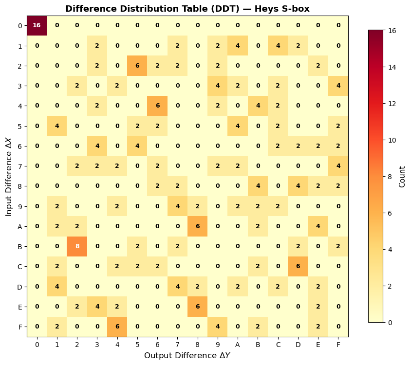
Cells with count >= 6 (strong differentials):
  Delta_X = 2h -> Delta_Y = 5h  (count=6, dp=0.3750)
  Delta_X = 4h -> Delta_Y = 6h  (count=6, dp=0.3750)
  Delta_X = Ah -> Delta_Y = 8h  (count=6, dp=0.3750)
  Delta_X = Bh -> Delta_Y = 2h  (count=8, dp=0.5000)
  Delta_X = Ch -> Delta_Y = Dh  (count=6, dp=0.3750)
  Delta_X = Eh -> Delta_Y = 8h  (count=6, dp=0.3750)
  Delta_X = Fh -> Delta_Y = 4h  (count=6, dp=0.3750)

Observation

The DDT reveals the differential structure of the S-box at a glance. The first row (input difference 0) concentrates entirely at output difference 0, as expected. The brightest non-trivial cells represent the most exploitable differentials. For the Heys S-box, several differentials have probability \(6/16 = 0.375\), which is substantially higher than the ideal \(1/16 \approx 0.0625\) for a random function. These high-probability differentials are the entry points for a differential cryptanalysis attack.

Experiment 2: Verifying Key Cancellation#

We experimentally confirm Theorem 19.1: the output difference \(S(X \oplus K) \oplus S(X' \oplus K)\) is independent of the key \(K\).

Show code cell source Hide code cell source

import numpy as np
import matplotlib.pyplot as plt

HEYS_SBOX = np.array([0xE, 0x4, 0xD, 0x1, 0x2, 0xF, 0xB, 0x8,
                       0x3, 0xA, 0x6, 0xC, 0x5, 0x9, 0x0, 0x7])

# Choose a specific input difference
delta_x = 0xB  # input difference 1011b

# For each key, compute the output difference distribution
print(f'Input difference: Delta_X = 0x{delta_x:X} ({delta_x:04b}b)')
print(f'Testing all 16 possible keys...\n')

all_distributions = []

for key in range(16):
    counts = np.zeros(16, dtype=int)
    for x in range(16):
        x_prime = x ^ delta_x
        # Keyed S-box: S(x XOR K) XOR S(x' XOR K)
        y = HEYS_SBOX[x ^ key]
        y_prime = HEYS_SBOX[x_prime ^ key]
        delta_y = int(y ^ y_prime)
        counts[delta_y] += 1
    all_distributions.append(counts)

# Check all distributions are identical
all_same = all(np.array_equal(all_distributions[0], d) for d in all_distributions)
print(f'All 16 keyed distributions identical: {all_same}')
print(f'\nDistribution for Delta_X = 0x{delta_x:X}:')
for dy in range(16):
    if all_distributions[0][dy] > 0:
        print(f'  Delta_Y = 0x{dy:X}: count = {all_distributions[0][dy]}, '
              f'dp = {float(all_distributions[0][dy]/16):.4f}')

# Visualize: overlay all 16 key distributions
fig, (ax1, ax2) = plt.subplots(1, 2, figsize=(13, 5))

# Left: all 16 keyed distributions superimposed
x_pos = np.arange(16)
for key in range(16):
    ax1.bar(x_pos + key * 0.05 - 0.4, all_distributions[key],
            width=0.05, alpha=0.6, color=plt.cm.tab20(key))

ax1.set_xlabel(r'Output Difference $\Delta Y$', fontsize=11)
ax1.set_ylabel('Count', fontsize=11)
ax1.set_title(f'Key Cancellation: All 16 Keys Superimposed\n'
              f'($\\Delta X$ = 0x{delta_x:X})', fontsize=12)
ax1.set_xticks(range(16))
ax1.set_xticklabels([f'{x:X}' for x in range(16)])
ax1.grid(True, alpha=0.3, axis='y')

# Right: compare unkeyed DDT row with keyed DDT row for random key
analyzer = DifferentialAnalyzer(HEYS_SBOX)
ddt_row = analyzer.ddt[delta_x]

ax2.bar(x_pos - 0.2, ddt_row, width=0.35, alpha=0.8,
        color='#2c3e50', label='Unkeyed DDT row')
ax2.bar(x_pos + 0.2, all_distributions[7], width=0.35, alpha=0.8,
        color='#e74c3c', label='Keyed (K=0x7)')

ax2.set_xlabel(r'Output Difference $\Delta Y$', fontsize=11)
ax2.set_ylabel('Count', fontsize=11)
ax2.set_title(f'Unkeyed vs. Keyed DDT Row\n($\\Delta X$ = 0x{delta_x:X})',
              fontsize=12)
ax2.set_xticks(range(16))
ax2.set_xticklabels([f'{x:X}' for x in range(16)])
ax2.legend(fontsize=10)
ax2.grid(True, alpha=0.3, axis='y')

plt.tight_layout()
plt.savefig('key_cancellation.png', dpi=150, bbox_inches='tight')
plt.show()

Input difference: Delta_X = 0xB (1011b)
Testing all 16 possible keys...

All 16 keyed distributions identical: True

Distribution for Delta_X = 0xB:
  Delta_Y = 0x2: count = 8, dp = 0.5000
  Delta_Y = 0x5: count = 2, dp = 0.1250
  Delta_Y = 0x7: count = 2, dp = 0.1250
  Delta_Y = 0xD: count = 2, dp = 0.1250
  Delta_Y = 0xF: count = 2, dp = 0.1250

../_images/cdd6181f5631fcf21470e1788d7315f4e79f75b18c79cbfc46c7c02f546b11fa.png

Observation

The key cancellation property is confirmed: all 16 possible keys produce exactly the same output difference distribution for a given input difference. The bars for all keys overlap perfectly. This is the fundamental reason why differential cryptanalysis works: the attacker can precompute the DDT of the unkeyed S-box and use it to predict the behavior of the keyed cipher.

Experiment 3: Comparing S-box Designs#

We compare the DDTs of three different S-box designs:

Heys tutorial S-box (educational, moderate resistance)
AES S-box (SubBytes, 8-bit, designed for near-optimal differential resistance)
Random permutation (baseline)

import numpy as np

# --- Define the three S-boxes ---

# 1. Heys S-box (4-bit)
HEYS_SBOX = np.array([0xE, 0x4, 0xD, 0x1, 0x2, 0xF, 0xB, 0x8,
                       0x3, 0xA, 0x6, 0xC, 0x5, 0x9, 0x0, 0x7])

# 2. AES S-box (8-bit) -- full 256-entry SubBytes table
AES_SBOX = np.array([
    0x63, 0x7C, 0x77, 0x7B, 0xF2, 0x6B, 0x6F, 0xC5,
    0x30, 0x01, 0x67, 0x2B, 0xFE, 0xD7, 0xAB, 0x76,
    0xCA, 0x82, 0xC9, 0x7D, 0xFA, 0x59, 0x47, 0xF0,
    0xAD, 0xD4, 0xA2, 0xAF, 0x9C, 0xA4, 0x72, 0xC0,
    0xB7, 0xFD, 0x93, 0x26, 0x36, 0x3F, 0xF7, 0xCC,
    0x34, 0xA5, 0xE5, 0xF1, 0x71, 0xD8, 0x31, 0x15,
    0x04, 0xC7, 0x23, 0xC3, 0x18, 0x96, 0x05, 0x9A,
    0x07, 0x12, 0x80, 0xE2, 0xEB, 0x27, 0xB2, 0x75,
    0x09, 0x83, 0x2C, 0x1A, 0x1B, 0x6E, 0x5A, 0xA0,
    0x52, 0x3B, 0xD6, 0xB3, 0x29, 0xE3, 0x2F, 0x84,
    0x53, 0xD1, 0x00, 0xED, 0x20, 0xFC, 0xB1, 0x5B,
    0x6A, 0xCB, 0xBE, 0x39, 0x4A, 0x4C, 0x58, 0xCF,
    0xD0, 0xEF, 0xAA, 0xFB, 0x43, 0x4D, 0x33, 0x85,
    0x45, 0xF9, 0x02, 0x7F, 0x50, 0x3C, 0x9F, 0xA8,
    0x51, 0xA3, 0x40, 0x8F, 0x92, 0x9D, 0x38, 0xF5,
    0xBC, 0xB6, 0xDA, 0x21, 0x10, 0xFF, 0xF3, 0xD2,
    0xCD, 0x0C, 0x13, 0xEC, 0x5F, 0x97, 0x44, 0x17,
    0xC4, 0xA7, 0x7E, 0x3D, 0x64, 0x5D, 0x19, 0x73,
    0x60, 0x81, 0x4F, 0xDC, 0x22, 0x2A, 0x90, 0x88,
    0x46, 0xEE, 0xB8, 0x14, 0xDE, 0x5E, 0x0B, 0xDB,
    0xE0, 0x32, 0x3A, 0x0A, 0x49, 0x06, 0x24, 0x5C,
    0xC2, 0xD3, 0xAC, 0x62, 0x91, 0x95, 0xE4, 0x79,
    0xE7, 0xC8, 0x37, 0x6D, 0x8D, 0xD5, 0x4E, 0xA9,
    0x6C, 0x56, 0xF4, 0xEA, 0x65, 0x7A, 0xAE, 0x08,
    0xBA, 0x78, 0x25, 0x2E, 0x1C, 0xA6, 0xB4, 0xC6,
    0xE8, 0xDD, 0x74, 0x1F, 0x4B, 0xBD, 0x8B, 0x8A,
    0x70, 0x3E, 0xB5, 0x66, 0x48, 0x03, 0xF6, 0x0E,
    0x61, 0x35, 0x57, 0xB9, 0x86, 0xC1, 0x1D, 0x9E,
    0xE1, 0xF8, 0x98, 0x11, 0x69, 0xD9, 0x8E, 0x94,
    0x9B, 0x1E, 0x87, 0xE9, 0xCE, 0x55, 0x28, 0xDF,
    0x8C, 0xA1, 0x89, 0x0D, 0xBF, 0xE6, 0x42, 0x68,
    0x41, 0x99, 0x2D, 0x0F, 0xB0, 0x54, 0xBB, 0x16,
], dtype=int)

# 3. Random 4-bit permutation (for comparison with Heys)
rng = np.random.default_rng(42)
RANDOM_SBOX_4 = rng.permutation(16).astype(int)

print('S-box definitions:')
print(f'  Heys:   {[hex(x) for x in HEYS_SBOX]}')
print(f'  AES:    [{hex(AES_SBOX[0])}, {hex(AES_SBOX[1])}, ..., '
      f'{hex(AES_SBOX[254])}, {hex(AES_SBOX[255])}] (256 entries)')
print(f'  Random: {[hex(x) for x in RANDOM_SBOX_4]}')

S-box definitions:
  Heys:   ['0xe', '0x4', '0xd', '0x1', '0x2', '0xf', '0xb', '0x8', '0x3', '0xa', '0x6', '0xc', '0x5', '0x9', '0x0', '0x7']
  AES:    [0x63, 0x7c, ..., 0xbb, 0x16] (256 entries)
  Random: ['0x6', '0xf', '0xb', '0xa', '0x9', '0x3', '0x0', '0x7', '0xc', '0x5', '0x2', '0x4', '0xe', '0x1', '0xd', '0x8']

Show code cell source Hide code cell source

import numpy as np
import matplotlib.pyplot as plt

# Redefine S-boxes for fresh imports
HEYS_SBOX = np.array([0xE, 0x4, 0xD, 0x1, 0x2, 0xF, 0xB, 0x8,
                       0x3, 0xA, 0x6, 0xC, 0x5, 0x9, 0x0, 0x7])

rng = np.random.default_rng(42)
RANDOM_SBOX_4 = rng.permutation(16).astype(int)

# Compute DDTs for the two 4-bit S-boxes
analyzer_heys = DifferentialAnalyzer(HEYS_SBOX)
analyzer_rand = DifferentialAnalyzer(RANDOM_SBOX_4)

ddt_heys = analyzer_heys.ddt
ddt_rand = analyzer_rand.ddt

fig, (ax1, ax2) = plt.subplots(1, 2, figsize=(14, 6))

# Heys DDT heatmap
im1 = ax1.imshow(ddt_heys, cmap='YlOrRd', aspect='equal', vmin=0, vmax=16)
for i in range(16):
    for j in range(16):
        val = ddt_heys[i, j]
        color = 'white' if val >= 8 else 'black'
        ax1.text(j, i, str(val), ha='center', va='center',
                fontsize=7, fontweight='bold', color=color)
ax1.set_xticks(range(16))
ax1.set_yticks(range(16))
ax1.set_xticklabels([f'{x:X}' for x in range(16)], fontsize=8)
ax1.set_yticklabels([f'{x:X}' for x in range(16)], fontsize=8)
ax1.set_xlabel(r'$\Delta Y$', fontsize=11)
ax1.set_ylabel(r'$\Delta X$', fontsize=11)
ax1.set_title(f'Heys S-box\nmax dp = {float(analyzer_heys.max_differential_probability()):.3f}',
              fontsize=12, fontweight='bold')

# Random DDT heatmap
im2 = ax2.imshow(ddt_rand, cmap='YlOrRd', aspect='equal', vmin=0, vmax=16)
for i in range(16):
    for j in range(16):
        val = ddt_rand[i, j]
        color = 'white' if val >= 8 else 'black'
        ax2.text(j, i, str(val), ha='center', va='center',
                fontsize=7, fontweight='bold', color=color)
ax2.set_xticks(range(16))
ax2.set_yticks(range(16))
ax2.set_xticklabels([f'{x:X}' for x in range(16)], fontsize=8)
ax2.set_yticklabels([f'{x:X}' for x in range(16)], fontsize=8)
ax2.set_xlabel(r'$\Delta Y$', fontsize=11)
ax2.set_ylabel(r'$\Delta X$', fontsize=11)
ax2.set_title(f'Random Permutation\nmax dp = {float(analyzer_rand.max_differential_probability()):.3f}',
              fontsize=12, fontweight='bold')

plt.colorbar(im1, ax=ax1, shrink=0.8, label='Count')
plt.colorbar(im2, ax=ax2, shrink=0.8, label='Count')

plt.tight_layout()
plt.savefig('ddt_comparison_4bit.png', dpi=150, bbox_inches='tight')
plt.show()

print(f'Heys S-box:  differential uniformity = {analyzer_heys.differential_uniformity()}, '
      f'max dp = {float(analyzer_heys.max_differential_probability()):.4f}')
print(f'Random perm: differential uniformity = {analyzer_rand.differential_uniformity()}, '
      f'max dp = {float(analyzer_rand.max_differential_probability()):.4f}')

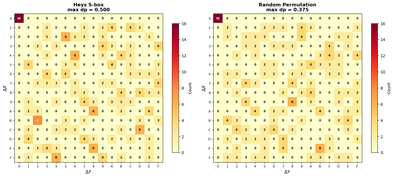
../_images/8b29d65e516ad75444d0cfad1c0d7c4890071d60fe9acbfabb12a69a9eaa0269.png

Heys S-box:  differential uniformity = 8, max dp = 0.5000
Random perm: differential uniformity = 6, max dp = 0.3750

Show code cell source Hide code cell source

import numpy as np
import matplotlib.pyplot as plt

# AES S-box DDT (8-bit: 256x256 table)
AES_SBOX = np.array([
    0x63, 0x7C, 0x77, 0x7B, 0xF2, 0x6B, 0x6F, 0xC5,
    0x30, 0x01, 0x67, 0x2B, 0xFE, 0xD7, 0xAB, 0x76,
    0xCA, 0x82, 0xC9, 0x7D, 0xFA, 0x59, 0x47, 0xF0,
    0xAD, 0xD4, 0xA2, 0xAF, 0x9C, 0xA4, 0x72, 0xC0,
    0xB7, 0xFD, 0x93, 0x26, 0x36, 0x3F, 0xF7, 0xCC,
    0x34, 0xA5, 0xE5, 0xF1, 0x71, 0xD8, 0x31, 0x15,
    0x04, 0xC7, 0x23, 0xC3, 0x18, 0x96, 0x05, 0x9A,
    0x07, 0x12, 0x80, 0xE2, 0xEB, 0x27, 0xB2, 0x75,
    0x09, 0x83, 0x2C, 0x1A, 0x1B, 0x6E, 0x5A, 0xA0,
    0x52, 0x3B, 0xD6, 0xB3, 0x29, 0xE3, 0x2F, 0x84,
    0x53, 0xD1, 0x00, 0xED, 0x20, 0xFC, 0xB1, 0x5B,
    0x6A, 0xCB, 0xBE, 0x39, 0x4A, 0x4C, 0x58, 0xCF,
    0xD0, 0xEF, 0xAA, 0xFB, 0x43, 0x4D, 0x33, 0x85,
    0x45, 0xF9, 0x02, 0x7F, 0x50, 0x3C, 0x9F, 0xA8,
    0x51, 0xA3, 0x40, 0x8F, 0x92, 0x9D, 0x38, 0xF5,
    0xBC, 0xB6, 0xDA, 0x21, 0x10, 0xFF, 0xF3, 0xD2,
    0xCD, 0x0C, 0x13, 0xEC, 0x5F, 0x97, 0x44, 0x17,
    0xC4, 0xA7, 0x7E, 0x3D, 0x64, 0x5D, 0x19, 0x73,
    0x60, 0x81, 0x4F, 0xDC, 0x22, 0x2A, 0x90, 0x88,
    0x46, 0xEE, 0xB8, 0x14, 0xDE, 0x5E, 0x0B, 0xDB,
    0xE0, 0x32, 0x3A, 0x0A, 0x49, 0x06, 0x24, 0x5C,
    0xC2, 0xD3, 0xAC, 0x62, 0x91, 0x95, 0xE4, 0x79,
    0xE7, 0xC8, 0x37, 0x6D, 0x8D, 0xD5, 0x4E, 0xA9,
    0x6C, 0x56, 0xF4, 0xEA, 0x65, 0x7A, 0xAE, 0x08,
    0xBA, 0x78, 0x25, 0x2E, 0x1C, 0xA6, 0xB4, 0xC6,
    0xE8, 0xDD, 0x74, 0x1F, 0x4B, 0xBD, 0x8B, 0x8A,
    0x70, 0x3E, 0xB5, 0x66, 0x48, 0x03, 0xF6, 0x0E,
    0x61, 0x35, 0x57, 0xB9, 0x86, 0xC1, 0x1D, 0x9E,
    0xE1, 0xF8, 0x98, 0x11, 0x69, 0xD9, 0x8E, 0x94,
    0x9B, 0x1E, 0x87, 0xE9, 0xCE, 0x55, 0x28, 0xDF,
    0x8C, 0xA1, 0x89, 0x0D, 0xBF, 0xE6, 0x42, 0x68,
    0x41, 0x99, 0x2D, 0x0F, 0xB0, 0x54, 0xBB, 0x16,
], dtype=int)

analyzer_aes = DifferentialAnalyzer(AES_SBOX)
ddt_aes = analyzer_aes.ddt

print(f'AES S-box: {analyzer_aes.n_inputs} inputs, {analyzer_aes.n_outputs} outputs')
print(f'DDT shape: {ddt_aes.shape}')
print(f'Differential uniformity: {analyzer_aes.differential_uniformity()}')
print(f'Max dp (excl. 0->0): {float(analyzer_aes.max_differential_probability()):.6f}')
print(f'Ideal dp for random 8-bit function: {float(1/256):.6f}')
print(f'Ratio to ideal: {float(analyzer_aes.max_differential_probability() / (1/256)):.1f}x')

# Visualize AES DDT as heatmap
fig, ax = plt.subplots(figsize=(9, 8))

# Exclude row 0 for better contrast
ddt_display = ddt_aes[1:, :].copy()

im = ax.imshow(ddt_display, cmap='YlOrRd', aspect='equal',
               vmin=0, vmax=4, interpolation='nearest')
ax.set_xlabel(r'Output Difference $\Delta Y$', fontsize=11)
ax.set_ylabel(r'Input Difference $\Delta X$ (1..255)', fontsize=11)
ax.set_title(f'AES S-box DDT (rows 1..255)\n'
             f'Differential uniformity = {analyzer_aes.differential_uniformity()}, '
             f'max dp = {float(analyzer_aes.max_differential_probability()):.4f}',
             fontsize=12, fontweight='bold')
plt.colorbar(im, ax=ax, shrink=0.8, label='Count')

plt.tight_layout()
plt.savefig('ddt_aes_sbox.png', dpi=150, bbox_inches='tight')
plt.show()

# Entry value distribution
nonzero_entries = ddt_aes[1:, :].ravel()  # exclude row 0
unique, counts = np.unique(nonzero_entries, return_counts=True)
print(f'\nDDT entry value distribution (rows 1..255):')
for val, cnt in zip(unique, counts):
    print(f'  Value {val}: appears {cnt} times ({float(cnt / len(nonzero_entries) * 100):.1f}%)')

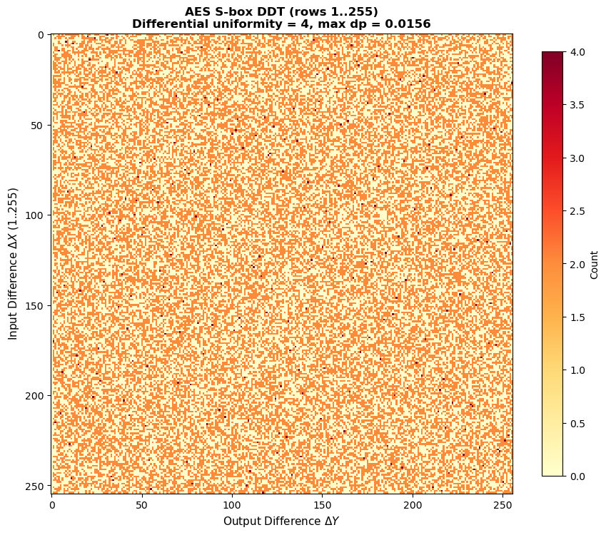
AES S-box: 256 inputs, 256 outputs
DDT shape: (256, 256)
Differential uniformity: 4
Max dp (excl. 0->0): 0.015625
Ideal dp for random 8-bit function: 0.003906
Ratio to ideal: 4.0x

../_images/043473c0905c0baad1db1ca08982e0fe836ae4c4a763fce882eb17e1819946c6.png

DDT entry value distribution (rows 1..255):
  Value 0: appears 32895 times (50.4%)
  Value 2: appears 32130 times (49.2%)
  Value 4: appears 255 times (0.4%)

Observation

The AES S-box achieves the theoretical minimum differential uniformity of 4 for an 8-bit S-box (it is an almost perfect nonlinear or APN-like function). This means the maximum differential probability is \(4/256 = 1/64 \approx 0.0156\), only 4 times the ideal bound of \(1/256\). By contrast, the Heys 4-bit S-box has differential uniformity 6, giving max dp \(= 6/16 = 0.375\), which is 6 times the ideal \(1/16\). The AES S-box is specifically constructed via the multiplicative inverse in \(\text{GF}(2^8)\) to achieve this near-optimal resistance.

Experiment 4: Distribution of Differential Probabilities#

We compare the histogram of DDT entry values across different S-box designs. An ideal S-box would have all non-trivial DDT entries as small and uniform as possible.

Show code cell source Hide code cell source

import numpy as np
import matplotlib.pyplot as plt

# Redefine S-boxes
HEYS_SBOX = np.array([0xE, 0x4, 0xD, 0x1, 0x2, 0xF, 0xB, 0x8,
                       0x3, 0xA, 0x6, 0xC, 0x5, 0x9, 0x0, 0x7])

rng = np.random.default_rng(42)
RANDOM_SBOX_4 = rng.permutation(16).astype(int)

# Compute DDTs
analyzer_heys = DifferentialAnalyzer(HEYS_SBOX)
analyzer_rand = DifferentialAnalyzer(RANDOM_SBOX_4)

# Also generate multiple random permutations and compute average statistics
n_random = 200
random_max_dps = []
random_uniformities = []

for seed in range(n_random):
    rng_i = np.random.default_rng(seed + 1000)
    rand_sbox = rng_i.permutation(16).astype(int)
    da = DifferentialAnalyzer(rand_sbox)
    random_max_dps.append(da.max_differential_probability())
    random_uniformities.append(da.differential_uniformity())

# Extract non-trivial DDT entries for histograms
ddt_heys = analyzer_heys.ddt.copy()
ddt_rand = analyzer_rand.ddt.copy()

# Exclude row 0 (trivial)
entries_heys = ddt_heys[1:, :].ravel()
entries_rand = ddt_rand[1:, :].ravel()

fig, axes = plt.subplots(1, 3, figsize=(16, 5))

# Panel 1: Histogram of DDT entries for Heys S-box
bins_4bit = np.arange(-0.5, 18.5, 1)
axes[0].hist(entries_heys, bins=bins_4bit, color='#2c3e50', alpha=0.8,
             edgecolor='white', linewidth=0.5)
axes[0].set_xlabel('DDT Entry Value', fontsize=11)
axes[0].set_ylabel('Frequency', fontsize=11)
axes[0].set_title(f'Heys S-box\nDiff. uniformity = {analyzer_heys.differential_uniformity()}',
                  fontsize=12, fontweight='bold')
axes[0].set_xticks(range(0, 18, 2))
axes[0].grid(True, alpha=0.3, axis='y')

# Panel 2: Histogram of DDT entries for random permutation
axes[1].hist(entries_rand, bins=bins_4bit, color='#e74c3c', alpha=0.8,
             edgecolor='white', linewidth=0.5)
axes[1].set_xlabel('DDT Entry Value', fontsize=11)
axes[1].set_ylabel('Frequency', fontsize=11)
axes[1].set_title(f'Random Permutation\nDiff. uniformity = {analyzer_rand.differential_uniformity()}',
                  fontsize=12, fontweight='bold')
axes[1].set_xticks(range(0, 18, 2))
axes[1].grid(True, alpha=0.3, axis='y')

# Panel 3: Distribution of max dp across 200 random 4-bit permutations
axes[2].hist(random_max_dps, bins=20, color='#3498db', alpha=0.8,
             edgecolor='white', linewidth=0.5)
axes[2].axvline(x=analyzer_heys.max_differential_probability(),
                color='#2c3e50', linestyle='--', linewidth=2,
                label=f'Heys max dp = {float(analyzer_heys.max_differential_probability()):.3f}')
axes[2].axvline(x=np.mean(random_max_dps), color='#e74c3c',
                linestyle=':', linewidth=2,
                label=f'Random mean = {float(np.mean(random_max_dps)):.3f}')
axes[2].set_xlabel('Maximum Differential Probability', fontsize=11)
axes[2].set_ylabel('Count (of 200 S-boxes)', fontsize=11)
axes[2].set_title('Max dp of 200 Random\n4-bit Permutations',
                  fontsize=12, fontweight='bold')
axes[2].legend(fontsize=9)
axes[2].grid(True, alpha=0.3, axis='y')

plt.tight_layout()
plt.savefig('dp_distribution_comparison.png', dpi=150, bbox_inches='tight')
plt.show()

print(f'Statistics over {n_random} random 4-bit permutations:')
print(f'  Mean max dp: {float(np.mean(random_max_dps)):.4f}')
print(f'  Std  max dp: {float(np.std(random_max_dps)):.4f}')
print(f'  Min  max dp: {float(np.min(random_max_dps)):.4f}')
print(f'  Max  max dp: {float(np.max(random_max_dps)):.4f}')
print(f'  Heys max dp: {float(analyzer_heys.max_differential_probability()):.4f}')
print(f'\nHeys S-box percentile among random: '
      f'{float(np.mean(np.array(random_max_dps) >= analyzer_heys.max_differential_probability()) * 100):.0f}%')

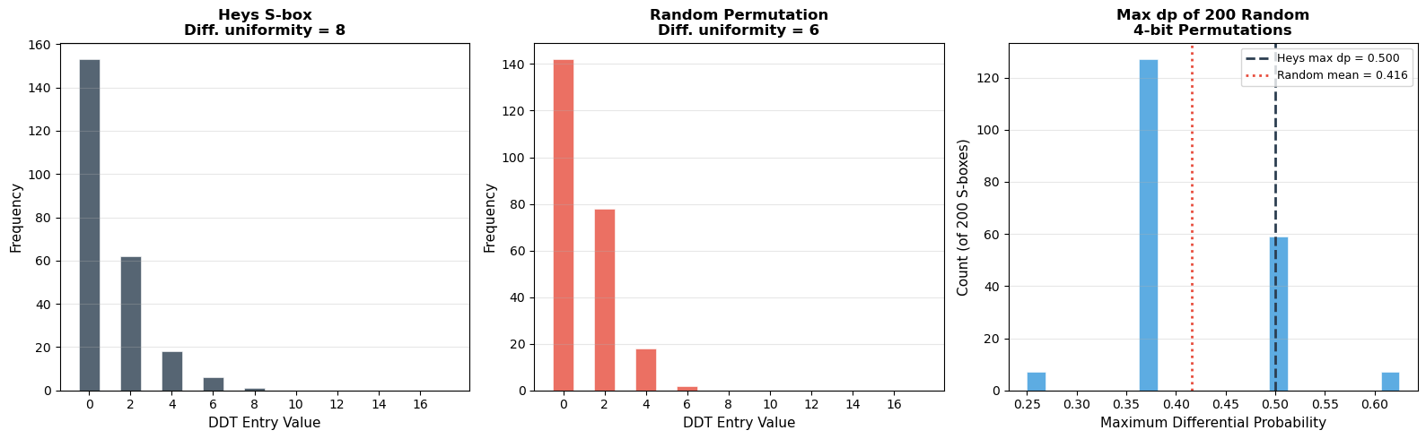
../_images/9ce771b0dd2432bf1a640eb1fa5ee1373b9ebd91eca010696958c4e3c2e773db.png

Statistics over 200 random 4-bit permutations:
  Mean max dp: 0.4163
  Std  max dp: 0.0751
  Min  max dp: 0.2500
  Max  max dp: 0.6250
  Heys max dp: 0.5000

Heys S-box percentile among random: 33%

Observation

The DDT entry histograms reveal the differential profile of each S-box. For the Heys S-box, most entries are 0 or 2, with occasional entries of 4 or 6. The random permutation shows a similar pattern, though its differential uniformity can vary. Comparing the Heys S-box against 200 random permutations shows that its max dp is typical of a random 4-bit permutation — at this small size, there is limited room for optimization. The real gains from careful S-box design appear at larger sizes (8 bits, as in AES), where the gap between optimal and random constructions is much larger.

19.5 Exercises#

Exercise 19.1 (Warm-up)#

For the Heys S-box, manually verify the DDT entry for \(\Delta X = 5\), \(\Delta Y = 9\). List all inputs \(X\) such that \(S(X) \oplus S(X \oplus 5) = 9\).

Hint

Iterate over all \(X \in \{0, 1, \ldots, 15\}\), compute \(X' = X \oplus 5\), then check whether \(S(X) \oplus S(X') = 9\). Remember that the S-box is [0xE, 0x4, 0xD, 0x1, 0x2, 0xF, 0xB, 0x8, 0x3, 0xA, 0x6, 0xC, 0x5, 0x9, 0x0, 0x7]. The count should match DDT[5][9].

Exercise 19.2 (Applied)#

Write a function that, given an S-box, determines whether it is a bijection (permutation) by checking both the standard definition (all outputs distinct) and the DDT structure (column sums all equal \(2^n\)). Verify your function on the Heys S-box and on the non-bijective mapping \(S(x) = x \mathbin{\&} \texttt{0x7}\) (bitwise AND masking the top bit).

Hint

For the bijection check: len(set(sbox)) == len(sbox). For the DDT check: compute the DDT and verify that all column sums equal \(2^n\). For a non-bijective function, the column sums will not all be equal (some output differences are more likely because the function is not injective).

Exercise 19.3 (Analysis)#

Prove that all entries in the DDT of any S-box are even. More precisely, show that the solutions to \(S(X) \oplus S(X \oplus \Delta X) = \Delta Y\) always come in pairs.

Hint

If \(X_0\) is a solution (i.e., \(S(X_0) \oplus S(X_0 \oplus \Delta X) = \Delta Y\)), then \(X_0' = X_0 \oplus \Delta X\) is also a solution: \(S(X_0') \oplus S(X_0' \oplus \Delta X) = S(X_0 \oplus \Delta X) \oplus S(X_0) = \Delta Y\). If \(\Delta X \neq 0\), then \(X_0 \neq X_0'\), so solutions come in distinct pairs.

Exercise 19.4 (Theory)#

An S-box \(S: \{0,1\}^n \to \{0,1\}^n\) is called almost perfect nonlinear (APN) if its differential uniformity is exactly 2 (the minimum possible for \(n > 1\)). Show that the AES S-box is not APN (its differential uniformity is 4). Explain why no 8-bit bijective S-box can be APN.

Hint

Compute the AES DDT and find the maximum entry. For the impossibility result: it has been proven that APN permutations of \(\{0,1\}^n\) exist only for odd \(n\). Since \(n = 8\) is even, no APN bijection on 8 bits exists. The best achievable differential uniformity for an 8-bit bijection is 4, which the AES S-box achieves.

Exercise 19.5 (Challenge)#

Search for the optimal 4-bit S-box: a permutation of \(\{0, \ldots, 15\}\) that minimizes the differential uniformity. Use a random search (generate 10,000 random permutations) and report:

The minimum differential uniformity found
How many of the 10,000 permutations achieve this minimum
A histogram of differential uniformities across all 10,000 permutations

Hint

For a 4-bit bijection, the minimum possible differential uniformity is 4 (since all DDT entries are even and each nonzero row sums to 16, there must be at least one entry \(\geq 4\) when entries are distributed among 16 columns with sum 16 and all entries even). Use np.random.default_rng().permutation(16) to generate candidates and DifferentialAnalyzer to evaluate each.

19.6 Summary#

Concept	Key Point
Differential cryptanalysis	Study how XOR differences propagate through a cipher
Input/output difference	\(\Delta X = X \oplus X'\), \(\Delta Y = S(X) \oplus S(X')\)
DDT	\(2^n \times 2^m\) table counting how often each \(\Delta X\) produces each \(\Delta Y\)
Differential probability	\(\text{dp}(\Delta X \to \Delta Y) = \text{DDT}[\Delta X][\Delta Y] / 2^n\)
Key cancellation	XOR key mixing does not affect input differences
DDT properties	Row/column sums \(= 2^n\); all entries even; first row concentrated at 0
Differential uniformity	Maximum DDT entry (excluding \(0 \to 0\)); lower is better
AES S-box	Differential uniformity 4 (optimal for 8-bit bijection)
Historical significance	NSA knew about differential cryptanalysis before DES was published

Tip

The DDT is the fundamental data structure of differential cryptanalysis. In Chapter 20, we will use these differential probabilities to construct differential characteristics that trace a high-probability difference path through multiple rounds of a block cipher. In Chapter 21, we will mount a complete differential attack on a reduced-round SPN cipher, using the Heys S-box DDT computed in this chapter to recover secret key bits.

References#

Biham, E. and Shamir, A. (1991). “Differential Cryptanalysis of DES-like Cryptosystems.” Journal of Cryptology, 4(1), 3–72. The foundational paper that introduced differential cryptanalysis to the public cryptographic community. Presents the first attack on DES faster than brute force (\(2^{47}\) chosen plaintexts for the full 16 rounds). [9]
Heys, H. M. (2002). “A Tutorial on Linear and Differential Cryptanalysis.” Cryptologia, 26(3), 189–221. The standard pedagogical reference for both linear and differential cryptanalysis. The 4-bit S-box and SPN cipher used throughout this chapter and the next two chapters are from this tutorial. [11]
Coppersmith, D. (1994). “The Data Encryption Standard (DES) and its Strength Against Attacks.” IBM Journal of Research and Development, 38(3), 243–250. Reveals that the DES design team was aware of differential cryptanalysis (which they called the “T-attack”) and designed the S-boxes specifically to resist it. [12]
Nyberg, K. (1994). “Differentially Uniform Mappings for Cryptography.” EUROCRYPT ‘93, LNCS 765, 55–64. Formalizes the concept of differential uniformity and establishes the connection between S-box design and resistance to differential cryptanalysis. [13]
Daemen, J. and Rijmen, V. (2002). The Design of Rijndael: AES – The Advanced Encryption Standard. Springer. Describes the design rationale for the AES S-box, including its construction via multiplicative inversion in \(\text{GF}(2^8)\) to achieve optimal differential and linear properties. [14]

Chapter 19 — Foundations of Differential Cryptanalysis

Contents

Chapter 19 — Foundations of Differential Cryptanalysis#

19.1 Historical Context#

19.2 Formal Definitions#

19.3 Implementation#

19.4 Experiments#

Experiment 1: DDT Heatmap Visualization#

Experiment 2: Verifying Key Cancellation#

Experiment 3: Comparing S-box Designs#

Experiment 4: Distribution of Differential Probabilities#

19.5 Exercises#

Exercise 19.1 (Warm-up)#

Exercise 19.2 (Applied)#

Exercise 19.3 (Analysis)#

Exercise 19.4 (Theory)#

Exercise 19.5 (Challenge)#

19.6 Summary#

References#