
Chapter 39 — Grover’s Search Algorithm#
“A fast quantum mechanical algorithm for database search.” — Lov Grover, Proceedings of the 28th Annual ACM Symposium on Theory of Computing, 1996
In this chapter we study Grover’s search algorithm, the most important quantum algorithm for symmetric cryptanalysis. Grover’s algorithm provides a quadratic speedup for unstructured search: finding a marked element among \(N\) items in \(O(\sqrt{N})\) queries rather than \(O(N)\). We simulate the algorithm classically for small search spaces, visualize the amplitude amplification mechanism, and quantify its impact on the effective security of symmetric ciphers such as AES.
39.1 Historical Context#
In 1994, Peter Shor published his celebrated algorithm for integer factorization and discrete logarithms on a quantum computer, threatening all public-key cryptography based on these problems. Two years later, Lov Grover (Bell Labs, 1996) showed that quantum computers also affect symmetric cryptography, though less dramatically.
Grover’s algorithm solves the unstructured search problem: given a function \(f : \{0,1\}^n \to \{0,1\}\) that evaluates to 1 on exactly one input \(x^*\) (the target), find \(x^*\). Classically, any algorithm requires \(\Theta(N)\) queries in the worst case, where \(N = 2^n\). Grover showed that a quantum computer needs only \(O(\sqrt{N})\) queries.
Year |
Milestone |
|---|---|
1994 |
Shor’s algorithm: exponential speedup for factoring |
1996 |
Grover’s algorithm: quadratic speedup for unstructured search |
1997 |
Bennett, Bernstein, Brassard, Vazirani prove \(\Omega(\sqrt{N})\) lower bound |
1998 |
Boyer, Brassard, H\u00f8yer, Tapp extend to unknown number of solutions |
2016 |
NIST begins post-quantum standardization, citing Grover’s impact |
Important
The direct cryptographic consequence: a brute-force key search over a \(k\)-bit key space is reduced from \(2^k\) operations to \(2^{k/2}\) quantum queries. AES-128 drops from 128-bit to 64-bit effective security, while AES-256 drops to 128-bit — still considered safe.
39.2 Formal Definitions#
Definition 39.1 — Quantum Oracle
The oracle (also called the phase oracle) for target \(x^*\) is the unitary operator \(U_f\) that flips the sign of the target state:
As a matrix, \(U_f = I - 2|x^*\rangle\langle x^*|\) is a reflection about the hyperplane orthogonal to \(|x^*\rangle\).
Definition 39.2 — Grover Diffusion Operator
The diffusion operator (also called the inversion about the mean) is:
where \(|s\rangle = \frac{1}{\sqrt{N}}\sum_{x=0}^{N-1}|x\rangle\) is the uniform superposition state. In matrix form, \(D_{ij} = \frac{2}{N} - \delta_{ij}\).
Definition 39.3 — Grover Iteration
One Grover iteration (or Grover step) consists of applying the oracle followed by the diffusion operator:
The full algorithm applies \(G\) repeatedly to the initial uniform superposition \(|s\rangle\), then measures.
Theorem 39.1 — Optimal Number of Iterations
For a search space of size \(N\) with exactly one marked element, the probability of measuring the target state is maximized after
iterations, yielding success probability \(\geq 1 - \frac{1}{N}\).
Theorem 39.2 — Geometric Interpretation
Let \(|w\rangle = |x^*\rangle\) be the target state and \(|w^\perp\rangle = \frac{1}{\sqrt{N-1}} \sum_{x \neq x^*} |x\rangle\). Then \(|s\rangle = \sin\theta\,|w\rangle + \cos\theta\,|w^\perp\rangle\) where \(\sin\theta = \frac{1}{\sqrt{N}}\). Each Grover iteration rotates the state by \(2\theta\) toward \(|w\rangle\) in the 2D plane spanned by \(\{|w\rangle, |w^\perp\rangle\}\).
39.3 Implementation#
We simulate Grover’s algorithm by representing the quantum state as a classical amplitude vector of length \(N = 2^n\). While a real quantum computer would use \(n\) qubits, our simulation explicitly tracks all \(N\) amplitudes, costing \(O(N)\) memory and \(O(N)\) time per iteration.
import numpy as np
import math

def build_oracle(N, target):
    """
    Build the phase oracle U_f = I - 2|target><target|.

    The oracle flips the sign of the amplitude at index `target`,
    leaving all other amplitudes unchanged.

    Parameters
    ----------
    N : int
        Size of the search space (must be a power of 2).
    target : int
        Index of the marked element (0 <= target < N).

    Returns
    -------
    oracle : ndarray of shape (N, N)
        Diagonal matrix with -1 at position (target, target), +1 elsewhere.
    """
    oracle = np.eye(N)
    oracle[target, target] = -1.0
    return oracle


def build_diffusion(N):
    """
    Build the Grover diffusion operator D = 2|s><s| - I.

    Parameters
    ----------
    N : int
        Size of the search space.

    Returns
    -------
    D : ndarray of shape (N, N)
        The diffusion matrix with D[i,j] = 2/N - delta_{ij}.
    """
    s = np.ones(N) / np.sqrt(N)           # uniform superposition
    D = 2.0 * np.outer(s, s) - np.eye(N)  # 2|s><s| - I
    return D


def grover_simulate(n_qubits, target, n_iterations=None):
    """
    Simulate Grover's algorithm and return the state after each iteration.

    Parameters
    ----------
    n_qubits : int
        Number of qubits. Search space size N = 2^n_qubits.
    target : int
        Index of the marked element.
    n_iterations : int or None
        Number of Grover iterations. If None, uses optimal count.

    Returns
    -------
    history : list of ndarray
        Amplitude vectors after each iteration (including initial state).
    """
    N = 2 ** n_qubits
    if n_iterations is None:
        n_iterations = int(np.floor(np.pi / 4 * np.sqrt(N)))

    oracle = build_oracle(N, target)
    diffusion = build_diffusion(N)
    grover_op = diffusion @ oracle       # G = D * U_f

    # Initial state: uniform superposition
    state = np.ones(N) / np.sqrt(N)
    history = [state.copy()]

    for _ in range(n_iterations):
        state = grover_op @ state
        history.append(state.copy())

    return history


# --- Demo: 3-qubit Grover search (N=8) ---
n_qubits = 3
N = 2 ** n_qubits
target = 5
t_opt = int(np.floor(np.pi / 4 * np.sqrt(N)))

print(f'Search space: N = {N}')
print(f'Target: |{target}> = |{target:0{n_qubits}b}>')
print(f'Optimal iterations: floor(pi/4 * sqrt({N})) = {t_opt}')

history = grover_simulate(n_qubits, target)

final_state = history[-1]
probs = final_state ** 2

print(f'\nAfter {t_opt} iterations:')
for i in range(N):
    marker = ' <-- TARGET' if i == target else ''
    print(f'  |{i:0{n_qubits}b}> : amplitude = {final_state[i]:+.4f}, '
          f'probability = {float(probs[i]):.4f}{marker}')
print(f'\nSuccess probability: {float(probs[target]):.6f}')
Search space: N = 8
Target: |5> = |101>
Optimal iterations: floor(pi/4 * sqrt(8)) = 2

After 2 iterations:
  |000> : amplitude = -0.0884, probability = 0.0078
  |001> : amplitude = -0.0884, probability = 0.0078
  |010> : amplitude = -0.0884, probability = 0.0078
  |011> : amplitude = -0.0884, probability = 0.0078
  |100> : amplitude = -0.0884, probability = 0.0078
  |101> : amplitude = +0.9723, probability = 0.9453 <-- TARGET
  |110> : amplitude = -0.0884, probability = 0.0078
  |111> : amplitude = -0.0884, probability = 0.0078

Success probability: 0.945312
Implementation Note
We represent the oracle as a diagonal matrix and the diffusion operator as a dense \(N \times N\) matrix. For production use, one would exploit the structure: the oracle is a single sign flip, and the diffusion operator can be applied in \(O(N)\) time via the identity \(D|\psi\rangle = -|\psi\rangle + \frac{2}{N}(\sum_i \psi_i)|s\rangle\), avoiding the \(O(N^2)\) cost of a full matrix-vector multiplication.
import numpy as np

def grover_simulate_fast(n_qubits, target, n_iterations=None):
    """
    Memory-efficient Grover simulation without building full matrices.

    Instead of matrix-vector products, we apply the oracle and diffusion
    operator directly on the amplitude vector:
      - Oracle: negate amplitude at target index.           O(1)
      - Diffusion: psi -> -psi + (2/N) * sum(psi) * ones.  O(N)

    Total cost: O(N) per iteration instead of O(N^2).
    """
    N = 2 ** n_qubits
    if n_iterations is None:
        n_iterations = int(np.floor(np.pi / 4 * np.sqrt(N)))

    state = np.ones(N) / np.sqrt(N)
    history = [state.copy()]

    for _ in range(n_iterations):
        # Oracle: flip sign of target
        state[target] *= -1.0
        # Diffusion: inversion about the mean
        mean_amp = np.mean(state)
        state = 2.0 * mean_amp - state
        history.append(state.copy())

    return history


# Verify both implementations agree
n_qubits = 4
target = 11
N = 2 ** n_qubits

hist_full = grover_simulate(n_qubits, target)
hist_fast = grover_simulate_fast(n_qubits, target)

print(f'Verification (n={n_qubits}, N={N}, target={target}):')
for step in range(len(hist_full)):
    diff = np.max(np.abs(hist_full[step] - hist_fast[step]))
    print(f'  Step {step}: max difference = {diff:.2e}')

print(f'\nFinal success probability (full):  {float(hist_full[-1][target]**2):.6f}')
print(f'Final success probability (fast):  {float(hist_fast[-1][target]**2):.6f}')
Verification (n=4, N=16, target=11):
  Step 0: max difference = 0.00e+00
  Step 1: max difference = 0.00e+00
  Step 2: max difference = 0.00e+00
  Step 3: max difference = 0.00e+00

Final success probability (full):  0.961319
Final success probability (fast):  0.961319
39.4 Geometric Visualization#
Grover’s algorithm can be understood geometrically as a rotation in a 2D plane. The entire \(N\)-dimensional Hilbert space is reduced to just two relevant directions: the target state \(|w\rangle\) and the uniform superposition of all non-target states \(|w^\perp\rangle\).
Show code cell source
import numpy as np
import matplotlib.pyplot as plt
import math

def plot_grover_geometry(n_qubits, target):
    """
    Visualize Grover's algorithm as rotation in the |w>, |w_perp> plane.
    """
    N = 2 ** n_qubits
    theta = np.arcsin(1.0 / np.sqrt(N))  # initial angle
    t_opt = int(np.floor(np.pi / 4 * np.sqrt(N)))

    fig, ax = plt.subplots(figsize=(7, 7))

    # Draw unit circle (first quadrant)
    angles_circle = np.linspace(0, np.pi / 2, 200)
    ax.plot(np.cos(angles_circle), np.sin(angles_circle),
            'k-', alpha=0.15, linewidth=1)

    # Draw axes
    ax.annotate('', xy=(1.15, 0), xytext=(0, 0),
                arrowprops=dict(arrowstyle='->', color='black', lw=1.5))
    ax.annotate('', xy=(0, 1.15), xytext=(0, 0),
                arrowprops=dict(arrowstyle='->', color='black', lw=1.5))
    ax.text(1.18, -0.04, r'$|w^\perp\rangle$', fontsize=14)
    ax.text(-0.12, 1.15, r'$|w\rangle$', fontsize=14)

    # Plot state evolution
    colors = plt.cm.viridis(np.linspace(0.1, 0.9, t_opt + 1))

    for step in range(t_opt + 1):
        angle = (2 * step + 1) * theta
        x_coord = np.cos(angle)
        y_coord = np.sin(angle)

        ax.annotate('',
                    xy=(x_coord, y_coord), xytext=(0, 0),
                    arrowprops=dict(arrowstyle='->', color=colors[step],
                                   lw=2.0, alpha=0.8))

        label_r = 1.08
        ax.text(label_r * np.cos(angle), label_r * np.sin(angle),
                f't={step}', fontsize=9, ha='center', va='center',
                color=colors[step], fontweight='bold')

    # Mark initial angle
    arc_angles = np.linspace(0, theta, 50)
    arc_r = 0.35
    ax.plot(arc_r * np.cos(arc_angles), arc_r * np.sin(arc_angles),
            'r-', linewidth=1.5)
    ax.text(arc_r * np.cos(theta / 2) + 0.05,
            arc_r * np.sin(theta / 2) + 0.03,
            r'$\theta$', fontsize=13, color='red')

    # Mark rotation step
    arc2_angles = np.linspace(theta, 3 * theta, 50)
    arc2_r = 0.55
    ax.plot(arc2_r * np.cos(arc2_angles), arc2_r * np.sin(arc2_angles),
            'b-', linewidth=1.5)
    mid_angle = 2 * theta
    ax.text(arc2_r * np.cos(mid_angle) + 0.07,
            arc2_r * np.sin(mid_angle),
            r'$2\theta$', fontsize=13, color='blue')

    ax.set_xlim(-0.15, 1.35)
    ax.set_ylim(-0.15, 1.35)
    ax.set_aspect('equal')
    ax.set_title(f'Grover rotation for N={N} (n={n_qubits} qubits)\n'
                 f'$\\theta$ = arcsin(1/$\\sqrt{{{N}}}$) = {float(np.degrees(theta)):.1f}$^\\circ$, '
                 f'optimal iterations = {t_opt}',
                 fontsize=12)
    ax.grid(True, alpha=0.2)

    plt.tight_layout()
    plt.savefig('grover_geometry.png', dpi=150, bbox_inches='tight')
    plt.show()


plot_grover_geometry(n_qubits=3, target=5)
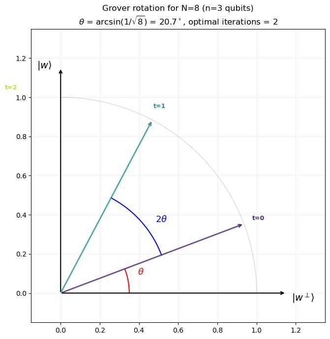
Tip
The geometric picture makes it clear why too many iterations decrease the success probability: the state vector rotates past \(|w\rangle\) and starts moving away from it. This is a key difference from classical search, where more work never hurts.
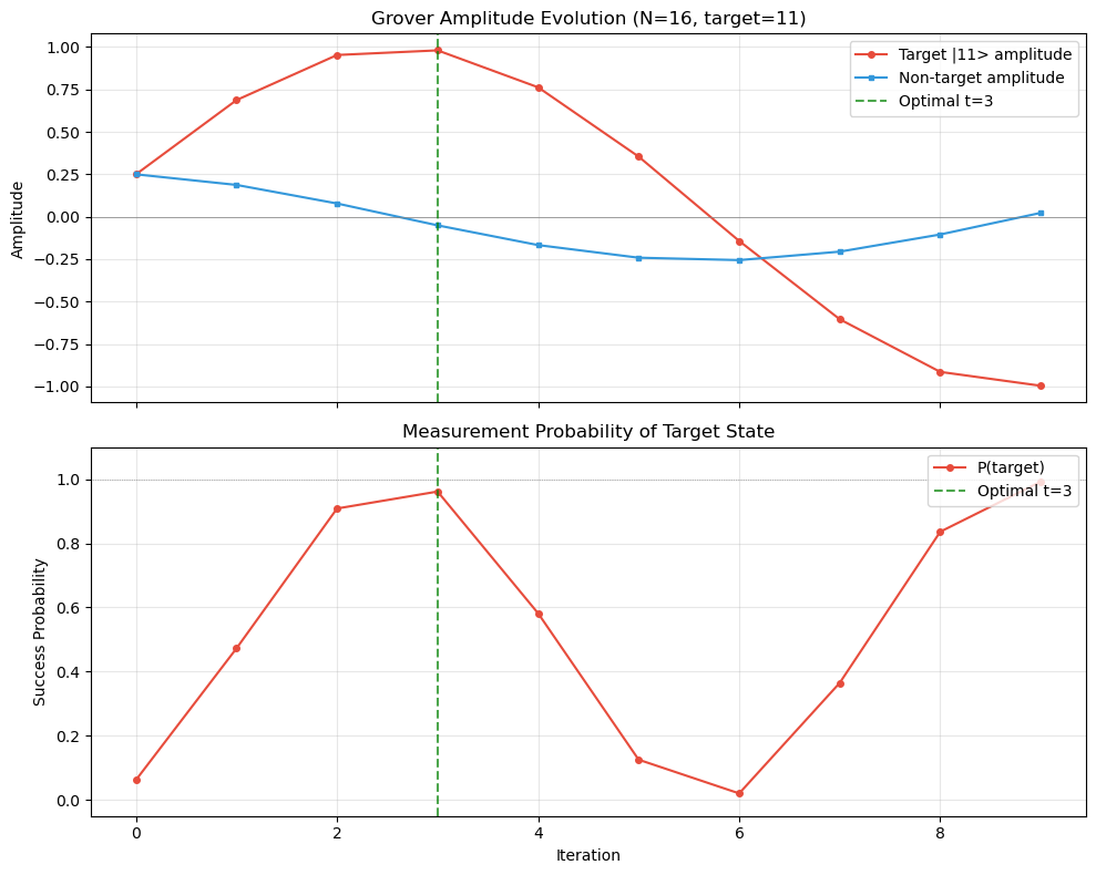
Show code cell source
import numpy as np
import matplotlib.pyplot as plt
import math

def plot_amplitude_evolution(n_qubits, target, max_iters=None):
    """
    Show how amplitudes of the target and non-target states evolve
    over Grover iterations.
    """
    N = 2 ** n_qubits
    t_opt = int(np.floor(np.pi / 4 * np.sqrt(N)))
    if max_iters is None:
        max_iters = 3 * t_opt  # show overshooting behavior

    history = grover_simulate_fast(n_qubits, target, n_iterations=max_iters)

    target_amps = [h[target] for h in history]
    other_amps = [h[0] if target != 0 else h[1] for h in history]
    target_probs = [a ** 2 for a in target_amps]

    steps = np.arange(len(history))

    fig, (ax1, ax2) = plt.subplots(2, 1, figsize=(10, 8), sharex=True)

    # Amplitudes
    ax1.plot(steps, target_amps, 'o-', color='#e74c3c', markersize=4,
             label=f'Target |{target}> amplitude')
    ax1.plot(steps, other_amps, 's-', color='#3498db', markersize=3,
             label='Non-target amplitude')
    ax1.axhline(y=0, color='gray', linewidth=0.5)
    ax1.axvline(x=t_opt, color='green', linestyle='--', alpha=0.7,
                label=f'Optimal t={t_opt}')
    ax1.set_ylabel('Amplitude')
    ax1.set_title(f'Grover Amplitude Evolution (N={N}, target={target})')
    ax1.legend(loc='upper right')
    ax1.grid(True, alpha=0.3)

    # Probabilities
    ax2.plot(steps, target_probs, 'o-', color='#e74c3c', markersize=4,
             label='P(target)')
    ax2.axhline(y=1.0, color='gray', linewidth=0.5, linestyle=':')
    ax2.axvline(x=t_opt, color='green', linestyle='--', alpha=0.7,
                label=f'Optimal t={t_opt}')
    ax2.set_xlabel('Iteration')
    ax2.set_ylabel('Success Probability')
    ax2.set_title('Measurement Probability of Target State')
    ax2.legend(loc='upper right')
    ax2.grid(True, alpha=0.3)
    ax2.set_ylim(-0.05, 1.1)

    plt.tight_layout()
    plt.savefig('grover_amplitude_evolution.png', dpi=150, bbox_inches='tight')
    plt.show()


plot_amplitude_evolution(n_qubits=4, target=11)
39.5 Experiments#
Experiment 1: Success Probability vs. Iterations for N = 8, 16, 32#
We run Grover’s algorithm for three search space sizes and plot the success probability as a function of the number of iterations, confirming the periodic behavior and the optimal stopping point.
Show code cell source
import numpy as np
import matplotlib.pyplot as plt
import math

fig, axes = plt.subplots(1, 3, figsize=(15, 5))

configs = [
    (3, 8, 5),    # (n_qubits, N, target)
    (4, 16, 11),
    (5, 32, 23),
]

for ax, (n_qubits, N, target) in zip(axes, configs):
    t_opt = int(np.floor(np.pi / 4 * np.sqrt(N)))
    max_iters = 4 * t_opt

    history = grover_simulate_fast(n_qubits, target, n_iterations=max_iters)
    probs = [h[target] ** 2 for h in history]
    steps = np.arange(len(history))

    ax.bar(steps, probs, color='#3498db', alpha=0.7, width=0.8)
    ax.axvline(x=t_opt, color='#e74c3c', linestyle='--', linewidth=2,
               label=f'$t_{{opt}}$ = {t_opt}')

    # Analytical prediction
    theta = np.arcsin(1.0 / np.sqrt(N))
    analytical = np.sin((2 * steps + 1) * theta) ** 2
    ax.plot(steps, analytical, 'r-', linewidth=1.5, alpha=0.8,
            label=r'$\sin^2((2t+1)\theta)$')

    ax.set_xlabel('Iteration $t$')
    ax.set_ylabel('P(target)')
    ax.set_title(f'N = {N} ({n_qubits} qubits)')
    ax.set_ylim(0, 1.15)
    ax.legend(fontsize=9)
    ax.grid(True, alpha=0.3)

    print(f'N={N}: t_opt={t_opt}, P(target)={float(probs[t_opt]):.6f}, '
          f'theta={float(np.degrees(theta)):.2f} deg')

fig.suptitle("Grover's Algorithm: Success Probability vs. Iterations",
             fontsize=14, y=1.02)
plt.tight_layout()
plt.savefig('grover_prob_vs_iters.png', dpi=150, bbox_inches='tight')
plt.show()
N=8: t_opt=2, P(target)=0.945312, theta=20.70 deg
N=16: t_opt=3, P(target)=0.961319, theta=14.48 deg
N=32: t_opt=4, P(target)=0.999182, theta=10.18 deg
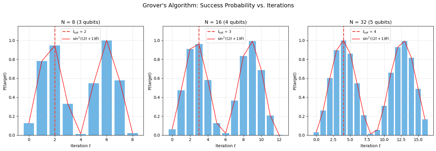
Observation
The success probability follows \(\sin^2((2t+1)\theta)\) exactly, confirming the geometric rotation model. Key observations:
For \(N=8\): the optimum is \(t=2\) with probability \(\approx 0.945\).
For \(N=16\): the optimum is \(t=3\) with probability \(\approx 0.961\).
For \(N=32\): the optimum is \(t=4\) with probability \(\approx 0.999\).
As \(N\) grows, the optimal success probability approaches 1, but overshooting becomes increasingly costly.
Experiment 2: Quantum vs. Classical Query Complexity#
We compare the number of oracle queries needed by Grover’s algorithm with the expected number needed by classical brute-force search.
Show code cell source
import numpy as np
import matplotlib.pyplot as plt
import math

n_qubits_range = np.arange(2, 21)
N_values = 2 ** n_qubits_range

# Classical: expected N/2 queries for brute force
classical_queries = N_values / 2.0

# Quantum: pi/4 * sqrt(N) Grover iterations
grover_queries = np.floor(np.pi / 4 * np.sqrt(N_values.astype(float)))

# Speedup factor
speedup = classical_queries / grover_queries

fig, (ax1, ax2) = plt.subplots(1, 2, figsize=(14, 5))

# Log-scale comparison
ax1.semilogy(n_qubits_range, classical_queries, 'o-', color='#e74c3c',
             label='Classical (N/2)', markersize=5)
ax1.semilogy(n_qubits_range, grover_queries, 's-', color='#3498db',
             label=r'Grover ($\pi/4 * \sqrt{N}$)', markersize=5)
ax1.set_xlabel('Number of qubits $n$')
ax1.set_ylabel('Oracle queries (log scale)')
ax1.set_title('Query Complexity: Classical vs. Grover')
ax1.legend(fontsize=11)
ax1.grid(True, alpha=0.3)

# Speedup factor
ax2.plot(n_qubits_range, speedup, 'o-', color='#2ecc71', markersize=5)
ax2.set_xlabel('Number of qubits $n$')
ax2.set_ylabel('Speedup factor (classical / quantum)')
ax2.set_title('Grover Speedup Factor')
ax2.grid(True, alpha=0.3)

# Annotate a few points
for n_q in [5, 10, 15, 20]:
    idx = n_q - 2
    ax2.annotate(f'{float(speedup[idx]):.0f}x',
                 xy=(n_q, speedup[idx]),
                 xytext=(n_q + 0.5, speedup[idx] + 10),
                 fontsize=9, color='#27ae60')

plt.tight_layout()
plt.savefig('grover_vs_classical.png', dpi=150, bbox_inches='tight')
plt.show()

# Print table
print(f'{"n":>4} {"N":>12} {"Classical":>14} {"Grover":>10} {"Speedup":>10}')
print('=' * 55)
for i, n_q in enumerate(n_qubits_range):
    print(f'{n_q:>4} {N_values[i]:>12} {float(classical_queries[i]):>14.0f} '
          f'{float(grover_queries[i]):>10.0f} {float(speedup[i]):>10.1f}x')
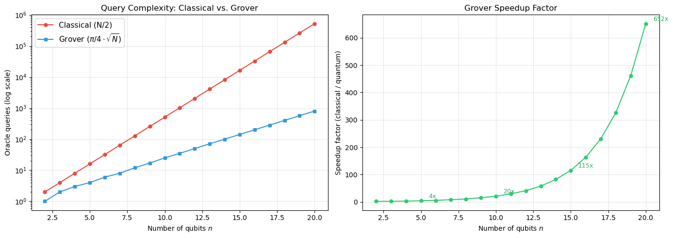
   n            N      Classical     Grover    Speedup
=======================================================
   2            4              2          1        2.0x
   3            8              4          2        2.0x
   4           16              8          3        2.7x
   5           32             16          4        4.0x
   6           64             32          6        5.3x
   7          128             64          8        8.0x
   8          256            128         12       10.7x
   9          512            256         17       15.1x
  10         1024            512         25       20.5x
  11         2048           1024         35       29.3x
  12         4096           2048         50       41.0x
  13         8192           4096         71       57.7x
  14        16384           8192        100       81.9x
  15        32768          16384        142      115.4x
  16        65536          32768        201      163.0x
  17       131072          65536        284      230.8x
  18       262144         131072        402      326.0x
  19       524288         262144        568      461.5x
  20      1048576         524288        804      652.1x
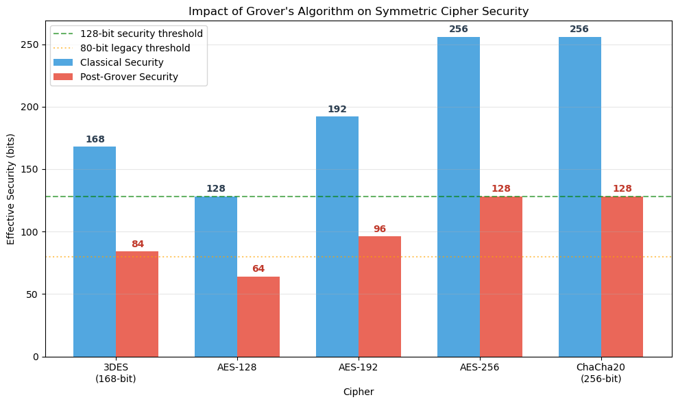
Experiment 3: Impact on AES Key Lengths#
Grover’s algorithm effectively halves the security level of symmetric ciphers. Here we quantify the impact on all three AES key sizes.
Show code cell source
import numpy as np
import matplotlib.pyplot as plt
import math

# AES key length impact table
print('Impact of Grover\'s Algorithm on AES Key Security')
print('=' * 72)
print(f'{"Cipher":<12} {"Key bits":<10} {"Classical":>14} {"Quantum":>14} {"Post-Quantum":>14}')
print(f'{"":<12} {"":<10} {"Security":>14} {"Security":>14} {"Recommendation":>14}')
print('-' * 72)

aes_configs = [
    ('AES-128', 128),
    ('AES-192', 192),
    ('AES-256', 256),
]

recommendations = {
    128: 'Upgrade to 256',
    192: 'Marginal',
    256: 'Safe (128-bit)',
}

for name, key_bits in aes_configs:
    classical_sec = key_bits
    quantum_sec = key_bits // 2
    rec = recommendations[key_bits]
    print(f'{name:<12} {key_bits:<10} {classical_sec:>14}-bit {quantum_sec:>11}-bit {rec:>14}')

print('-' * 72)
print(f'{"3DES":<12} {168:<10} {168:>14}-bit {84:>11}-bit {"Retire":>14}')
print(f'{"ChaCha20":<12} {256:<10} {256:>14}-bit {128:>11}-bit {"Safe (128-bit)":>14}')
print()

# Visualization
ciphers = ['3DES\n(168-bit)', 'AES-128', 'AES-192', 'AES-256', 'ChaCha20\n(256-bit)']
key_bits_list = [168, 128, 192, 256, 256]
classical_sec = key_bits_list
quantum_sec = [k // 2 for k in key_bits_list]

x = np.arange(len(ciphers))
width = 0.35

fig, ax = plt.subplots(figsize=(10, 6))
bars1 = ax.bar(x - width/2, classical_sec, width, label='Classical Security',
               color='#3498db', alpha=0.85)
bars2 = ax.bar(x + width/2, quantum_sec, width, label='Post-Grover Security',
               color='#e74c3c', alpha=0.85)

# Security threshold lines
ax.axhline(y=128, color='green', linestyle='--', alpha=0.6,
           label='128-bit security threshold')
ax.axhline(y=80, color='orange', linestyle=':', alpha=0.6,
           label='80-bit legacy threshold')

ax.set_xlabel('Cipher')
ax.set_ylabel('Effective Security (bits)')
ax.set_title('Impact of Grover\'s Algorithm on Symmetric Cipher Security')
ax.set_xticks(x)
ax.set_xticklabels(ciphers)
ax.legend(loc='upper left')
ax.grid(True, axis='y', alpha=0.3)

# Add value labels on bars
for bar in bars1:
    height = bar.get_height()
    ax.text(bar.get_x() + bar.get_width()/2., height + 2,
            f'{int(height)}', ha='center', va='bottom', fontsize=10,
            fontweight='bold', color='#2c3e50')

for bar in bars2:
    height = bar.get_height()
    ax.text(bar.get_x() + bar.get_width()/2., height + 2,
            f'{int(height)}', ha='center', va='bottom', fontsize=10,
            fontweight='bold', color='#c0392b')

plt.tight_layout()
plt.savefig('grover_aes_impact.png', dpi=150, bbox_inches='tight')
plt.show()
Impact of Grover's Algorithm on AES Key Security
========================================================================
Cipher       Key bits        Classical        Quantum   Post-Quantum
                              Security       Security Recommendation
------------------------------------------------------------------------
AES-128      128                   128-bit          64-bit Upgrade to 256
AES-192      192                   192-bit          96-bit       Marginal
AES-256      256                   256-bit         128-bit Safe (128-bit)
------------------------------------------------------------------------
3DES         168                   168-bit          84-bit         Retire
ChaCha20     256                   256-bit         128-bit Safe (128-bit)
Danger
AES-128 drops to only 64-bit effective security under Grover’s algorithm. While no quantum computer capable of running Grover on 128-qubit search spaces exists today, NIST’s post-quantum guidelines recommend AES-256 for long-term security. AES-256 retains 128-bit quantum security, which matches today’s classical security standards.
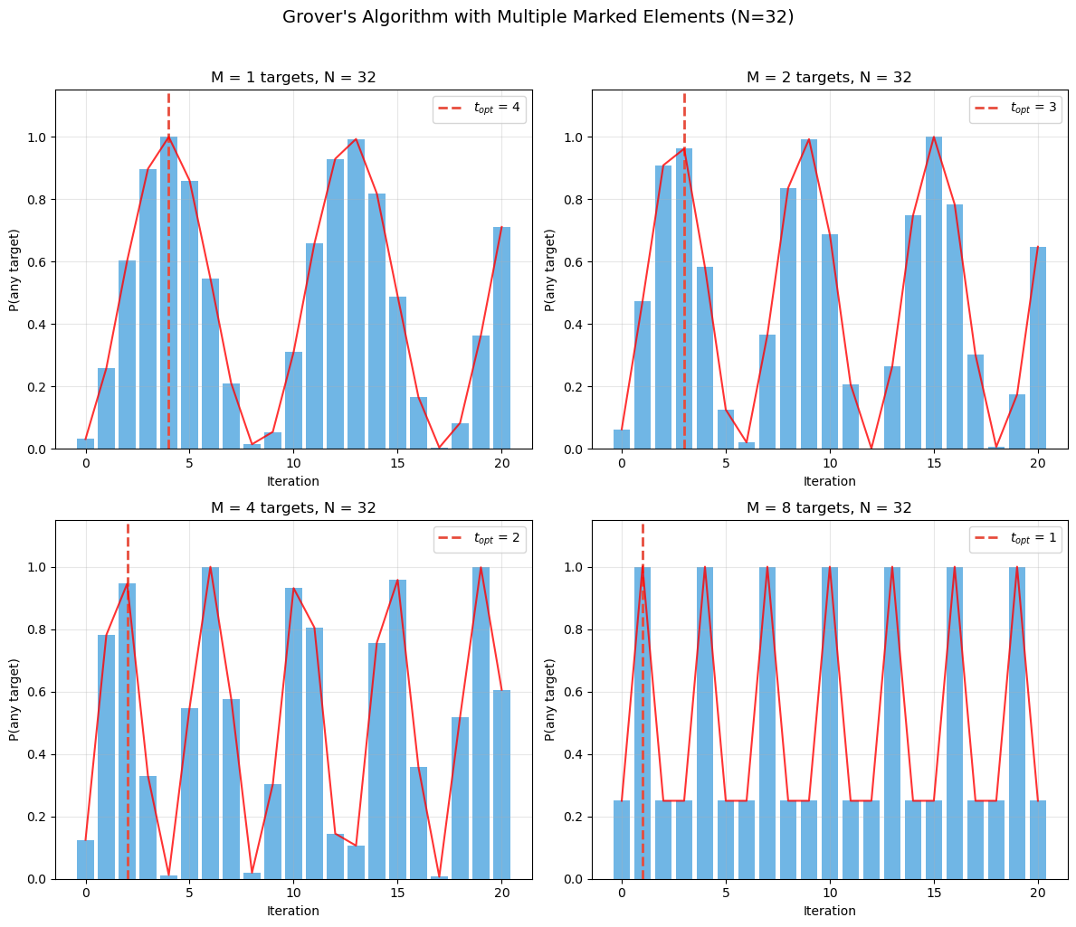
Experiment 4: Multiple Marked Elements#
When the oracle marks \(M\) out of \(N\) elements, the optimal number of iterations drops to \(\lfloor \frac{\pi}{4}\sqrt{N/M} \rfloor\). We verify this generalization.
Show code cell source
import numpy as np
import matplotlib.pyplot as plt
import math

def grover_multi_target(n_qubits, targets, n_iterations=None):
    """
    Simulate Grover with multiple marked elements.

    Parameters
    ----------
    n_qubits : int
        Number of qubits.
    targets : list of int
        Indices of marked elements.
    n_iterations : int or None
        Number of iterations. If None, uses optimal count.

    Returns
    -------
    history : list of ndarray
        Amplitude vectors after each iteration.
    """
    N = 2 ** n_qubits
    M = len(targets)
    if n_iterations is None:
        n_iterations = int(np.floor(np.pi / 4 * np.sqrt(N / M)))

    state = np.ones(N) / np.sqrt(N)
    history = [state.copy()]

    for _ in range(n_iterations):
        # Oracle: flip sign of all targets
        for t in targets:
            state[t] *= -1.0
        # Diffusion
        mean_amp = np.mean(state)
        state = 2.0 * mean_amp - state
        history.append(state.copy())

    return history


n_qubits = 5
N = 2 ** n_qubits  # N = 32

M_values = [1, 2, 4, 8]
rng = np.random.default_rng(42)

fig, axes = plt.subplots(2, 2, figsize=(12, 10))

for ax, M in zip(axes.flat, M_values):
    targets = sorted(rng.choice(N, size=M, replace=False).tolist())
    t_opt = int(np.floor(np.pi / 4 * np.sqrt(N / M)))
    max_iters = max(4 * t_opt, 20)

    history = grover_multi_target(n_qubits, targets, n_iterations=max_iters)

    # Total probability of measuring any target
    total_probs = [sum(h[t] ** 2 for t in targets) for h in history]
    steps = np.arange(len(history))

    ax.bar(steps, total_probs, color='#3498db', alpha=0.7, width=0.8)
    ax.axvline(x=t_opt, color='#e74c3c', linestyle='--', linewidth=2,
               label=f'$t_{{opt}}$ = {t_opt}')

    # Analytical
    theta = np.arcsin(np.sqrt(M / N))
    analytical = np.sin((2 * steps + 1) * theta) ** 2
    ax.plot(steps, analytical, 'r-', linewidth=1.5, alpha=0.8)

    ax.set_xlabel('Iteration')
    ax.set_ylabel('P(any target)')
    ax.set_title(f'M = {M} targets, N = {N}')
    ax.set_ylim(0, 1.15)
    ax.legend()
    ax.grid(True, alpha=0.3)

    print(f'M={M}: t_opt={t_opt}, P(success)={float(total_probs[t_opt]):.4f}, '
          f'targets={targets}')

fig.suptitle("Grover's Algorithm with Multiple Marked Elements (N=32)",
             fontsize=14, y=1.02)
plt.tight_layout()
plt.savefig('grover_multi_target.png', dpi=150, bbox_inches='tight')
plt.show()
M=1: t_opt=4, P(success)=0.9992, targets=[2]
M=2: t_opt=3, P(success)=0.9613, targets=[20, 23]
M=4: t_opt=2, P(success)=0.9453, targets=[2, 12, 22, 25]
M=8: t_opt=1, P(success)=1.0000, targets=[3, 15, 19, 20, 22, 24, 26, 27]
Experiment 5: Amplitude Bar Charts at Key Iterations#
We visualize the full amplitude distribution at several key moments during Grover’s algorithm to see the amplitude amplification in action.
Show code cell source
import numpy as np
import matplotlib.pyplot as plt
import math

n_qubits = 4
N = 2 ** n_qubits  # N = 16
target = 7
t_opt = int(np.floor(np.pi / 4 * np.sqrt(N)))

# Run for enough iterations to show full cycle
max_iters = 2 * t_opt + 2
history = grover_simulate_fast(n_qubits, target, n_iterations=max_iters)

# Select key iterations to display
display_iters = [0, 1, 2, t_opt, t_opt + 2, 2 * t_opt]
display_iters = [t for t in display_iters if t < len(history)]

fig, axes = plt.subplots(2, 3, figsize=(15, 8))

for ax, t in zip(axes.flat, display_iters):
    amps = history[t]
    colors = ['#e74c3c' if i == target else '#3498db' for i in range(N)]

    ax.bar(range(N), amps, color=colors, alpha=0.8)
    ax.axhline(y=0, color='gray', linewidth=0.5)
    ax.axhline(y=1.0 / np.sqrt(N), color='green', linewidth=0.8,
               linestyle=':', alpha=0.6, label=f'1/sqrt({N})')

    p_target = amps[target] ** 2
    ax.set_title(f'Iteration t={t}\nP(target)={float(p_target):.4f}', fontsize=11)
    ax.set_xlabel('State index')
    ax.set_ylabel('Amplitude')
    ax.set_ylim(-0.5, 1.1)
    ax.set_xticks(range(0, N, 2))
    ax.grid(True, alpha=0.2)

# Handle any unused axes
for idx in range(len(display_iters), len(axes.flat)):
    axes.flat[idx].set_visible(False)

fig.suptitle(f'Amplitude Distribution Evolution (N={N}, target={target}, '
             f't_opt={t_opt})', fontsize=13, y=1.02)
plt.tight_layout()
plt.savefig('grover_amplitude_bars.png', dpi=150, bbox_inches='tight')
plt.show()
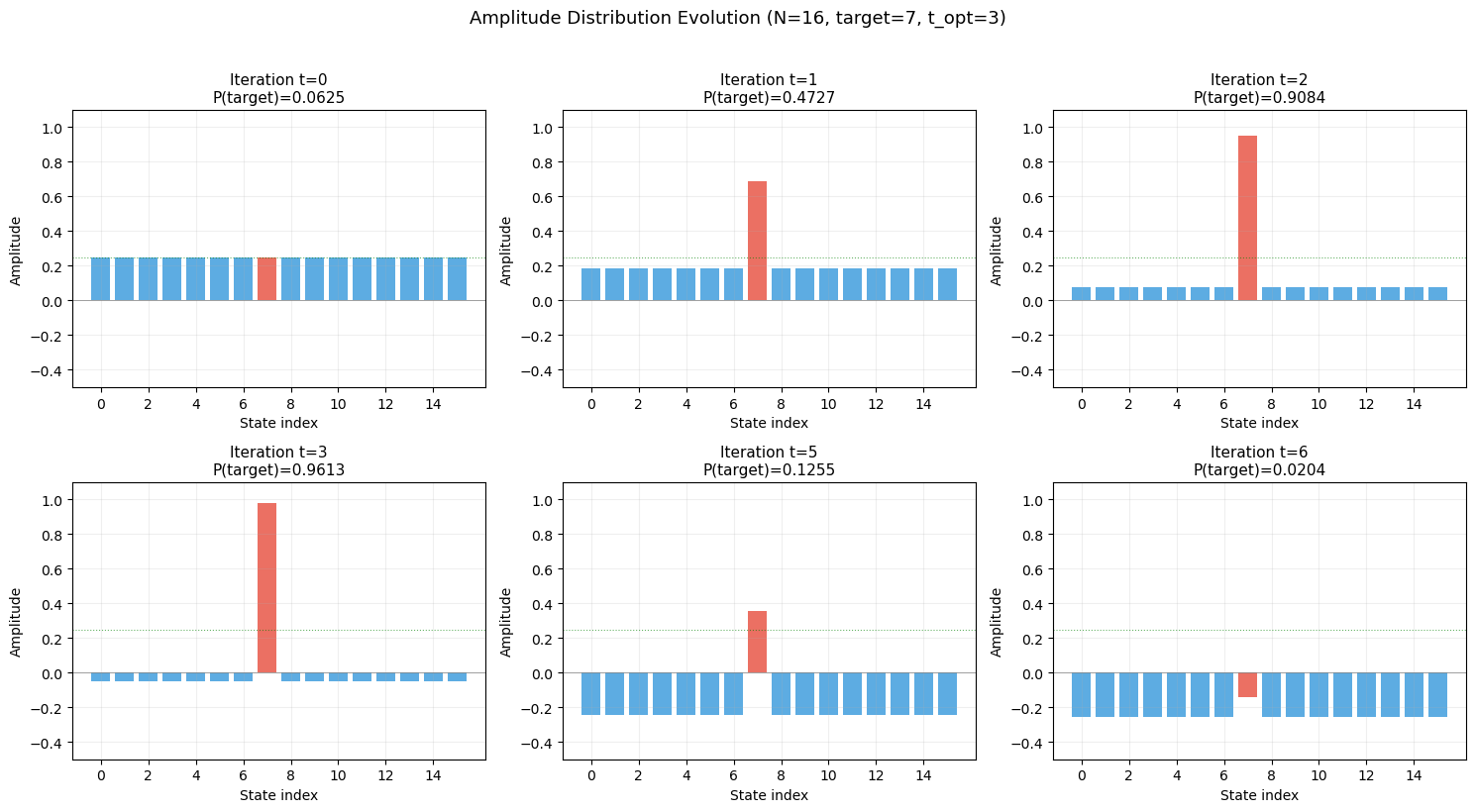
Observation
The amplitude bar charts reveal the “inversion about the mean” mechanism:
The oracle makes the target amplitude negative (below the mean).
The diffusion operator reflects all amplitudes about the mean, boosting the (now-negative) target amplitude to above the mean.
Each iteration increases the target amplitude by roughly \(2/\sqrt{N}\), while each non-target amplitude decreases slightly.
After \(t_{\text{opt}}\) iterations, nearly all probability mass is concentrated on the target state.
Experiment 6: Scaling Verification#
We verify that the optimal iteration count scales as \(\sqrt{N}\) by measuring the actual optimal iteration for each \(N\) and fitting.
Show code cell source
import numpy as np
import matplotlib.pyplot as plt
import math

n_qubits_range = range(2, 13)
measured_opt = []
predicted_opt = []
max_probs = []

for n_q in n_qubits_range:
    N = 2 ** n_q
    target = N // 3  # arbitrary target
    t_pred = int(np.floor(np.pi / 4 * np.sqrt(N)))

    # Sweep iterations to find actual optimum
    max_sweep = 2 * t_pred + 5
    history = grover_simulate_fast(n_q, target, n_iterations=max_sweep)
    probs = [h[target] ** 2 for h in history]

    best_t = np.argmax(probs)
    measured_opt.append(best_t)
    predicted_opt.append(t_pred)
    max_probs.append(probs[best_t])

n_vals = np.array([2 ** n for n in n_qubits_range])
sqrt_N = np.sqrt(n_vals.astype(float))

fig, (ax1, ax2) = plt.subplots(1, 2, figsize=(13, 5))

# Optimal iterations vs sqrt(N)
ax1.plot(sqrt_N, measured_opt, 'o', color='#e74c3c', markersize=8,
         label='Measured optimal $t$', zorder=3)
ax1.plot(sqrt_N, predicted_opt, 's', color='#3498db', markersize=6,
         label=r'Predicted $\lfloor\pi/4 * \sqrt{N}\rfloor$', zorder=3)

# Fit line
coeffs = np.polyfit(sqrt_N, measured_opt, 1)
fit_line = np.polyval(coeffs, sqrt_N)
ax1.plot(sqrt_N, fit_line, '--', color='gray', alpha=0.7,
         label=f'Linear fit: {float(coeffs[0]):.3f}$\\sqrt{{N}}$ + {float(coeffs[1]):.2f}')

ax1.set_xlabel(r'$\sqrt{N}$')
ax1.set_ylabel('Optimal iterations $t_{opt}$')
ax1.set_title(r'Scaling: $t_{opt}$ vs $\sqrt{N}$')
ax1.legend(fontsize=9)
ax1.grid(True, alpha=0.3)

# Maximum success probability vs N
ax2.plot(list(n_qubits_range), max_probs, 'o-', color='#2ecc71', markersize=6)
ax2.axhline(y=1.0, color='gray', linestyle=':', alpha=0.5)
ax2.set_xlabel('Number of qubits $n$')
ax2.set_ylabel('Maximum success probability')
ax2.set_title('Peak Success Probability vs. Problem Size')
ax2.set_ylim(0.85, 1.02)
ax2.grid(True, alpha=0.3)

plt.tight_layout()
plt.savefig('grover_scaling.png', dpi=150, bbox_inches='tight')
plt.show()

print(f'Fitted slope: {float(coeffs[0]):.4f} (expected: pi/4 = {float(np.pi/4):.4f})')
print(f'Fitted intercept: {float(coeffs[1]):.4f} (expected: ~0)')
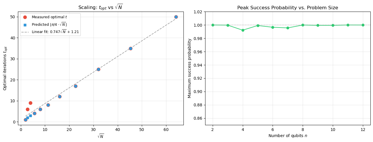
Fitted slope: 0.7471 (expected: pi/4 = 0.7854)
Fitted intercept: 1.2147 (expected: ~0)
39.6 Exercises#
Exercise 39.1 (Warm-up) Verify by hand that for \(N = 4\) (2 qubits) and target \(|11\rangle\), a single Grover iteration achieves success probability 1. Write out the state vector after the oracle and after the diffusion operator.
Hint
Start with \(|s\rangle = \frac{1}{2}(|00\rangle + |01\rangle + |10\rangle + |11\rangle)\). After the oracle: \(\frac{1}{2}(|00\rangle + |01\rangle + |10\rangle - |11\rangle)\). The mean amplitude is \(\frac{1}{4}(1/2 + 1/2 + 1/2 - 1/2) = 1/4\). After diffusion: each amplitude becomes \(2 \cdot 1/4 - \text{current}\). Check that only \(|11\rangle\) has nonzero amplitude.
Exercise 39.2 (Applied) Modify the simulation to handle multiple marked elements. If \(M\) out of \(N\) elements are marked, verify empirically that the optimal iteration count is \(\lfloor \frac{\pi}{4}\sqrt{N/M} \rfloor\) for \(M = 1, 2, 4, 8\) and \(N = 64\).
Hint
The oracle must flip the sign of all \(M\) marked states. The geometric analysis still applies but with \(\sin\theta = \sqrt{M/N}\) instead of \(\sin\theta = 1/\sqrt{N}\).
Exercise 39.3 (Analysis) Show analytically that the success probability after \(t\) iterations is exactly \(\sin^2((2t+1)\theta)\) where \(\theta = \arcsin(1/\sqrt{N})\). Use the 2D rotation picture.
Hint
Write the initial state as \(|s\rangle = \sin\theta|w\rangle + \cos\theta|w^\perp\rangle\). Show that one Grover iteration rotates by \(2\theta\) in the \(\{|w\rangle, |w^\perp\rangle\}\) plane. After \(t\) iterations the state is \(\sin((2t+1)\theta)|w\rangle + \cos((2t+1)\theta)|w^\perp\rangle\). The measurement probability is the coefficient of \(|w\rangle\) squared.
Exercise 39.4 (Theory) Prove that \(\Omega(\sqrt{N})\) quantum queries are necessary for unstructured search (BBBV lower bound). That is, show that Grover’s algorithm is optimal up to constant factors.
Hint
Use the polynomial method or the hybrid argument of Bennett, Bernstein, Brassard, and Vazirani (1997). The key insight is that each oracle query can change the state by at most \(O(1/\sqrt{N})\) in \(\ell_2\) norm, so reaching a state that distinguishes the target from “no target” requires \(\Omega(\sqrt{N})\) queries.
Exercise 39.5 (Challenge) Implement a simulation of Grover’s algorithm applied to AES key search for a toy version: use a 16-bit block and 16-bit key with a 2-round SPN. Given one known plaintext-ciphertext pair, implement the oracle that checks whether a candidate key produces the correct ciphertext, and estimate the number of Grover iterations needed.
Hint
The oracle \(f(k) = 1\) if and only if \(\text{Encrypt}(k, P) = C\). For a 16-bit key, \(N = 2^{16} = 65536\) and \(t_{\text{opt}} \approx 201\) iterations. You can simulate this classically but it will require storing a \(2^{16}\)-dimensional amplitude vector.
39.7 Summary#
Concept |
Key Point |
|---|---|
Grover’s algorithm |
Quadratic speedup for unstructured search: \(O(\sqrt{N})\) vs \(O(N)\) |
Oracle \(U_f\) |
Phase flip: \(U_f\vert x\rangle = (-1)^{f(x)}\vert x\rangle\), a reflection |
Diffusion operator \(D\) |
Inversion about the mean: \(D = 2\vert s\rangle\langle s\vert - I\) |
Optimal iterations |
\(t_{\text{opt}} = \lfloor \pi/4 \cdot \sqrt{N} \rfloor\) |
Geometric picture |
Rotation by \(2\theta\) per iteration in 2D subspace |
Multiple solutions |
\(M\) solutions: optimal iterations \(\lfloor \pi/4 \cdot \sqrt{N/M} \rfloor\) |
AES impact |
\(k\)-bit key \(\to\) \(k/2\)-bit effective security; AES-256 recommended |
Optimality |
BBBV lower bound: \(\Omega(\sqrt{N})\) queries are necessary |
Tip
Grover’s algorithm has a quadratic speedup, compared to Shor’s exponential speedup for factoring. This is why post-quantum cryptography focuses primarily on replacing public-key primitives (RSA, ECC) rather than symmetric ciphers – doubling the key length of AES suffices to restore security against Grover.
References#
Grover, L. K. (1996). A Fast Quantum Mechanical Algorithm for Database Search. Proceedings of the 28th Annual ACM Symposium on Theory of Computing (STOC), 212–219.
Bennett, C. H., Bernstein, E., Brassard, G., and Vazirani, U. (1997). Strengths and Weaknesses of Quantum Computing. SIAM Journal on Computing, 26(5), 1510–1523.
Boyer, M., Brassard, G., H\u00f8yer, P., and Tapp, A. (1998). Tight Bounds on Quantum Searching. Fortschritte der Physik, 46(4–5), 493–505.
Nielsen, M. A. and Chuang, I. L. (2010). Quantum Computation and Quantum Information. 10th Anniversary Edition, Cambridge University Press.
NIST (2016). Report on Post-Quantum Cryptography. NISTIR 8105.