
Chapter 16: Foundations of Linear Cryptanalysis#
16.1 Historical Context: Matsui’s Breakthrough#
In 1993, at the EUROCRYPT conference in Lofthus, Norway, Mitsuru Matsui presented a paper that would fundamentally change the landscape of block cipher analysis. Titled “Linear Cryptanalysis Method for DES Cipher,” this work introduced a novel attack paradigm that exploited linear statistical relationships between plaintext bits, ciphertext bits, and key bits. Within a year, Matsui refined the method and demonstrated a practical key-recovery attack on the full 16-round Data Encryption Standard (DES) using approximately \(2^{43}\) known plaintext-ciphertext pairs – the first publicly known attack on full DES that was faster than brute-force search over the \(2^{56}\)-bit key space.
The significance of this achievement cannot be overstated. DES had been the de facto standard for symmetric encryption since 1977. Despite decades of intensive cryptanalytic scrutiny, no public attack had broken the full cipher faster than exhaustive key search. Differential cryptanalysis, introduced by Biham and Shamir in 1990, required \(2^{47}\) chosen plaintexts – a chosen-plaintext attack that was theoretically powerful but practically difficult to mount. Matsui’s linear cryptanalysis, by contrast, required only known plaintexts, making it significantly more practical in real-world scenarios where an attacker might passively collect plaintext-ciphertext pairs.
“The purpose of this paper is to present a new method, called linear cryptanalysis, for cryptanalysis of DES cipher and to show that DES is breakable with \(2^{43}\) known plaintext-ciphertext pairs.”
– Mitsuru Matsui, Linear Cryptanalysis Method for DES Cipher, EUROCRYPT 1993
The core idea behind linear cryptanalysis is deceptively simple. Consider a block cipher as a complex nonlinear function mapping plaintext \(P\) and key \(K\) to ciphertext \(C\). Although this function is designed to be highly nonlinear (to resist algebraic attacks), it is never perfectly nonlinear. For certain choices of bit positions – specified by input masks \(\alpha\) and output masks \(\beta\) – the XOR of selected plaintext bits and selected ciphertext bits correlates with the XOR of certain key bits:
This equation holds not with certainty, but with probability \(p = \frac{1}{2} + \varepsilon\), where \(\varepsilon\) is the bias. If \(\varepsilon\) is non-negligible, collecting enough known plaintext-ciphertext pairs allows the attacker to determine the value of the key-bit XOR with high confidence. By constructing multiple such linear approximations and combining them, the attacker can recover the full key.
Important
Linear cryptanalysis is a known-plaintext attack. Unlike differential cryptanalysis, which requires the attacker to choose specific plaintext pairs, linear cryptanalysis only requires the attacker to observe plaintext-ciphertext pairs encrypted under the same key. This makes it significantly more practical in many real-world scenarios.
Matsui’s work had profound consequences for cipher design. Every modern block cipher – including AES (Rijndael), Serpent, Twofish, and Camellia – is now explicitly designed to resist linear cryptanalysis. The maximum bias of the S-box linear approximation table became a primary design criterion, and the wide trail strategy used in AES was specifically engineered to ensure that any linear approximation spanning multiple rounds accumulates negligibly small bias.
16.2 Formal Definitions#
We now develop the mathematical foundations of linear cryptanalysis with full rigor. Throughout this section, we work over \(\mathbb{F}_2 = \{0, 1\}\), the field with two elements, where addition is XOR (\(\oplus\)).
Boolean Functions and Inner Products#
For a vector \(x = (x_1, x_2, \ldots, x_n) \in \mathbb{F}_2^n\) and a mask \(\alpha = (\alpha_1, \alpha_2, \ldots, \alpha_n) \in \mathbb{F}_2^n\), the inner product is:
This selects and XORs exactly those bits of \(x\) where the corresponding bit of \(\alpha\) is 1.
Definition 16.1 (Linear Approximation of a Boolean Function)
Let \(S: \mathbb{F}_2^n \to \mathbb{F}_2^m\) be a vectorial Boolean function (such as an S-box). A linear approximation of \(S\) with input mask \(\alpha \in \mathbb{F}_2^n\) and output mask \(\beta \in \mathbb{F}_2^m\) is the Boolean equation:
or equivalently:
The probability of this approximation is:
For a random function, we would expect \(p(\alpha, \beta) = 1/2\) for all non-trivial masks (i.e., \((\alpha, \beta) \neq (0, 0)\)). The degree to which an S-box deviates from this ideal is captured by the bias.
Definition 16.2 (Bias)
The bias of a linear approximation \((\alpha, \beta)\) for a function \(S\) is:
Equivalently, if we define the random variable \(X = \langle \alpha, x \rangle \oplus \langle \beta, S(x) \rangle\), then:
The bias satisfies \(-\frac{1}{2} \leq \varepsilon \leq \frac{1}{2}\), with \(\varepsilon = 0\) indicating a perfectly balanced (ideal) approximation.
Definition 16.3 (Linear Approximation Table)
The Linear Approximation Table (LAT) of an S-box \(S: \mathbb{F}_2^n \to \mathbb{F}_2^m\) is the \((2^n) \times (2^m)\) matrix \(\Lambda\) where:
Each entry \(\Lambda[\alpha][\beta]\) is related to the bias by \(\varepsilon(\alpha, \beta) = \Lambda[\alpha][\beta] / 2^n\).
The LAT has the following properties:
\(\Lambda[0][0] = 2^{n-1}\) (the trivial approximation always holds for all inputs, so the count is \(2^n\) and the entry is \(2^n - 2^{n-1} = 2^{n-1}\)).
\(\Lambda[\alpha][0] = 0\) for \(\alpha \neq 0\) (any non-trivial input mask with trivial output mask is balanced for a permutation).
All entries are integers with the same parity.
16.3 The Piling-Up Lemma#
The piling-up lemma is the theoretical engine that powers linear cryptanalysis. It tells us how to combine biases of individual round approximations to estimate the bias of a multi-round linear approximation.
Theorem 16.1 (Piling-Up Lemma, Matsui 1993)
Let \(X_1, X_2, \ldots, X_n\) be independent binary random variables with biases \(\varepsilon_i = \Pr[X_i = 0] - 1/2\) for \(i = 1, \ldots, n\). Then the bias of their XOR is:
That is, if \(Y = X_1 \oplus X_2 \oplus \cdots \oplus X_n\), then:
Proof of the Piling-Up Lemma
Base case (\(n = 2\)). Let \(X_1, X_2\) be independent binary random variables with \(\Pr[X_i = 0] = 1/2 + \varepsilon_i\), so \(\Pr[X_i = 1] = 1/2 - \varepsilon_i\).
We compute \(\Pr[X_1 \oplus X_2 = 0]\). Since \(X_1 \oplus X_2 = 0\) iff both are 0 or both are 1:
(by independence). Substituting:
Expanding the first product:
Expanding the second product:
Adding:
So the bias of \(X_1 \oplus X_2\) is \(2\varepsilon_1\varepsilon_2 = 2^{2-1}\varepsilon_1\varepsilon_2\). This confirms the formula for \(n = 2\).
Inductive step. Assume the result holds for \(n-1\) variables: the bias of \(Y_{n-1} = X_1 \oplus \cdots \oplus X_{n-1}\) is \(\varepsilon_{Y_{n-1}} = 2^{n-2}\prod_{i=1}^{n-1}\varepsilon_i\).
Now \(Y_n = Y_{n-1} \oplus X_n\). Since \(Y_{n-1}\) depends only on \(X_1, \ldots, X_{n-1}\) and \(X_n\) is independent of all of these, \(Y_{n-1}\) and \(X_n\) are independent. Applying the base case:
This completes the induction. \(\square\)
Warning
The independence assumption is crucial. The piling-up lemma assumes that the random variables \(X_1, \ldots, X_n\) are independent. In the context of a block cipher, these correspond to the linear approximations of individual S-boxes or individual rounds. In practice, the approximations are not perfectly independent because they share intermediate state bits. However, the heuristic assumption of independence (sometimes called the linear hull hypothesis) works remarkably well in practice, and the piling-up lemma gives good predictions for the bias of multi-round approximations.
16.4 Python Implementation: The LinearAnalyzer Class#
We now implement the core tools for linear cryptanalysis. The LinearAnalyzer class computes the full linear approximation table (LAT) of any S-box, extracts biases, and identifies the most exploitable linear approximations.
import numpy as np
import matplotlib.pyplot as plt
class LinearAnalyzer:
"""
Linear cryptanalysis toolkit for S-box analysis.
Given an S-box S: F_2^n -> F_2^m (represented as a lookup table),
this class computes the Linear Approximation Table (LAT), extracts
biases for specific mask pairs, and identifies the strongest linear
approximations.
Parameters
----------
sbox : list or np.ndarray
The S-box lookup table. sbox[x] = S(x).
For a 4-bit S-box, this is a list of 16 integers in {0,...,15}.
Attributes
----------
n_input : int
Number of input bits (log2 of input size).
n_output : int
Number of output bits (log2 of max output value + 1).
lat : np.ndarray
The Linear Approximation Table (counts minus 2^{n-1}).
"""
def __init__(self, sbox):
self.sbox = np.array(sbox, dtype=int)
self.size = len(sbox)
self.n_input = int(np.log2(self.size))
self.n_output = int(np.log2(max(sbox) + 1))
# Verify power-of-2 size
assert self.size == 2**self.n_input, "S-box size must be a power of 2"
self.lat = self.compute_lat(self.sbox)
@staticmethod
def _inner_product(mask, value):
"""Compute the inner product <mask, value> over F_2."""
# XOR of bits where mask is 1 = parity of (mask AND value)
return bin(mask & value).count('1') % 2
@staticmethod
def compute_lat(sbox):
"""
Compute the Linear Approximation Table of an S-box.
For input mask alpha and output mask beta, compute:
LAT[alpha][beta] = #{x : <alpha,x> = <beta,S(x)>} - 2^{n-1}
Parameters
----------
sbox : array-like
The S-box lookup table.
Returns
-------
lat : np.ndarray
The LAT matrix with shape (2^n, 2^m).
"""
sbox = np.array(sbox, dtype=int)
n = len(sbox)
n_bits_in = int(np.log2(n))
n_bits_out = int(np.log2(max(sbox) + 1))
n_out = 2**n_bits_out
half = n // 2
lat = np.zeros((n, n_out), dtype=int)
for alpha in range(n):
for beta in range(n_out):
count = 0
for x in range(n):
# Compute <alpha, x> XOR <beta, S(x)>
lhs = bin(alpha & x).count('1') % 2
rhs = bin(beta & sbox[x]).count('1') % 2
if lhs == rhs:
count += 1
lat[alpha][beta] = count - half
return lat
def bias(self, input_mask, output_mask):
"""
Compute the bias for a given (input_mask, output_mask) pair.
Parameters
----------
input_mask : int
The input mask alpha.
output_mask : int
The output mask beta.
Returns
-------
float
The bias epsilon = LAT[alpha][beta] / 2^n.
"""
return self.lat[input_mask][output_mask] / self.size
def best_approximations(self, n=10):
"""
Find the top-n linear approximations with largest absolute bias.
Parameters
----------
n : int
Number of top approximations to return.
Returns
-------
list of tuples
Each tuple is (input_mask, output_mask, bias_value).
Sorted by |bias| in descending order.
Excludes the trivial approximation (0, 0).
"""
results = []
n_out = self.lat.shape[1]
for alpha in range(self.size):
for beta in range(n_out):
if alpha == 0 and beta == 0:
continue # skip trivial
b = self.lat[alpha][beta] / self.size
results.append((alpha, beta, b))
# Sort by absolute bias, descending
results.sort(key=lambda t: abs(t[2]), reverse=True)
return results[:n]
def print_lat(self):
"""Print the LAT in a formatted table."""
n_out = self.lat.shape[1]
header = " " + "".join(f"{b:4X}" for b in range(n_out))
print(header)
print(" " + "-" * (4 * n_out + 1))
for alpha in range(self.size):
row = f"{alpha:2X} | " + "".join(f"{int(self.lat[alpha][b]):4d}" for b in range(n_out))
print(row)
# === Define the Heys S-box (from Heys' tutorial) ===
HEYS_SBOX = [0xE, 0x4, 0xD, 0x1, 0x2, 0xF, 0xB, 0x8,
0x3, 0xA, 0x6, 0xC, 0x5, 0x9, 0x0, 0x7]
print("Heys S-box:", [hex(x) for x in HEYS_SBOX])
print()
# Create the analyzer
analyzer = LinearAnalyzer(HEYS_SBOX)
print(f"S-box size: {analyzer.size} ({analyzer.n_input}-bit input, {analyzer.n_output}-bit output)")
print()
# Print the full LAT
print("Linear Approximation Table (LAT):")
print("Rows = input mask (alpha), Columns = output mask (beta)")
print("Entries = count - 2^{n-1} (so bias = entry / 2^n)")
print()
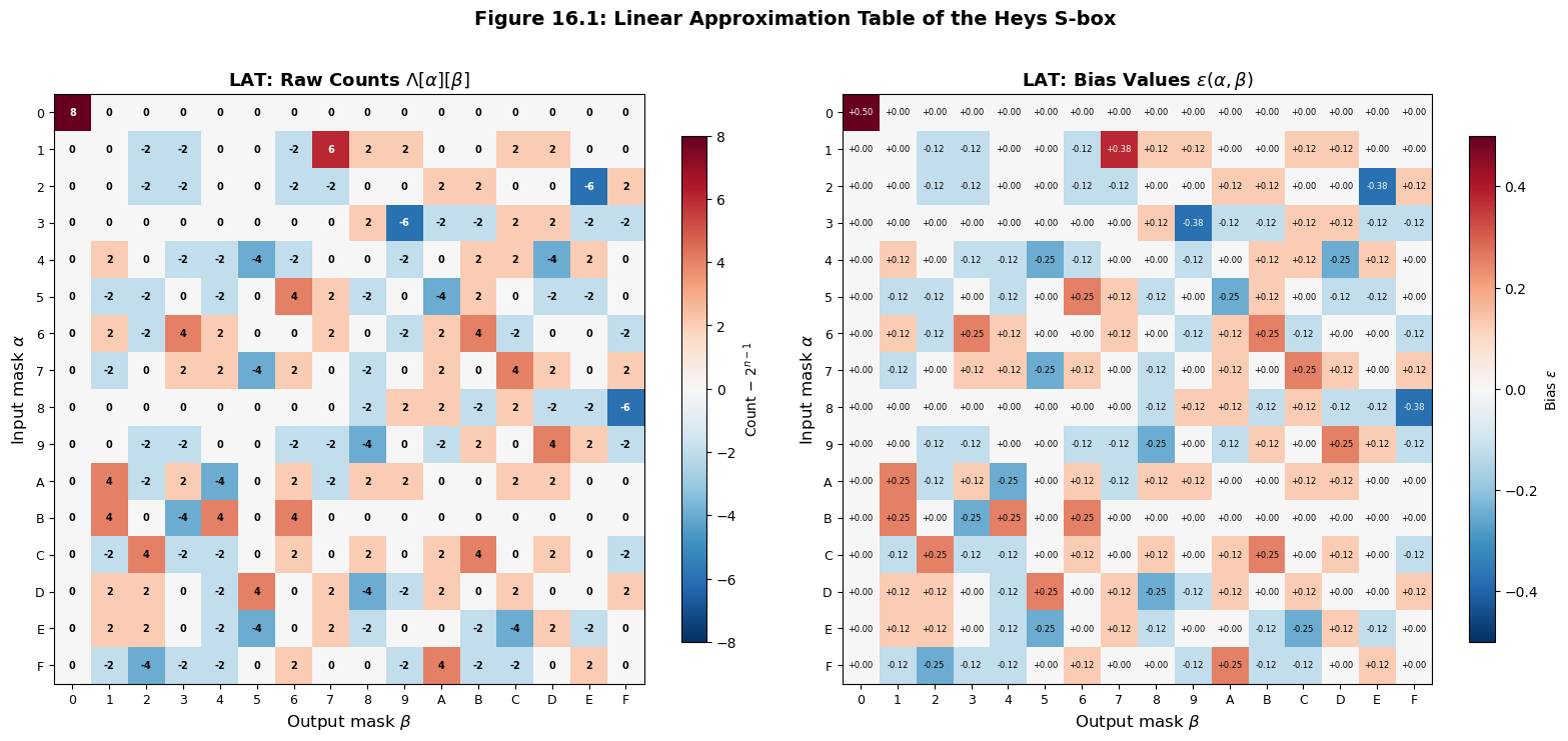
analyzer.print_lat()
Heys S-box: ['0xe', '0x4', '0xd', '0x1', '0x2', '0xf', '0xb', '0x8', '0x3', '0xa', '0x6', '0xc', '0x5', '0x9', '0x0', '0x7']

S-box size: 16 (4-bit input, 4-bit output)

Linear Approximation Table (LAT):
Rows = input mask (alpha), Columns = output mask (beta)
Entries = count - 2^{n-1} (so bias = entry / 2^n)

        0   1   2   3   4   5   6   7   8   9   A   B   C   D   E   F
    -----------------------------------------------------------------
 0 |    8   0   0   0   0   0   0   0   0   0   0   0   0   0   0   0
 1 |    0   0  -2  -2   0   0  -2   6   2   2   0   0   2   2   0   0
 2 |    0   0  -2  -2   0   0  -2  -2   0   0   2   2   0   0  -6   2
 3 |    0   0   0   0   0   0   0   0   2  -6  -2  -2   2   2  -2  -2
 4 |    0   2   0  -2  -2  -4  -2   0   0  -2   0   2   2  -4   2   0
 5 |    0  -2  -2   0  -2   0   4   2  -2   0  -4   2   0  -2  -2   0
 6 |    0   2  -2   4   2   0   0   2   0  -2   2   4  -2   0   0  -2
 7 |    0  -2   0   2   2  -4   2   0  -2   0   2   0   4   2   0   2
 8 |    0   0   0   0   0   0   0   0  -2   2   2  -2   2  -2  -2  -6
 9 |    0   0  -2  -2   0   0  -2  -2  -4   0  -2   2   0   4   2  -2
 A |    0   4  -2   2  -4   0   2  -2   2   2   0   0   2   2   0   0
 B |    0   4   0  -4   4   0   4   0   0   0   0   0   0   0   0   0
 C |    0  -2   4  -2  -2   0   2   0   2   0   2   4   0   2   0  -2
 D |    0   2   2   0  -2   4   0   2  -4  -2   2   0   2   0   0   2
 E |    0   2   2   0  -2  -4   0   2  -2   0   0  -2  -4   2  -2   0
 F |    0  -2  -4  -2  -2   0   2   0   0  -2   4  -2  -2   0   2   0
Identifying the Strongest Approximations#
The most useful linear approximations for an attacker are those with the largest absolute bias. Let us extract and examine them.
import numpy as np
import matplotlib.pyplot as plt

# Recreate the analyzer
HEYS_SBOX = [0xE, 0x4, 0xD, 0x1, 0x2, 0xF, 0xB, 0x8,
             0x3, 0xA, 0x6, 0xC, 0x5, 0x9, 0x0, 0x7]

# Redefine helper for standalone execution
def compute_lat(sbox):
    sbox = np.array(sbox, dtype=int)
    n = len(sbox)
    n_out = 2**int(np.log2(max(sbox) + 1))
    half = n // 2
    lat = np.zeros((n, n_out), dtype=int)
    for alpha in range(n):
        for beta in range(n_out):
            count = 0
            for x in range(n):
                lhs = bin(alpha & x).count('1') % 2
                rhs = bin(beta & sbox[x]).count('1') % 2
                if lhs == rhs:
                    count += 1
            lat[alpha][beta] = count - half
    return lat

lat = compute_lat(HEYS_SBOX)
n = len(HEYS_SBOX)

# Find best approximations
results = []
for alpha in range(n):
    for beta in range(n):
        if alpha == 0 and beta == 0:
            continue
        bias = lat[alpha][beta] / n
        results.append((alpha, beta, bias))

results.sort(key=lambda t: abs(t[2]), reverse=True)

print("Top 15 Linear Approximations for Heys S-box")
print("=" * 62)
print(f"{'Rank':>4s}  {'alpha':>6s}  {'beta':>6s}  {'LAT entry':>10s}  {'Bias':>10s}  {'|Bias|':>8s}")
print("-" * 62)
for rank, (a, b, bias) in enumerate(results[:15], 1):
    print(f"{int(rank):4d}  0x{a:01X} ({a:04b})  0x{b:01X} ({b:04b})  {int(lat[a][b]):10d}  {float(bias):10.4f}  {float(abs(bias)):8.4f}")

print()
print("Key observations:")
max_abs_bias = max(abs(r[2]) for r in results)
count_max = sum(1 for r in results if abs(r[2]) == max_abs_bias)
print(f"  - Maximum absolute bias: {float(max_abs_bias):.4f}")
print(f"  - Number of approximations achieving max |bias|: {count_max}")
print(f"  - Bias = {float(max_abs_bias):.4f} means probability = {float(0.5 + max_abs_bias):.4f}")
print(f"  - These are the most exploitable approximations for linear cryptanalysis")
Top 15 Linear Approximations for Heys S-box
==============================================================
Rank   alpha    beta   LAT entry        Bias    |Bias|
--------------------------------------------------------------
   1  0x1 (0001)  0x7 (0111)           6      0.3750    0.3750
   2  0x2 (0010)  0xE (1110)          -6     -0.3750    0.3750
   3  0x3 (0011)  0x9 (1001)          -6     -0.3750    0.3750
   4  0x8 (1000)  0xF (1111)          -6     -0.3750    0.3750
   5  0x4 (0100)  0x5 (0101)          -4     -0.2500    0.2500
   6  0x4 (0100)  0xD (1101)          -4     -0.2500    0.2500
   7  0x5 (0101)  0x6 (0110)           4      0.2500    0.2500
   8  0x5 (0101)  0xA (1010)          -4     -0.2500    0.2500
   9  0x6 (0110)  0x3 (0011)           4      0.2500    0.2500
  10  0x6 (0110)  0xB (1011)           4      0.2500    0.2500
  11  0x7 (0111)  0x5 (0101)          -4     -0.2500    0.2500
  12  0x7 (0111)  0xC (1100)           4      0.2500    0.2500
  13  0x9 (1001)  0x8 (1000)          -4     -0.2500    0.2500
  14  0x9 (1001)  0xD (1101)           4      0.2500    0.2500
  15  0xA (1010)  0x1 (0001)           4      0.2500    0.2500

Key observations:
  - Maximum absolute bias: 0.3750
  - Number of approximations achieving max |bias|: 4
  - Bias = 0.3750 means probability = 0.8750
  - These are the most exploitable approximations for linear cryptanalysis
16.5 Visualizing the Linear Approximation Table#
The LAT reveals the linear structure hidden within a nonlinear S-box. A heatmap visualization makes it easy to spot strong approximations (dark red or dark blue) and assess the overall linearity profile.
Show code cell source
import numpy as np
import matplotlib.pyplot as plt

HEYS_SBOX = [0xE, 0x4, 0xD, 0x1, 0x2, 0xF, 0xB, 0x8,
             0x3, 0xA, 0x6, 0xC, 0x5, 0x9, 0x0, 0x7]

def compute_lat(sbox):
    sbox = np.array(sbox, dtype=int)
    n = len(sbox)
    n_out = 2**int(np.log2(max(sbox) + 1))
    half = n // 2
    lat = np.zeros((n, n_out), dtype=int)
    for alpha in range(n):
        for beta in range(n_out):
            count = 0
            for x in range(n):
                lhs = bin(alpha & x).count('1') % 2
                rhs = bin(beta & sbox[x]).count('1') % 2
                if lhs == rhs:
                    count += 1
            lat[alpha][beta] = count - half
    return lat

lat = compute_lat(HEYS_SBOX)
n = len(HEYS_SBOX)

# Convert to bias values
bias_table = lat / n

fig, axes = plt.subplots(1, 2, figsize=(16, 7))

# Left: Raw LAT counts
im1 = axes[0].imshow(lat, cmap='RdBu_r', aspect='equal', interpolation='nearest',
                      vmin=-8, vmax=8)
axes[0].set_title('LAT: Raw Counts $\\Lambda[\\alpha][\\beta]$', fontsize=13, fontweight='bold')
axes[0].set_xlabel('Output mask $\\beta$', fontsize=12)
axes[0].set_ylabel('Input mask $\\alpha$', fontsize=12)
axes[0].set_xticks(range(16))
axes[0].set_yticks(range(16))
axes[0].set_xticklabels([f'{i:X}' for i in range(16)], fontsize=9)
axes[0].set_yticklabels([f'{i:X}' for i in range(16)], fontsize=9)
# Add text annotations
for i in range(16):
    for j in range(16):
        color = 'white' if abs(lat[i][j]) >= 5 else 'black'
        axes[0].text(j, i, f'{int(lat[i][j]):d}', ha='center', va='center',
                     fontsize=7, color=color, fontweight='bold')
fig.colorbar(im1, ax=axes[0], shrink=0.8, label='Count $-$ $2^{n-1}$')

# Right: Bias values
im2 = axes[1].imshow(bias_table, cmap='RdBu_r', aspect='equal', interpolation='nearest',
                      vmin=-0.5, vmax=0.5)
axes[1].set_title('LAT: Bias Values $\\varepsilon(\\alpha, \\beta)$', fontsize=13, fontweight='bold')
axes[1].set_xlabel('Output mask $\\beta$', fontsize=12)
axes[1].set_ylabel('Input mask $\\alpha$', fontsize=12)
axes[1].set_xticks(range(16))
axes[1].set_yticks(range(16))
axes[1].set_xticklabels([f'{i:X}' for i in range(16)], fontsize=9)
axes[1].set_yticklabels([f'{i:X}' for i in range(16)], fontsize=9)
for i in range(16):
    for j in range(16):
        val = bias_table[i][j]
        color = 'white' if abs(val) >= 0.3 else 'black'
        axes[1].text(j, i, f'{val:+.2f}', ha='center', va='center',
                     fontsize=6, color=color)
fig.colorbar(im2, ax=axes[1], shrink=0.8, label='Bias $\\varepsilon$')

fig.suptitle('Figure 16.1: Linear Approximation Table of the Heys S-box',
             fontsize=14, fontweight='bold', y=1.02)

plt.tight_layout()
plt.savefig('fig_16_1_heys_lat_heatmap.png', dpi=150, bbox_inches='tight', facecolor='white')
plt.show()
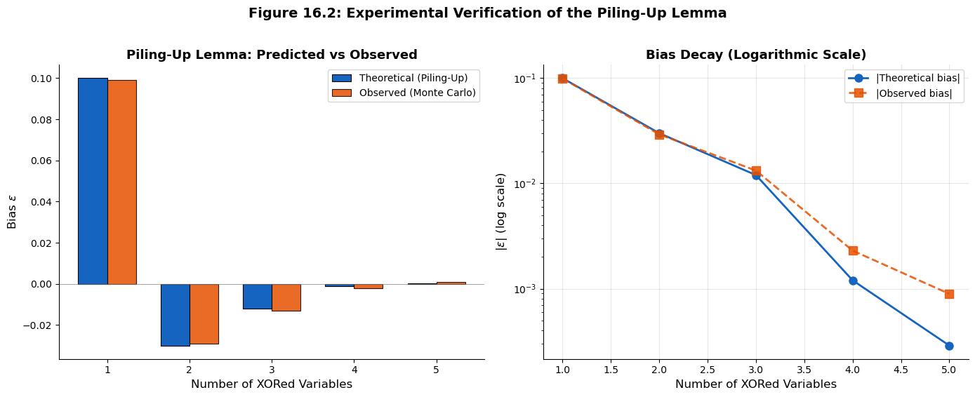
16.6 Experimental Verification of the Piling-Up Lemma#
The piling-up lemma predicts how biases compose when independent random variables are XORed. Let us verify this experimentally by generating biased random variables and comparing the observed bias of their XOR against the theoretical prediction.
Show code cell source
import numpy as np
import matplotlib.pyplot as plt

np.random.seed(42)

def generate_biased_bits(n_samples, bias):
    """
    Generate n_samples binary random variables with given bias.
    P(X=0) = 0.5 + bias, P(X=1) = 0.5 - bias
    """
    prob_zero = 0.5 + bias
    return (np.random.random(n_samples) >= prob_zero).astype(int)

def observed_bias(bits):
    """Compute observed bias: P(X=0) - 0.5"""
    return np.mean(bits == 0) - 0.5

# Experiment: XOR of n biased variables
n_samples = 500_000
individual_biases = [0.1, -0.15, 0.2, 0.05, -0.12]

print("Piling-Up Lemma Verification")
print("=" * 70)
print(f"Number of samples: {n_samples:,}")
print()

# Generate individual biased bits
bits_list = [generate_biased_bits(n_samples, eps) for eps in individual_biases]

# Verify individual biases
print("Individual variable biases:")
for i, (eps_true, bits) in enumerate(zip(individual_biases, bits_list)):
    eps_obs = observed_bias(bits)
    print(f"  X_{i+1}: true bias = {eps_true:+.4f}, observed bias = {eps_obs:+.4f}")
print()

# XOR progressively more variables and check
xor_bits = bits_list[0].copy()
theoretical_biases = [individual_biases[0]]
observed_biases = [observed_bias(xor_bits)]
n_vars_list = [1]

print("Progressive XOR results:")
print(f"{'n vars':>7s}  {'Theoretical bias':>18s}  {'Observed bias':>16s}  {'Relative error':>16s}")
print("-" * 65)

# For n=1, the theoretical bias is just eps_1
theo = individual_biases[0]
obs = observed_bias(xor_bits)
rel_err = abs(theo - obs) / abs(theo) if theo != 0 else 0
print(f"{int(1):7d}  {theo:+18.8f}  {obs:+16.8f}  {float(rel_err):16.4%}")

for k in range(1, len(individual_biases)):
    xor_bits = xor_bits ^ bits_list[k]

    # Piling-up lemma: bias = 2^{n-1} * product of individual biases
    n_combined = k + 1
    theo = (2**(n_combined - 1)) * np.prod(individual_biases[:n_combined])
    obs = observed_bias(xor_bits)
    rel_err = abs(theo - obs) / abs(theo) if theo != 0 else 0

    theoretical_biases.append(theo)
    observed_biases.append(obs)
    n_vars_list.append(n_combined)

    print(f"{int(n_combined):7d}  {theo:+18.8f}  {obs:+16.8f}  {float(rel_err):16.4%}")

# Plot
fig, axes = plt.subplots(1, 2, figsize=(14, 5.5))

# Left: Theoretical vs Observed bias
x_pos = np.arange(len(n_vars_list))
width = 0.35
bars1 = axes[0].bar(x_pos - width/2, theoretical_biases, width, label='Theoretical (Piling-Up)',
                     color='#1565C0', edgecolor='black', linewidth=0.8)
bars2 = axes[0].bar(x_pos + width/2, observed_biases, width, label='Observed (Monte Carlo)',
                     color='#E65100', edgecolor='black', linewidth=0.8, alpha=0.85)
axes[0].set_xlabel('Number of XORed Variables', fontsize=12)
axes[0].set_ylabel('Bias $\\varepsilon$', fontsize=12)
axes[0].set_title('Piling-Up Lemma: Predicted vs Observed', fontsize=13, fontweight='bold')
axes[0].set_xticks(x_pos)
axes[0].set_xticklabels(n_vars_list)
axes[0].legend(fontsize=10)
axes[0].axhline(y=0, color='gray', linestyle='-', linewidth=0.5)
axes[0].spines['top'].set_visible(False)
axes[0].spines['right'].set_visible(False)

# Right: |Bias| on log scale to show exponential decay
abs_theo = [abs(b) for b in theoretical_biases]
abs_obs = [abs(b) for b in observed_biases]
axes[1].semilogy(n_vars_list, abs_theo, 'o-', color='#1565C0', linewidth=2,
                  markersize=8, label='|Theoretical bias|')
axes[1].semilogy(n_vars_list, abs_obs, 's--', color='#E65100', linewidth=2,
                  markersize=8, label='|Observed bias|', alpha=0.85)
axes[1].set_xlabel('Number of XORed Variables', fontsize=12)
axes[1].set_ylabel('$|\\varepsilon|$ (log scale)', fontsize=12)
axes[1].set_title('Bias Decay (Logarithmic Scale)', fontsize=13, fontweight='bold')
axes[1].legend(fontsize=10)
axes[1].grid(True, alpha=0.3)
axes[1].spines['top'].set_visible(False)
axes[1].spines['right'].set_visible(False)

fig.suptitle('Figure 16.2: Experimental Verification of the Piling-Up Lemma',
             fontsize=14, fontweight='bold', y=1.02)

plt.tight_layout()
plt.savefig('fig_16_2_piling_up_verification.png', dpi=150, bbox_inches='tight', facecolor='white')
plt.show()
Piling-Up Lemma Verification
======================================================================
Number of samples: 500,000

Individual variable biases:
  X_1: true bias = +0.1000, observed bias = +0.0992
  X_2: true bias = -0.1500, observed bias = -0.1504
  X_3: true bias = +0.2000, observed bias = +0.2017
  X_4: true bias = +0.0500, observed bias = +0.0509
  X_5: true bias = -0.1200, observed bias = -0.1199

Progressive XOR results:
 n vars    Theoretical bias     Observed bias    Relative error
-----------------------------------------------------------------
      1         +0.10000000       +0.09923600           0.7640%
      2         -0.03000000       -0.02925000           2.5000%
      3         -0.01200000       -0.01323800          10.3167%
      4         -0.00120000       -0.00230000          91.6667%
      5         +0.00028800       +0.00089200         209.7222%
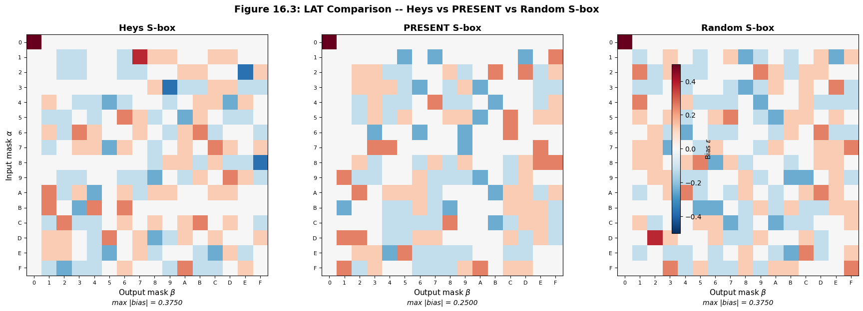
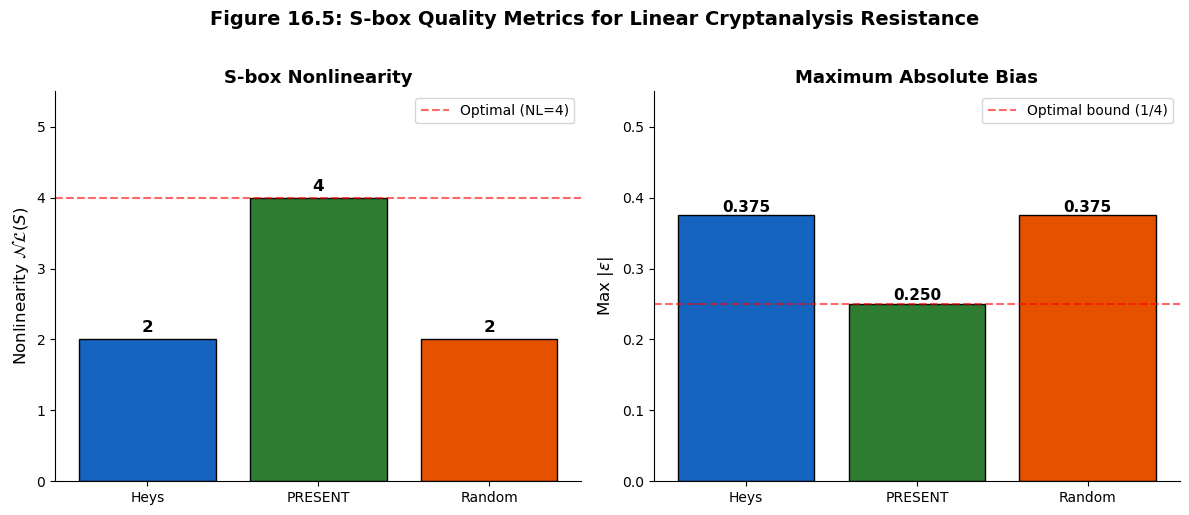
16.7 Comparing S-box Linearity: Heys vs PRESENT vs Random#
A well-designed S-box should minimize the maximum absolute bias in its LAT (excluding the trivial entry). Let us compare three S-boxes:
Heys S-box – the 4-bit educational S-box from Heys’ tutorial
PRESENT S-box – a well-designed 4-bit S-box from the PRESENT lightweight cipher, which is known to achieve optimal nonlinearity
Random permutation – a randomly generated 4-bit permutation
For an ideal \(n\)-bit S-box, the maximum absolute bias is bounded below by \(2^{-n/2}\) (the “bent function” bound for \(n\) even). For \(n = 4\), this gives \(|\varepsilon|_{\max} \geq 1/4\), so no 4-bit S-box can achieve maximum bias below \(1/4\).
Show code cell source
import numpy as np
import matplotlib.pyplot as plt

def compute_lat(sbox):
    sbox = np.array(sbox, dtype=int)
    n = len(sbox)
    n_out = 2**int(np.log2(max(sbox) + 1))
    half = n // 2
    lat = np.zeros((n, n_out), dtype=int)
    for alpha in range(n):
        for beta in range(n_out):
            count = 0
            for x in range(n):
                lhs = bin(alpha & x).count('1') % 2
                rhs = bin(beta & sbox[x]).count('1') % 2
                if lhs == rhs:
                    count += 1
            lat[alpha][beta] = count - half
    return lat

def max_absolute_bias(lat, n):
    """Max absolute bias excluding trivial (0,0) entry."""
    best = 0
    for a in range(lat.shape[0]):
        for b in range(lat.shape[1]):
            if a == 0 and b == 0:
                continue
            best = max(best, abs(lat[a][b]))
    return best / n

# Define the three S-boxes
HEYS_SBOX = [0xE, 0x4, 0xD, 0x1, 0x2, 0xF, 0xB, 0x8,
             0x3, 0xA, 0x6, 0xC, 0x5, 0x9, 0x0, 0x7]

# PRESENT cipher S-box (a well-designed 4-bit S-box)
PRESENT_SBOX = [0xC, 0x5, 0x6, 0xB, 0x9, 0x0, 0xA, 0xD,
                0x3, 0xE, 0xF, 0x8, 0x4, 0x7, 0x1, 0x2]

# Random permutation S-box
np.random.seed(2023)
RANDOM_SBOX = list(np.random.permutation(16))

sboxes = {
    'Heys': HEYS_SBOX,
    'PRESENT': PRESENT_SBOX,
    'Random': RANDOM_SBOX
}

lats = {}
for name, sbox in sboxes.items():
    lats[name] = compute_lat(sbox)

# Print comparison
print("S-box Linearity Comparison")
print("=" * 55)
for name, sbox in sboxes.items():
    lat = lats[name]
    mb = max_absolute_bias(lat, len(sbox))
    print(f"  {name:10s} S-box: max |bias| = {float(mb):.4f}  (ideal >= 0.2500)")
print()

# Visualize all three LATs side by side
fig, axes = plt.subplots(1, 3, figsize=(18, 5.5))

for idx, (name, lat) in enumerate(lats.items()):
    n = lat.shape[0]
    bias_table = lat / n
    im = axes[idx].imshow(bias_table, cmap='RdBu_r', aspect='equal',
                           interpolation='nearest', vmin=-0.5, vmax=0.5)
    axes[idx].set_title(f'{name} S-box', fontsize=13, fontweight='bold')
    axes[idx].set_xlabel('Output mask $\\beta$', fontsize=11)
    if idx == 0:
        axes[idx].set_ylabel('Input mask $\\alpha$', fontsize=11)
    axes[idx].set_xticks(range(16))
    axes[idx].set_yticks(range(16))
    axes[idx].set_xticklabels([f'{i:X}' for i in range(16)], fontsize=8)
    axes[idx].set_yticklabels([f'{i:X}' for i in range(16)], fontsize=8)

    mb = max_absolute_bias(lat, n)
    axes[idx].text(0.5, -0.12, f'max |bias| = {float(mb):.4f}',
                   transform=axes[idx].transAxes, fontsize=10,
                   ha='center', style='italic')

fig.colorbar(im, ax=axes.tolist(), shrink=0.8, label='Bias $\\varepsilon$', pad=0.02)

fig.suptitle('Figure 16.3: LAT Comparison -- Heys vs PRESENT vs Random S-box',
             fontsize=14, fontweight='bold', y=1.02)

plt.tight_layout()
plt.savefig('fig_16_3_sbox_comparison.png', dpi=150, bbox_inches='tight', facecolor='white')
plt.show()
S-box Linearity Comparison
=======================================================
  Heys       S-box: max |bias| = 0.3750  (ideal >= 0.2500)
  PRESENT    S-box: max |bias| = 0.2500  (ideal >= 0.2500)
  Random     S-box: max |bias| = 0.3750  (ideal >= 0.2500)
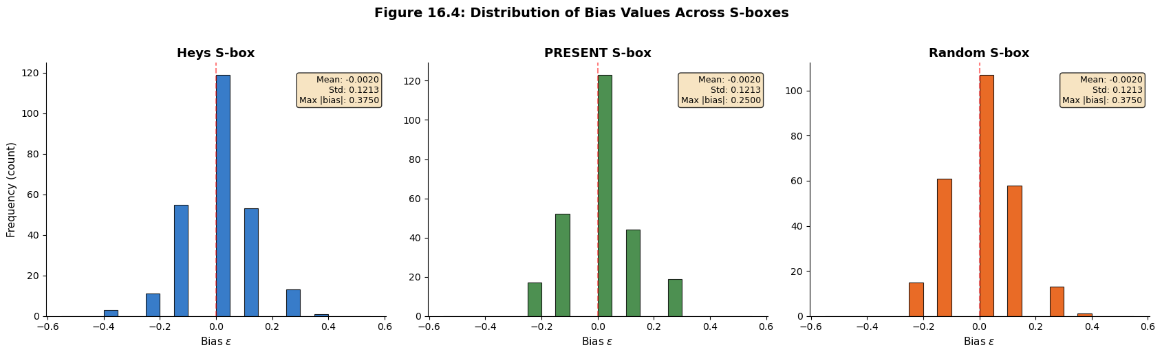
16.8 Distribution of Bias Values#
For a “good” S-box (one that resists linear cryptanalysis), the bias values should be concentrated near zero, with only a few entries having large absolute bias. Let us examine the distribution of bias values across all three S-boxes and compare them to the theoretical distribution for a random function.
Show code cell source
import numpy as np
import matplotlib.pyplot as plt

def compute_lat(sbox):
    sbox = np.array(sbox, dtype=int)
    n = len(sbox)
    n_out = 2**int(np.log2(max(sbox) + 1))
    half = n // 2
    lat = np.zeros((n, n_out), dtype=int)
    for alpha in range(n):
        for beta in range(n_out):
            count = 0
            for x in range(n):
                lhs = bin(alpha & x).count('1') % 2
                rhs = bin(beta & sbox[x]).count('1') % 2
                if lhs == rhs:
                    count += 1
            lat[alpha][beta] = count - half
    return lat

HEYS_SBOX = [0xE, 0x4, 0xD, 0x1, 0x2, 0xF, 0xB, 0x8,
             0x3, 0xA, 0x6, 0xC, 0x5, 0x9, 0x0, 0x7]
PRESENT_SBOX = [0xC, 0x5, 0x6, 0xB, 0x9, 0x0, 0xA, 0xD,
                0x3, 0xE, 0xF, 0x8, 0x4, 0x7, 0x1, 0x2]
np.random.seed(2023)
RANDOM_SBOX = list(np.random.permutation(16))

sboxes = {'Heys': HEYS_SBOX, 'PRESENT': PRESENT_SBOX, 'Random': RANDOM_SBOX}
colors = {'Heys': '#1565C0', 'PRESENT': '#2E7D32', 'Random': '#E65100'}

fig, axes = plt.subplots(1, 3, figsize=(17, 5))

for idx, (name, sbox) in enumerate(sboxes.items()):
    lat = compute_lat(sbox)
    n = len(sbox)

    # Collect all bias values (excluding trivial (0,0) entry)
    biases = []
    for a in range(n):
        for b in range(n):
            if a == 0 and b == 0:
                continue
            biases.append(lat[a][b] / n)

    biases = np.array(biases)

    # Histogram
    bins = np.linspace(-0.55, 0.55, 23)
    axes[idx].hist(biases, bins=bins, color=colors[name], edgecolor='black',
                   linewidth=0.8, alpha=0.85, density=False)
    axes[idx].set_title(f'{name} S-box', fontsize=13, fontweight='bold')
    axes[idx].set_xlabel('Bias $\\varepsilon$', fontsize=11)
    if idx == 0:
        axes[idx].set_ylabel('Frequency (count)', fontsize=11)
    axes[idx].axvline(x=0, color='red', linestyle='--', alpha=0.5, linewidth=1.5)

    # Statistics
    axes[idx].text(0.98, 0.95,
                   f'Mean: {np.mean(biases):+.4f}\n'
                   f'Std: {float(np.std(biases)):.4f}\n'
                   f'Max |bias|: {float(np.max(np.abs(biases))):.4f}',
                   transform=axes[idx].transAxes, fontsize=9,
                   verticalalignment='top', horizontalalignment='right',
                   bbox=dict(boxstyle='round', facecolor='wheat', alpha=0.8))

    axes[idx].spines['top'].set_visible(False)
    axes[idx].spines['right'].set_visible(False)

fig.suptitle('Figure 16.4: Distribution of Bias Values Across S-boxes',
             fontsize=14, fontweight='bold', y=1.02)

plt.tight_layout()
plt.savefig('fig_16_4_bias_distribution.png', dpi=150, bbox_inches='tight', facecolor='white')
plt.show()
16.9 Nonlinearity and the Walsh-Hadamard Transform#
The LAT is intimately related to the Walsh-Hadamard transform, which provides an efficient way to compute all entries simultaneously. The nonlinearity of an S-box – a key design metric – is defined in terms of the maximum absolute value in the LAT.
Definition 16.4 (Nonlinearity of an S-box)
The nonlinearity of an S-box \(S: \mathbb{F}_2^n \to \mathbb{F}_2^n\) is:
Higher nonlinearity means better resistance to linear cryptanalysis. For a 4-bit S-box (\(n = 4\)), the maximum achievable nonlinearity is \(2^{n-1} - 2^{n/2-1} = 8 - 2 = 4\) (in the LAT-count metric, this means \(\max |\Lambda| = 4\)).
Let us compute the nonlinearity of our three S-boxes and verify with the Walsh-Hadamard approach.
Show code cell source
import numpy as np
import matplotlib.pyplot as plt

def compute_lat(sbox):
    sbox = np.array(sbox, dtype=int)
    n = len(sbox)
    n_out = 2**int(np.log2(max(sbox) + 1))
    half = n // 2
    lat = np.zeros((n, n_out), dtype=int)
    for alpha in range(n):
        for beta in range(n_out):
            count = 0
            for x in range(n):
                lhs = bin(alpha & x).count('1') % 2
                rhs = bin(beta & sbox[x]).count('1') % 2
                if lhs == rhs:
                    count += 1
            lat[alpha][beta] = count - half
    return lat

def walsh_hadamard_lat(sbox):
    """
    Compute the LAT using the Walsh-Hadamard transform.

    For each output mask beta, define the Boolean function
    f_beta(x) = <beta, S(x)>. The Walsh-Hadamard coefficient is:
        W_f(alpha) = sum_x (-1)^{<alpha,x> XOR f_beta(x)}

    Then LAT[alpha][beta] = W_f(alpha) / 2
    """
    sbox = np.array(sbox, dtype=int)
    n = len(sbox)
    n_bits = int(np.log2(n))
    n_out = 2**int(np.log2(max(sbox) + 1))
    lat = np.zeros((n, n_out), dtype=int)

    for beta in range(n_out):
        # Build truth table of f_beta(x) = <beta, S(x)>
        f = np.array([bin(beta & sbox[x]).count('1') % 2 for x in range(n)])

        for alpha in range(n):
            # Compute Walsh coefficient
            walsh = 0
            for x in range(n):
                ax = bin(alpha & x).count('1') % 2
                walsh += (-1)**(ax ^ f[x])
            lat[alpha][beta] = walsh // 2

    return lat

HEYS_SBOX = [0xE, 0x4, 0xD, 0x1, 0x2, 0xF, 0xB, 0x8,
             0x3, 0xA, 0x6, 0xC, 0x5, 0x9, 0x0, 0x7]
PRESENT_SBOX = [0xC, 0x5, 0x6, 0xB, 0x9, 0x0, 0xA, 0xD,
                0x3, 0xE, 0xF, 0x8, 0x4, 0x7, 0x1, 0x2]
np.random.seed(2023)
RANDOM_SBOX = list(np.random.permutation(16))

sboxes = {'Heys': HEYS_SBOX, 'PRESENT': PRESENT_SBOX, 'Random': RANDOM_SBOX}

print("Nonlinearity Analysis")
print("=" * 60)
print()

for name, sbox in sboxes.items():
    lat_direct = compute_lat(sbox)
    lat_walsh = walsh_hadamard_lat(sbox)

    # Verify both methods agree
    assert np.array_equal(lat_direct, lat_walsh), f"Mismatch for {name}!"

    n = len(sbox)
    # Max absolute LAT entry (excluding (0,0))
    max_lat = 0
    for a in range(n):
        for b in range(n):
            if a == 0 and b == 0:
                continue
            max_lat = max(max_lat, abs(lat_direct[a][b]))

    nonlinearity = (n // 2) - max_lat
    max_bias = max_lat / n

    print(f"  {name:10s} S-box:")
    print(f"    Max |LAT entry|      = {max_lat}")
    print(f"    Nonlinearity NL(S)   = {n//2} - {max_lat} = {nonlinearity}")
    print(f"    Max |bias|           = {float(max_bias):.4f}")
    print(f"    Walsh methods agree  = True")
    print()

print("Verification: direct LAT computation and Walsh-Hadamard give identical results.")
print()

# Visualize nonlinearity comparison as a bar chart
names = list(sboxes.keys())
nonlinearities = []
max_biases = []
for name, sbox in sboxes.items():
    lat = compute_lat(sbox)
    n = len(sbox)
    max_lat = max(abs(lat[a][b]) for a in range(n) for b in range(n)
                  if not (a == 0 and b == 0))
    nonlinearities.append((n // 2) - max_lat)
    max_biases.append(max_lat / n)

fig, axes = plt.subplots(1, 2, figsize=(12, 5))

colors = ['#1565C0', '#2E7D32', '#E65100']

# Nonlinearity
bars1 = axes[0].bar(names, nonlinearities, color=colors, edgecolor='black', linewidth=1)
axes[0].set_ylabel('Nonlinearity $\\mathcal{NL}(S)$', fontsize=12)
axes[0].set_title('S-box Nonlinearity', fontsize=13, fontweight='bold')
axes[0].axhline(y=4, color='red', linestyle='--', alpha=0.6, label='Optimal (NL=4)')
axes[0].legend(fontsize=10)
for bar, nl in zip(bars1, nonlinearities):
    axes[0].text(bar.get_x() + bar.get_width()/2, bar.get_height() + 0.1,
                 str(nl), ha='center', fontweight='bold', fontsize=12)
axes[0].set_ylim(0, 5.5)
axes[0].spines['top'].set_visible(False)
axes[0].spines['right'].set_visible(False)

# Max absolute bias
bars2 = axes[1].bar(names, max_biases, color=colors, edgecolor='black', linewidth=1)
axes[1].set_ylabel('Max $|\\varepsilon|$', fontsize=12)
axes[1].set_title('Maximum Absolute Bias', fontsize=13, fontweight='bold')
axes[1].axhline(y=0.25, color='red', linestyle='--', alpha=0.6, label='Optimal bound (1/4)')
axes[1].legend(fontsize=10)
for bar, mb in zip(bars2, max_biases):
    axes[1].text(bar.get_x() + bar.get_width()/2, bar.get_height() + 0.005,
                 f'{float(mb):.3f}', ha='center', fontweight='bold', fontsize=11)
axes[1].set_ylim(0, 0.55)
axes[1].spines['top'].set_visible(False)
axes[1].spines['right'].set_visible(False)

fig.suptitle('Figure 16.5: S-box Quality Metrics for Linear Cryptanalysis Resistance',
             fontsize=14, fontweight='bold', y=1.02)

plt.tight_layout()
plt.savefig('fig_16_5_nonlinearity_comparison.png', dpi=150, bbox_inches='tight', facecolor='white')
plt.show()
Nonlinearity Analysis
============================================================

  Heys       S-box:
    Max |LAT entry|      = 6
    Nonlinearity NL(S)   = 8 - 6 = 2
    Max |bias|           = 0.3750
    Walsh methods agree  = True

  PRESENT    S-box:
    Max |LAT entry|      = 4
    Nonlinearity NL(S)   = 8 - 4 = 4
    Max |bias|           = 0.2500
    Walsh methods agree  = True

  Random     S-box:
    Max |LAT entry|      = 6
    Nonlinearity NL(S)   = 8 - 6 = 2
    Max |bias|           = 0.3750
    Walsh methods agree  = True

Verification: direct LAT computation and Walsh-Hadamard give identical results.
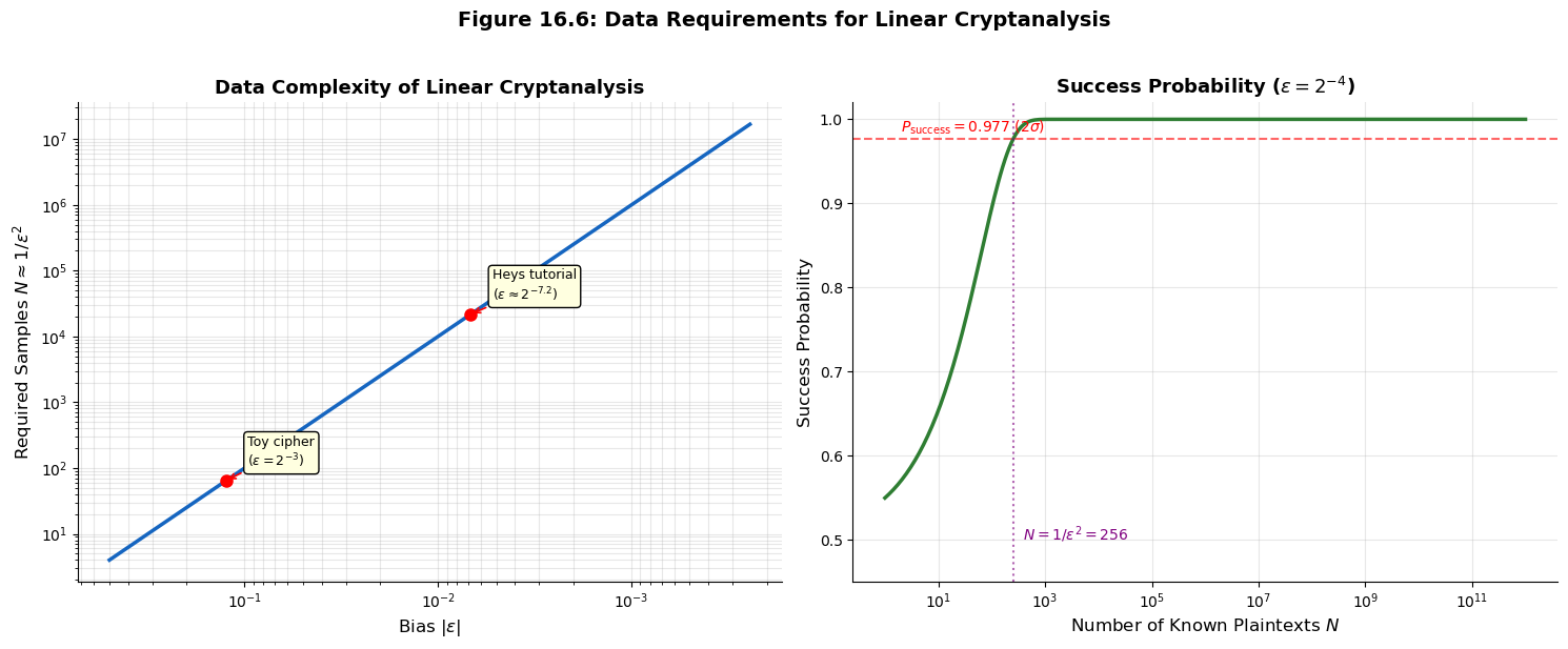
16.10 Data Complexity of Linear Cryptanalysis#
A crucial question for the practitioner is: how many known plaintexts are needed to exploit a linear approximation with bias \(\varepsilon\)? The answer comes from a statistical argument based on the Central Limit Theorem.
Theorem 16.2 (Data Complexity)
To distinguish a linear approximation with bias \(\varepsilon\) from a random guess (bias 0) with success probability \(\geq 97.7\%\), the number of known plaintext-ciphertext pairs required is approximately:
More precisely, using a sign-determination test, the success probability after \(N\) samples is:
where \(\Phi\) is the standard normal CDF. Setting \(P_{\text{success}} = 0.977\) (corresponding to \(2\sigma\)) gives \(N \approx 1/\varepsilon^2\).
This inverse-square relationship means that halving the bias requires four times as many plaintexts. For Matsui’s attack on DES, the best linear approximation across 14 rounds had bias \(|\varepsilon| \approx 2^{-21.2}\), yielding a data requirement of approximately \(2^{42.4} \approx 2^{43}\) known plaintexts.
Show code cell source
import numpy as np
import matplotlib.pyplot as plt

# We implement the normal CDF using the error function from numpy
# Phi(x) = 0.5 * (1 + erf(x / sqrt(2)))
from numpy import sqrt, log2

def normal_cdf(x):
    """Standard normal CDF using the error function."""
    return 0.5 * (1.0 + np.vectorize(lambda v: np.math.erf(v / np.sqrt(2)))(x))

# Data complexity as a function of bias
biases = np.logspace(-1, -12, 200, base=2)  # from 2^{-1} to 2^{-12}
data_required = 1.0 / biases**2

fig, axes = plt.subplots(1, 2, figsize=(15, 6))

# Left: Data complexity vs bias (log-log)
axes[0].loglog(biases, data_required, color='#1565C0', linewidth=2.5)
axes[0].set_xlabel('Bias $|\\varepsilon|$', fontsize=12)
axes[0].set_ylabel('Required Samples $N \\approx 1/\\varepsilon^2$', fontsize=12)
axes[0].set_title('Data Complexity of Linear Cryptanalysis', fontsize=13, fontweight='bold')
axes[0].grid(True, alpha=0.3, which='both')
axes[0].invert_xaxis()

# Mark specific points
notable = [
    (2**-3, 'Toy cipher\n($\\varepsilon = 2^{-3}$)'),
    (2**-7.2, 'Heys tutorial\n($\\varepsilon \\approx 2^{-7.2}$)'),
]
for eps_val, label in notable:
    n_val = 1.0 / eps_val**2
    axes[0].plot(eps_val, n_val, 'ro', markersize=8, zorder=5)
    axes[0].annotate(label, (eps_val, n_val),
                     textcoords="offset points", xytext=(15, 10),
                     fontsize=9, ha='left',
                     arrowprops=dict(arrowstyle='->', color='red', lw=1.2),
                     bbox=dict(boxstyle='round,pad=0.3', facecolor='lightyellow'))

axes[0].spines['top'].set_visible(False)
axes[0].spines['right'].set_visible(False)

# Right: Success probability vs N for a fixed bias
eps_fixed = 2**-4  # bias = 1/16
N_values = np.logspace(0, 12, 300)
success_probs = normal_cdf(2 * eps_fixed * np.sqrt(N_values))

axes[1].semilogx(N_values, success_probs, color='#2E7D32', linewidth=2.5)
axes[1].set_xlabel('Number of Known Plaintexts $N$', fontsize=12)
axes[1].set_ylabel('Success Probability', fontsize=12)
axes[1].set_title(f'Success Probability ($\\varepsilon = 2^{{-4}}$)', fontsize=13, fontweight='bold')
axes[1].axhline(y=0.977, color='red', linestyle='--', alpha=0.6, linewidth=1.5)
axes[1].text(2, 0.985, '$P_{\\mathrm{success}} = 0.977$ ($2\\sigma$)', fontsize=10, color='red')

# Mark N = 1/eps^2
N_threshold = 1.0 / eps_fixed**2
axes[1].axvline(x=N_threshold, color='purple', linestyle=':', alpha=0.6, linewidth=1.5)
axes[1].text(N_threshold * 1.5, 0.5, f'$N = 1/\\varepsilon^2 = {int(N_threshold)}$',
             fontsize=10, color='purple', rotation=0)

axes[1].set_ylim(0.45, 1.02)
axes[1].grid(True, alpha=0.3)
axes[1].spines['top'].set_visible(False)
axes[1].spines['right'].set_visible(False)

fig.suptitle('Figure 16.6: Data Requirements for Linear Cryptanalysis',
             fontsize=14, fontweight='bold', y=1.02)

plt.tight_layout()
plt.savefig('fig_16_6_data_complexity.png', dpi=150, bbox_inches='tight', facecolor='white')
plt.show()
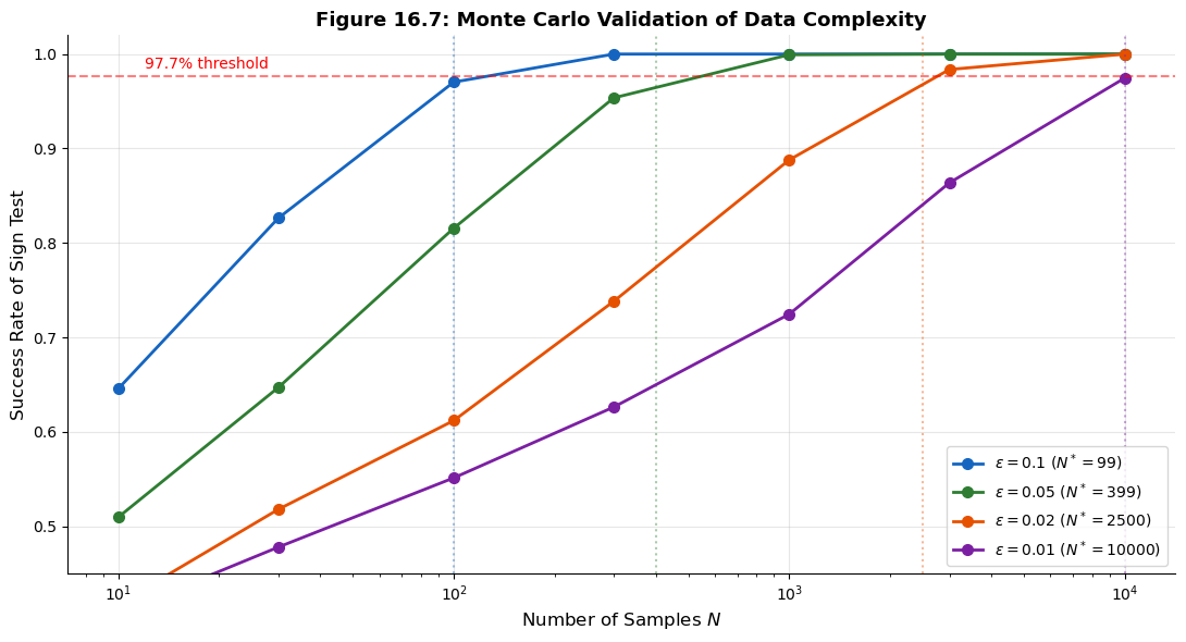
Monte Carlo Validation of the Data Complexity Bound#
Let us verify the \(N \approx 1/\varepsilon^2\) bound experimentally. We simulate a linear approximation with known bias and measure the success rate of the sign-determination test as a function of the sample size.
Show code cell source
import numpy as np
import matplotlib.pyplot as plt

np.random.seed(42)

def run_sign_test(true_bias, n_samples, n_trials=5000):
    """
    Simulate the sign-determination test.

    For each trial:
    1. Generate n_samples biased bits (P(X=0) = 0.5 + true_bias)
    2. Estimate the bias from the sample
    3. Check if the sign of the estimate matches the true sign

    Returns the fraction of trials where the sign is correct.
    """
    correct = 0
    for _ in range(n_trials):
        bits = (np.random.random(n_samples) >= (0.5 + true_bias)).astype(int)
        estimated_bias = np.mean(bits == 0) - 0.5
        if np.sign(estimated_bias) == np.sign(true_bias):
            correct += 1
    return correct / n_trials

# Test with several bias values
test_biases = [0.1, 0.05, 0.02, 0.01]
sample_sizes = [10, 30, 100, 300, 1000, 3000, 10000]

fig, ax = plt.subplots(figsize=(11, 6))

colors = ['#1565C0', '#2E7D32', '#E65100', '#7B1FA2']

for i, eps in enumerate(test_biases):
    success_rates = []
    for n_s in sample_sizes:
        sr = run_sign_test(eps, n_s, n_trials=3000)
        success_rates.append(sr)

    # Theoretical prediction
    N_theory = 1.0 / eps**2

    ax.semilogx(sample_sizes, success_rates, 'o-', color=colors[i], linewidth=2,
                markersize=7, label=f'$\\varepsilon = {eps}$ ($N^* = {int(N_theory)}$)')

    # Mark theoretical threshold
    ax.axvline(x=N_theory, color=colors[i], linestyle=':', alpha=0.4, linewidth=1.5)

ax.axhline(y=0.977, color='red', linestyle='--', alpha=0.5, linewidth=1.5)
ax.text(12, 0.985, '97.7% threshold', fontsize=10, color='red')

ax.set_xlabel('Number of Samples $N$', fontsize=12)
ax.set_ylabel('Success Rate of Sign Test', fontsize=12)
ax.set_title('Figure 16.7: Monte Carlo Validation of Data Complexity',
             fontsize=13, fontweight='bold')
ax.legend(fontsize=10, loc='lower right')
ax.set_ylim(0.45, 1.02)
ax.grid(True, alpha=0.3)
ax.spines['top'].set_visible(False)
ax.spines['right'].set_visible(False)

plt.tight_layout()
plt.savefig('fig_16_7_monte_carlo_validation.png', dpi=150, bbox_inches='tight', facecolor='white')
plt.show()
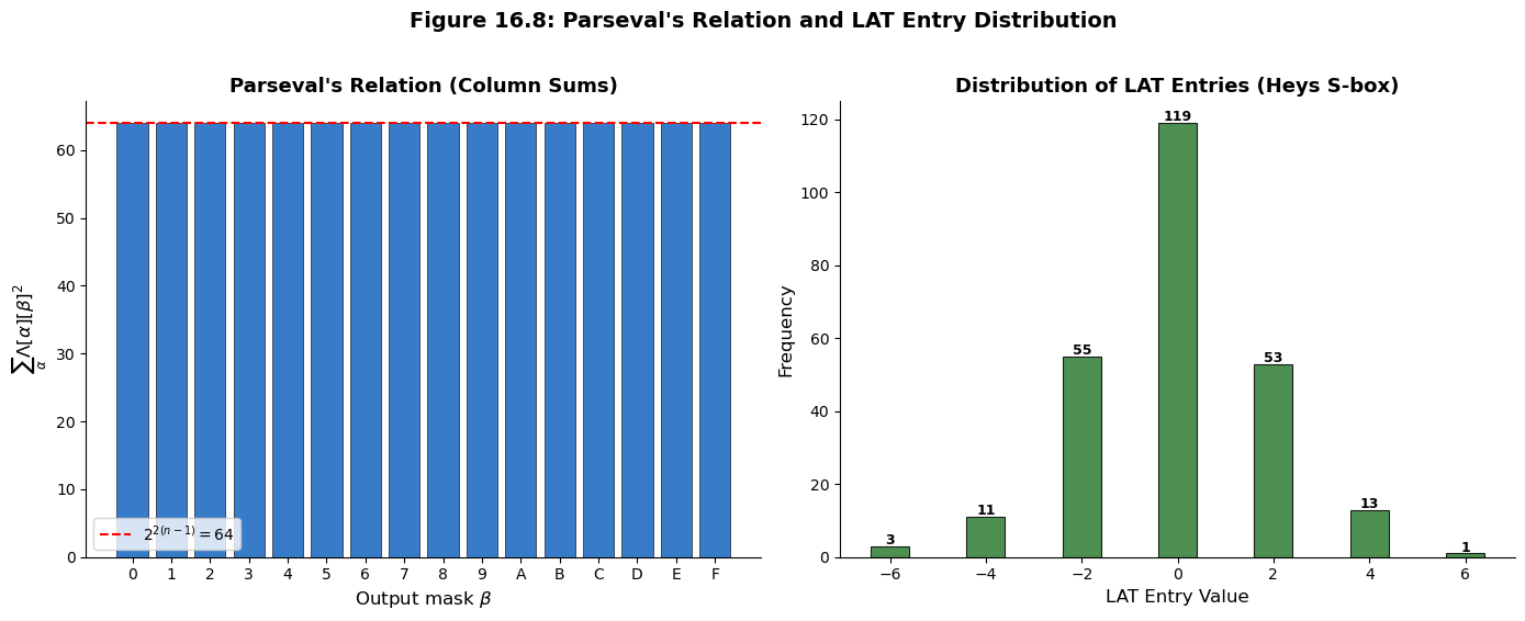
16.11 Statistical Properties of the LAT#
The entries of the LAT are not arbitrary integers – they obey specific structural constraints. Understanding these constraints is important both for S-box design and for assessing the quality of linear approximations.
Theorem 16.3 (Parseval’s Relation for the LAT)
For any S-box \(S: \mathbb{F}_2^n \to \mathbb{F}_2^n\) (a permutation), and for any fixed output mask \(\beta \neq 0\):
This is the Parseval relation, and it implies that the “energy” in each column of the LAT is fixed. If one entry is large, others must be correspondingly smaller.
Let us verify Parseval’s relation numerically for our S-boxes.
Show code cell source
import numpy as np
import matplotlib.pyplot as plt

def compute_lat(sbox):
    sbox = np.array(sbox, dtype=int)
    n = len(sbox)
    n_out = 2**int(np.log2(max(sbox) + 1))
    half = n // 2
    lat = np.zeros((n, n_out), dtype=int)
    for alpha in range(n):
        for beta in range(n_out):
            count = 0
            for x in range(n):
                lhs = bin(alpha & x).count('1') % 2
                rhs = bin(beta & sbox[x]).count('1') % 2
                if lhs == rhs:
                    count += 1
            lat[alpha][beta] = count - half
    return lat

HEYS_SBOX = [0xE, 0x4, 0xD, 0x1, 0x2, 0xF, 0xB, 0x8,
             0x3, 0xA, 0x6, 0xC, 0x5, 0x9, 0x0, 0x7]

lat = compute_lat(HEYS_SBOX)
n = 16  # 2^4

print("Parseval's Relation Verification for the Heys S-box")
print("=" * 55)
print()
print(f"Expected: sum_alpha LAT[alpha][beta]^2 = 2^{{2(n-1)}} = 2^6 = {2**6}")
print()

# Check for each non-zero beta
print(f"{'beta':>6s}  {'Sum of squares':>16s}  {'Expected':>10s}  {'Match':>6s}")
print("-" * 46)

all_match = True
for beta in range(1, 16):
    col_sum_sq = sum(int(lat[alpha][beta])**2 for alpha in range(16))
    expected = 2**6  # = 64
    match = col_sum_sq == expected
    if not match:
        all_match = False
    print(f"0x{beta:01X}     {int(col_sum_sq):16d}  {int(expected):10d}  {'Yes' if match else 'NO':>6s}")

print()
print(f"All columns satisfy Parseval's relation: {all_match}")
print()

# Similarly check row sums for non-zero alpha
print("Row-wise check (fixed alpha, sum over beta):")
print(f"{'alpha':>6s}  {'Sum of squares':>16s}")
print("-" * 28)
for alpha in range(1, 16):
    row_sum_sq = sum(int(lat[alpha][beta])**2 for beta in range(16))
    print(f"0x{alpha:01X}     {int(row_sum_sq):16d}")

print()
print("Note: Row sums also equal 64 = 2^6 for this permutation S-box.")
print("This is because Parseval's relation holds both row-wise and column-wise")
print("for bijective S-boxes.")

# Visualization: energy distribution across columns
fig, axes = plt.subplots(1, 2, figsize=(14, 5.5))

# Column energy breakdown
beta_values = list(range(16))
col_energies = []
for beta in beta_values:
    col_sq = sum(int(lat[alpha][beta])**2 for alpha in range(16))
    col_energies.append(col_sq)
    axes[0].bar(beta, col_sq, color='#1565C0',
                edgecolor='black', linewidth=0.5, alpha=0.85)

axes[0].axhline(y=64, color='red', linestyle='--', linewidth=1.5, label='$2^{2(n-1)} = 64$')
axes[0].set_xlabel('Output mask $\\beta$', fontsize=12)
axes[0].set_ylabel('$\\sum_{\\alpha} \\Lambda[\\alpha][\\beta]^2$', fontsize=12)
axes[0].set_title("Parseval's Relation (Column Sums)", fontsize=13, fontweight='bold')
axes[0].set_xticks(range(16))
axes[0].set_xticklabels([f'{i:X}' for i in range(16)])
axes[0].legend(fontsize=10)
axes[0].spines['top'].set_visible(False)
axes[0].spines['right'].set_visible(False)

# Distribution of LAT entries (all non-trivial)
all_entries = []
for a in range(16):
    for b in range(16):
        if a == 0 and b == 0:
            continue
        all_entries.append(int(lat[a][b]))

unique_vals = sorted(set(all_entries))
counts = [all_entries.count(v) for v in unique_vals]

axes[1].bar(unique_vals, counts, color='#2E7D32', edgecolor='black', linewidth=0.8, alpha=0.85)
axes[1].set_xlabel('LAT Entry Value', fontsize=12)
axes[1].set_ylabel('Frequency', fontsize=12)
axes[1].set_title('Distribution of LAT Entries (Heys S-box)', fontsize=13, fontweight='bold')
axes[1].spines['top'].set_visible(False)
axes[1].spines['right'].set_visible(False)

# Annotate
for v, c in zip(unique_vals, counts):
    if c > 0:
        axes[1].text(v, c + 0.5, str(c), ha='center', fontsize=9, fontweight='bold')

fig.suptitle("Figure 16.8: Parseval's Relation and LAT Entry Distribution",
             fontsize=14, fontweight='bold', y=1.02)

plt.tight_layout()
plt.savefig('fig_16_8_parseval_verification.png', dpi=150, bbox_inches='tight', facecolor='white')
plt.show()
Parseval's Relation Verification for the Heys S-box
=======================================================

Expected: sum_alpha LAT[alpha][beta]^2 = 2^{2(n-1)} = 2^6 = 64

  beta    Sum of squares    Expected   Match
----------------------------------------------
0x1                   64          64     Yes
0x2                   64          64     Yes
0x3                   64          64     Yes
0x4                   64          64     Yes
0x5                   64          64     Yes
0x6                   64          64     Yes
0x7                   64          64     Yes
0x8                   64          64     Yes
0x9                   64          64     Yes
0xA                   64          64     Yes
0xB                   64          64     Yes
0xC                   64          64     Yes
0xD                   64          64     Yes
0xE                   64          64     Yes
0xF                   64          64     Yes

All columns satisfy Parseval's relation: True

Row-wise check (fixed alpha, sum over beta):
 alpha    Sum of squares
----------------------------
0x1                   64
0x2                   64
0x3                   64
0x4                   64
0x5                   64
0x6                   64
0x7                   64
0x8                   64
0x9                   64
0xA                   64
0xB                   64
0xC                   64
0xD                   64
0xE                   64
0xF                   64

Note: Row sums also equal 64 = 2^6 for this permutation S-box.
This is because Parseval's relation holds both row-wise and column-wise
for bijective S-boxes.
16.12 Exercises#
Exercise 16.1 (Computing the LAT by Hand). Consider the 3-bit S-box \(S: \mathbb{F}_2^3 \to \mathbb{F}_2^3\) defined by:
\(x\) |
0 |
1 |
2 |
3 |
4 |
5 |
6 |
7 |
|---|---|---|---|---|---|---|---|---|
\(S(x)\) |
6 |
4 |
0 |
3 |
7 |
2 |
1 |
5 |
(a) Compute the full \(8 \times 8\) LAT of this S-box by hand (or by systematic calculation). Show your work for at least three non-trivial entries.
(b) Identify the linear approximation with the largest absolute bias. What are \(\alpha\), \(\beta\), and \(\varepsilon\)?
(c) If this S-box were used in a 4-round SPN cipher with no other sources of diffusion, what would the piling-up lemma predict for the bias of a 4-round linear approximation built from copies of your best single-round approximation?
Hint
For each entry \(\Lambda[\alpha][\beta]\), iterate over all 8 inputs \(x \in \{0, \ldots, 7\}\) and count how many satisfy \(\langle \alpha, x \rangle = \langle \beta, S(x) \rangle\). Then subtract \(2^{n-1} = 4\).
For part (c), if the best single-round bias is \(\varepsilon_1\), then by the piling-up lemma the 4-round bias is \(\varepsilon_4 = 2^3 \cdot \varepsilon_1^4\).
Exercise 16.2 (Piling-Up Lemma: Edge Cases).
(a) Prove that if any one of the \(n\) independent binary random variables \(X_i\) is perfectly balanced (i.e., \(\varepsilon_i = 0\)), then the bias of \(X_1 \oplus \cdots \oplus X_n\) is exactly zero, regardless of the other biases. Interpret this result in the context of cipher design.
(b) Prove that if all \(n\) variables have the same bias \(\varepsilon\), then the combined bias is \(\varepsilon_{\text{total}} = 2^{n-1} \varepsilon^n\). For what value of \(n\) does \(|\varepsilon_{\text{total}}|\) begin to decrease as a function of \(n\) (assuming \(|\varepsilon| < 1/2\))?
(c) Matsui’s attack on DES uses a 14-round linear approximation. If the average per-round bias is \(|\varepsilon_r| \approx 2^{-2}\), estimate the total bias and the required number of known plaintexts. Compare this to the reported \(2^{43}\).
Hint
For (a), if \(\varepsilon_i = 0\) for any \(i\), the product \(\prod \varepsilon_j\) contains a zero factor.
For (b), differentiate \(f(n) = 2^{n-1} \varepsilon^n\) with respect to \(n\) (treating \(n\) as continuous) and set \(f'(n) = 0\). Alternatively, note that \(f(n) = \frac{1}{2}(2\varepsilon)^n\), so \(|f(n)|\) decreases when \(|2\varepsilon| < 1\), i.e., \(|\varepsilon| < 1/2\) – which means it decreases for all \(n \geq 1\).
For (c), be careful: the 14-round approximation is not simply 14 copies of the same one-round approximation. The actual construction uses a chain of different S-box approximations.
Exercise 16.3 (S-box Design Criteria).
Design a 4-bit S-box \(S: \mathbb{F}_2^4 \to \mathbb{F}_2^4\) (a permutation of \(\{0, \ldots, 15\}\)) that achieves optimal nonlinearity for linear cryptanalysis resistance (i.e., \(\mathcal{NL}(S) = 4\), meaning the maximum absolute LAT entry is 4).
(a) Verify your S-box by computing its full LAT and confirming that no entry (excluding \(\Lambda[0][0]\)) exceeds 4 in absolute value.
(b) Is your S-box also optimal with respect to differential cryptanalysis resistance? (You may use tools from a later chapter, or simply check whether the maximum entry in the Difference Distribution Table exceeds 4.)
(c) Explain why it is impossible to have all non-trivial LAT entries equal to \(\pm 2\) for a 4-bit S-box. (Hint: use Parseval’s relation.)
Hint
The PRESENT S-box [0xC, 0x5, 0x6, 0xB, 0x9, 0x0, 0xA, 0xD, 0x3, 0xE, 0xF, 0x8, 0x4, 0x7, 0x1, 0x2] is known to achieve optimal nonlinearity.
For (c), Parseval says \(\sum_\alpha \Lambda[\alpha][\beta]^2 = 64\) for each non-zero \(\beta\). If all 16 entries (including \(\alpha = 0\)) were \(\pm 2\), the sum would be \(16 \times 4 = 64\). But \(\Lambda[0][\beta] = 0\) for any non-zero \(\beta\) when \(S\) is a permutation, so you only have 15 non-zero-alpha entries, giving \(15 \times 4 = 60 \neq 64\). This is a contradiction.
Exercise 16.4 (Linear Approximations of Composed Functions).
Let \(S_1: \mathbb{F}_2^4 \to \mathbb{F}_2^4\) and \(S_2: \mathbb{F}_2^4 \to \mathbb{F}_2^4\) be two S-boxes, and define \(T = S_2 \circ S_1\).
(a) Write a Python function that computes the LAT of \(T\) directly from the LATs of \(S_1\) and \(S_2\) using the composition formula:
(b) Verify your formula by comparing the result to the LAT computed directly from the composed S-box lookup table.
(c) Explain the connection between this composition formula and the piling-up lemma. Under what conditions does the formula give exact results vs. approximate results?
Hint
The composition formula is a matrix multiplication (up to a scaling factor). It is exact when the intermediate values are uniformly distributed (i.e., when \(S_1\) is a permutation). The piling-up lemma is the special case where you approximate the product of two biases as \(2 \varepsilon_1 \varepsilon_2\).
In matrix form: \(\Lambda_T = \frac{1}{2^{n-1}} \Lambda_{S_1} \cdot \Lambda_{S_2}\).
Exercise 16.5 (Challenge: From LAT to Key Recovery).
Consider a simplified 2-round SPN cipher with:
Block size: 4 bits
S-box: the Heys S-box
[0xE, 0x4, 0xD, 0x1, 0x2, 0xF, 0xB, 0x8, 0x3, 0xA, 0x6, 0xC, 0x5, 0x9, 0x0, 0x7]No permutation layer (identity permutation)
Three round keys \(K_0, K_1, K_2 \in \mathbb{F}_2^4\) XORed before/between/after the S-box layers
The encryption is: \(C = S(S(P \oplus K_0) \oplus K_1) \oplus K_2\)
(a) Using the LAT, find the best linear approximation across the 2-round cipher (one approximation per S-box application, combined via the piling-up lemma).
(b) Write a Python program that:
Encrypts 1000 random plaintexts under a random key \((K_0, K_1, K_2)\)
For each candidate value of \(K_2\), partially decrypts the ciphertext through the last round
Counts the bias of the linear approximation for each candidate \(K_2\)
Recovers \(K_2\) as the candidate with the largest absolute bias
(c) How many known plaintexts are needed to recover \(K_2\) with \(> 95\%\) success rate? Verify experimentally.
Hint
The best approximation for the Heys S-box has bias \(\pm 1/4\). Using the piling-up lemma for 2 rounds: \(\varepsilon_{2r} = 2 \cdot (1/4) \cdot (1/4) = 1/8\). So \(N \approx 1/(1/8)^2 = 64\) plaintexts should suffice.
For the key recovery: partially decrypt with each of the 16 candidate values of \(K_2\), apply the inverse S-box, and check which candidate gives the strongest bias for the linear approximation. The correct \(K_2\) will produce a distinctly larger bias than incorrect candidates.
16.13 Summary#
This chapter has laid the mathematical and computational foundations of linear cryptanalysis, one of the two most important general-purpose attacks on block ciphers (the other being differential cryptanalysis, which we study in Chapter 17).
Key concepts introduced:
Linear approximation – a probabilistic linear equation relating input bits, output bits, and key bits of a cipher component. Characterized by input mask \(\alpha\), output mask \(\beta\), and bias \(\varepsilon\).
Bias – the deviation \(\varepsilon = \Pr[\langle \alpha, x \rangle = \langle \beta, S(x) \rangle] - 1/2\) that measures how far a linear approximation deviates from random. Large \(|\varepsilon|\) means the S-box is “more linear” along that approximation.
Linear Approximation Table (LAT) – the complete catalog of all biases for all mask pairs. The LAT is to linear cryptanalysis what the DDT (Difference Distribution Table) is to differential cryptanalysis.
Piling-up lemma – the composition rule \(\varepsilon_{1 \oplus \cdots \oplus n} = 2^{n-1}\prod \varepsilon_i\) that allows biases of individual round approximations to be combined into a multi-round approximation.
Nonlinearity – the key S-box design metric \(\mathcal{NL}(S) = 2^{n-1} - \max|\Lambda[\alpha][\beta]|\) that quantifies resistance to linear cryptanalysis.
Data complexity – the number of known plaintexts \(N \approx 1/\varepsilon^2\) required to exploit a linear approximation.
Parseval’s relation – the constraint \(\sum_\alpha \Lambda[\alpha][\beta]^2 = 2^{2(n-1)}\) that limits how “nonlinear” an S-box can be.
Tip
Looking ahead. In Chapter 17, we will apply these foundations to mount a complete linear attack on a simplified SPN cipher, following Heys’ tutorial. We will construct multi-round linear approximations, implement the key-recovery phase, and analyze the success probability as a function of the number of known plaintexts.
16.14 References#
Mitsuru Matsui, “Linear Cryptanalysis Method for DES Cipher,” Advances in Cryptology – EUROCRYPT ‘93, Lecture Notes in Computer Science, vol. 765, pp. 386–397, Springer, 1994. The foundational paper introducing linear cryptanalysis. Matsui presents the piling-up lemma, constructs linear approximations for DES, and outlines Algorithm 1 (basic key recovery) and Algorithm 2 (improved key recovery).
Mitsuru Matsui, “The First Experimental Cryptanalysis of the Data Encryption Standard,” Advances in Cryptology – CRYPTO ‘94, Lecture Notes in Computer Science, vol. 839, pp. 1–11, Springer, 1994. Matsui’s follow-up paper reporting the first successful experimental linear cryptanalysis of full DES, recovering the 56-bit key using \(2^{43}\) known plaintexts on a set of 12 HP 9735 workstations.
Howard M. Heys, “A Tutorial on Linear and Differential Cryptanalysis,” Cryptologia, 26(3), pp. 189–221, 2002. An excellent pedagogical introduction to both linear and differential cryptanalysis, using a simplified SPN cipher as the running example. The Heys S-box used throughout this chapter comes from this tutorial. Highly recommended as a companion to this chapter.
Eli Biham and Adi Shamir, “Differential Cryptanalysis of DES-like Cryptosystems,” Journal of Cryptology, 4(1), pp. 3–72, 1991. While focused on differential cryptanalysis, this paper provides essential context for understanding why linear cryptanalysis was such an important development – it was the second general attack methodology for Feistel ciphers.
Joan Daemen and Vincent Rijmen, The Design of Rijndael: AES – The Advanced Encryption Standard, Springer, 2002. The designers of AES explain the wide trail strategy, which was explicitly designed to provide provable bounds against both linear and differential cryptanalysis. Chapter 9 discusses the relationship between S-box properties (including the LAT) and cipher security.
Kaisa Nyberg, “Linear Approximation of Block Ciphers,” Advances in Cryptology – EUROCRYPT ‘94, Lecture Notes in Computer Science, vol. 950, pp. 439–444, Springer, 1995. Nyberg establishes theoretical bounds on the nonlinearity of S-boxes and introduces the concept of “almost bent” functions, which achieve optimal resistance to linear cryptanalysis.