
Chapter 6: Index of Coincidence (SageMath)#
“The index of coincidence is a number which measures the unevenness of the frequency distribution of a given sample of text.” – William F. Friedman, Riverbank Publication No. 22, 1922
In Chapter 5 we saw how the Kasiski examination exploits repeated n-grams in Vigenere ciphertext to recover the key length. That method relies on the ciphertext being long enough for repeated patterns to appear – a condition that is not always met. In this chapter we introduce a fundamentally different approach: Friedman’s Index of Coincidence (IoC), a statistical measure that works even on shorter texts and requires no repeated n-grams at all.
The Index of Coincidence represents one of the most significant intellectual advances in the history of cryptanalysis. It was the first time that a purely statistical quantity – rather than pattern matching – was used systematically to break ciphers.
Python Version Available
This notebook contains the SageMath implementation. A pure Python/NumPy version is available in Chapter 6: Index of Coincidence.
6.1 History: William F. Friedman and the Statistical Revolution#
William Frederick Friedman (1891–1969) is widely regarded as the father of American cryptanalysis. Born Wolfe Friedman in Kishinev (modern-day Chisinau, Moldova), he emigrated to the United States as a child. Originally trained in genetics at Cornell University, Friedman was hired in 1915 by George Fabyan to work at the Riverbank Laboratories in Geneva, Illinois – a private research estate that had an active cryptanalysis department.
Between 1920 and 1922, Friedman wrote a series of monographs published as the Riverbank Publications. The most influential of these was Publication No. 22, titled “The Index of Coincidence and Its Applications in Cryptanalysis” (1922). In this work, Friedman introduced a statistical quantity that measures the probability that two randomly chosen letters from a text are the same. This simple idea had profound consequences:
Why the IoC mattered
Before Friedman, breaking polyalphabetic ciphers required identifying repeated patterns (Kasiski, 1863) or extensive trial-and-error. The IoC provided an automatic, quantitative test for key length that:
Works on texts too short for the Kasiski method
Does not require the analyst to find repeated n-grams
Gives a numerical score that can be computed mechanically
Is invariant under monoalphabetic substitution
Friedman went on to lead the U.S. Army’s Signals Intelligence Service (SIS), where he and his team broke the Japanese diplomatic cipher PURPLE in 1940 – one of the great cryptanalytic achievements of World War II. His wife, Elizebeth Smith Friedman, was herself a distinguished cryptanalyst who broke smuggling and espionage ciphers for the U.S. Coast Guard and Treasury Department.
Historical note
The term index of coincidence comes from the probability interpretation: it is the probability that two randomly chosen letters from a text coincide (are the same letter). Friedman denoted this quantity by the Greek letter kappa (\(\kappa\)).
6.2 Formal Definitions#
6.2.1 The Index of Coincidence#
Let \(x = x_1 x_2 \cdots x_N\) be a text of length \(N\) over an alphabet \(\mathcal{A}\) of size \(c\) (for English, \(c = 26\)). Let \(f_i\) denote the number of occurrences of the \(i\)-th letter of the alphabet in \(x\), so that \(\sum_{i=0}^{c-1} f_i = N\).
Definition 6.1 (Index of Coincidence)
The Index of Coincidence of the text \(x\) is defined as:
This is the probability that two letters chosen at random (without replacement) from the text are identical.
6.2.2 Expected IoC for English: \(\kappa_p\)#
For natural English text, the letter frequencies are far from uniform. Let \(p_i\) denote the probability of the \(i\)-th letter in English. The expected IoC for English plaintext is:
This value arises because certain letters (E, T, A, O, …) are much more frequent than others, concentrating the probability mass and increasing the coincidence rate.
6.2.3 Expected IoC for Random Text: \(\kappa_r\)#
If all 26 letters are equally likely (a uniform distribution), the expected IoC is:
Key insight
The contrast between \(\kappa_p \approx 0.0667\) and \(\kappa_r \approx 0.0385\) is the engine of the IoC method. Monoalphabetic substitution preserves the IoC (it merely relabels letters), while polyalphabetic substitution with a key of length \(L > 1\) drives the IoC toward \(\kappa_r\).
6.2.4 Mutual Index of Coincidence#
Given two texts \(x\) of length \(N\) and \(y\) of length \(M\), with letter frequency counts \(f_i\) and \(g_i\) respectively, the Mutual Index of Coincidence is:
This measures the probability that a letter drawn at random from \(x\) and a letter drawn at random from \(y\) are the same. If both texts were enciphered with the same monoalphabetic key, the MIC will be close to \(\kappa_p\). If they were enciphered with different keys, it will be close to \(\kappa_r\).
6.3 Implementation#
We begin with the Vigenere cipher and the core IoC function, using the user’s original SageMath implementations. Note the use of SageMath’s built-in gcd(), factor(), ZZ.prime_factors(), list_plot(), and bar_chart() throughout this notebook – no NumPy or matplotlib imports needed.
# Vigenere cipher -- SageMath version (no numpy/matplotlib imports)
import string
import re

def vigenere_encrypt(plaintext, key):
    """Encrypt plaintext with the Vigenere cipher."""
    alphabet = string.ascii_lowercase
    letter_to_index = dict(zip(alphabet, range(len(alphabet))))
    ciphertext = []
    key = key.lower()
    for i, letter in enumerate(plaintext):
        if letter.lower() not in alphabet:
            ciphertext.append(letter)
            continue
        key_letter = key[i % len(key)]
        key_index = letter_to_index[key_letter]
        plaintext_index = letter_to_index[letter.lower()]
        ciphertext_letter = alphabet[(plaintext_index + key_index) % len(alphabet)]
        ciphertext.append(ciphertext_letter)
    return ''.join(ciphertext)


def vigenere_decrypt(ciphertext, key):
    """Decrypt ciphertext with the Vigenere cipher."""
    alphabet = string.ascii_lowercase
    letter_to_index = dict(zip(alphabet, range(len(alphabet))))
    plaintext = []
    key = key.lower()
    for i, letter in enumerate(ciphertext):
        if letter.lower() not in alphabet:
            plaintext.append(letter)
            continue
        key_letter = key[i % len(key)]
        key_index = letter_to_index[key_letter]
        ciphertext_index = letter_to_index[letter.lower()]
        plaintext_letter = alphabet[(ciphertext_index - key_index) % len(alphabet)]
        plaintext.append(plaintext_letter)
    return ''.join(plaintext)


# Remove all non-lowercase elements of the standard Latin alphabet
def lclear(text):
    return re.sub(r'[^a-z]', '', text.lower())  # using regular expressions


def IC(sample, alphabet):
    """Compute the Index of Coincidence (scaled by alphabet size)."""
    s = lclear(sample)
    N = len(s)
    return float(len(alphabet) * sum([s.count(x) * (s.count(x) - 1)
                                       for x in alphabet]) / (N * (N - 1)))


lalphabet = string.ascii_lowercase

# Quick verification
test_plain = "thequickbrownfoxjumpsoverthelazydog"
test_key = "secret"
test_cipher = vigenere_encrypt(test_plain, test_key)
test_recovered = vigenere_decrypt(test_cipher, test_key)
print(f"Plaintext:  {test_plain}")
print(f"Key:        {test_key}")
print(f"Ciphertext: {test_cipher}")
print(f"Recovered:  {test_recovered}")
print(f"Round-trip:  {'PASS' if test_recovered == test_plain else 'FAIL'}")
Plaintext:  thequickbrownfoxjumpsoverthelazydog
Key:        secret
Ciphertext: llghybuodispfjqonnetufzxjxjvptrcffk
Recovered:  thequickbrownfoxjumpsoverthelazydog
Round-trip:  PASS
Implementation note
The IC function computes the scaled Index of Coincidence (multiplied by the alphabet size \(c = 26\)). For natural English text, the scaled IoC is approximately \(26 \times 0.0667 \approx 1.73\), while for random text it is approximately \(26 \times 0.0385 \approx 1.0\). The unscaled value can be obtained by dividing by 26.
6.4 Key Results#
6.4.1 Friedman’s Theorem#
The central theoretical result underpinning the IoC method is the following.
Theorem 6.1 (Friedman, 1922)
For a polyalphabetic cipher with key length \(L\) applied to a plaintext drawn from a natural language with \(\kappa_p = \sum p_i^2\), the expected Index of Coincidence of the ciphertext is approximately:
where \(\kappa_r = 1/c\) is the random coincidence rate.
Proof sketch. Consider a ciphertext of length \(N\) produced by a Vigenere cipher with key length \(L\). Position \(j\) in the ciphertext was produced by shifting plaintext letter \(j\) by \(k_{j \bmod L}\). Two randomly chosen ciphertext positions \(j_1\) and \(j_2\) will coincide in letter value if:
They fall in the same coset (i.e., \(j_1 \equiv j_2 \pmod{L}\)): both are shifted by the same key letter, so the ciphertext letters coincide whenever the plaintext letters coincide. This happens with probability \(\kappa_p\).
They fall in different cosets: they are shifted by different (independent) key letters, so coincidence occurs essentially at the random rate \(\kappa_r\).
The probability of falling in the same coset is approximately \(1/L\), and in different cosets approximately \((L-1)/L\). Therefore:
6.4.2 Key Length Estimation#
Corollary 6.2 (Friedman’s formula for key length)
Given the observed IoC of a ciphertext \(\mathrm{IC}_{\text{obs}}\), the key length \(L\) can be estimated by:
For English (\(\kappa_p \approx 0.0667\), \(\kappa_r \approx 0.0385\)):
6.4.3 Column-Based Method#
In practice, a more reliable approach than Friedman’s direct formula is the column method:
For each candidate key length \(L = 1, 2, \ldots, L_{\max}\), split the ciphertext into \(L\) columns (column \(j\) contains every \(L\)-th character starting at position \(j\)).
Compute the IoC of each column.
Average the column IoC values.
The correct \(L\) gives an average IoC close to \(\kappa_p \approx 0.0667\), because each column is enciphered by a single Caesar shift.
6.4.4 Comparison with Kasiski#
Feature |
Kasiski Examination |
Index of Coincidence |
|---|---|---|
Principle |
Repeated n-gram distances |
Statistical frequency measure |
Minimum text length |
Needs repeated patterns (long text) |
Works on shorter texts |
Output |
GCD of distances (exact divisors) |
Numerical estimate (continuous) |
Automation |
Requires pattern search + GCD |
Simple arithmetic |
Robustness |
Can fail if no repeats found |
Always produces a value |
Experiments#
Experiment 1: IoC on Plaintext and Ciphertext#
We compute the IoC for English plaintext and Vigenere ciphertext to see the contrast between \(\kappa_p\) and the reduced IoC caused by polyalphabetic encryption.
plaintext = lclear("hello world this is a short text to encrypt and decipher. Notice that this is done in pure english. We write and we send, this is our missions. Vignere cipher is safe, so they say. However, I am not so sure anymore, is it?")
print(plaintext)
key = "enigma"
ciphertext = vigenere_encrypt(plaintext, key)
print(ciphertext)

decrypted_plaintext = vigenere_decrypt(ciphertext, key)
print(decrypted_plaintext)
helloworldthisisashorttexttoencryptanddeciphernoticethatthisisdoneinpureenglishwewriteandwesendthisisourmissionsvignerecipherissafesotheysayhoweveriamnotsosureanymoreisit
lrtrawsetjfhmfqymslbzzfebgbuqngegvfarqlkoitumxzoxvkkfhegbnusmfluzemaxadeiaorusljmcdixritpwifmtptlvaoeoyeuoesmbvyhikamxqcmcpkdiwfilqssgpkkselpuiezrzommrbbyasyemgzyqbzkusmg
helloworldthisisashorttexttoencryptanddeciphernoticethatthisisdoneinpureenglishwewriteandwesendthisisourmissionsvignerecipherissafesotheysayhoweveriamnotsosureanymoreisit
# IoC of ciphertext (scaled by 26) -- should be closer to 1.0 (random)
print("IoC of ciphertext:", IC(ciphertext, lalphabet))
# IoC of plaintext (scaled by 26) -- should be closer to 1.73 (English)
print("IoC of plaintext: ", IC(plaintext, lalphabet))
IoC of ciphertext: 1.053393665158371
IoC of plaintext:  1.860633484162896
# Reference values
print("kappa_r (random, unscaled):", 1.0/26)     # ~0.0385
print("kappa_r (random, scaled):  ", 0.0385*26)  # ~1.0
print("kappa_p (English, scaled): ", 0.0667*26)  # ~1.73
kappa_r (random, unscaled): 0.0384615384615385
kappa_r (random, scaled):   1.00100000000000
kappa_p (English, scaled):  1.73420000000000
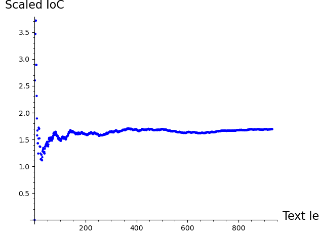
Experiment 2: IoC Convergence as Text Length Grows#
We study how the IoC stabilizes as the sample size increases. SageMath’s list_plot provides a convenient way to visualize this.
sample = '''This is the model used by many trade magazines (industry-based periodicals) distributed only to qualifying readers, often for free and determined by some form of survey. Because of costs (e.g., printing and postage) associated with the medium of print, publishers may not distribute free copies to everyone who requests one (unqualified leads); instead, they operate under controlled circulation, deciding who may receive free subscriptions based on each person's qualification as a member of the trade (and likelihood of buying, for example, likelihood of having corporate purchasing authority, as determined from job title). This allows a high level of certainty that advertisements will be received by the advertiser's target audience,[5] and it avoids wasted printing and distribution expenses. This latter model was widely used before the rise of the World Wide Web and is still employed by some titles. For example, in the United Kingdom, a number of computer-industry magazines use this model, including Computer Weekly and Computing, and in finance, Waters Magazine. For the global media industry, an example would be VideoAge International.'''
list_plot([IC(sample[0:k], lalphabet) for k in range(5, len(lclear(sample)))],
          axes_labels=['Text length', 'Scaled IoC'])
list_plot([IC(plaintext[0:k], lalphabet) for k in range(5, len(plaintext))],
          axes_labels=['Text length', 'Scaled IoC'])
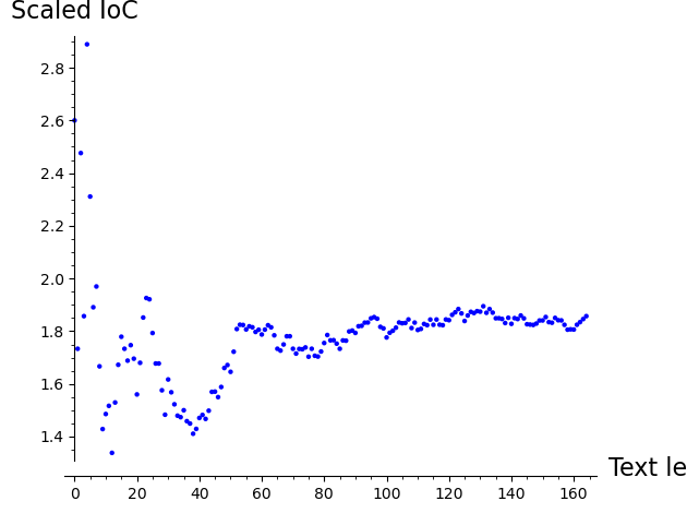
Observation
The IoC is noisy for short texts (fewer than about 50 characters) but quickly stabilizes. English text converges toward the scaled \(\kappa_p \approx 1.73\), while ciphertext and random text converge toward \(\kappa_r \approx 1.0\). This means the IoC method becomes reliable with as few as 100–200 characters.
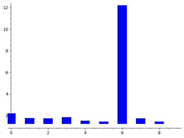
Experiment 3: IoC vs. Trial Key Length (Column Method)#
For each candidate key length \(L\), we extract every \(L\)-th character and compute the IoC. The correct \(L\) produces a peak near \(\kappa_p\).
a = 0
k = 3
N = len('123456789')

''.join(['123456789'[k*i+a] for i in range(0, N//k)])
'147'
# Compute column IoC for trial key lengths 1 through 9
a = 0
N = len(ciphertext)

([IC(''.join([ciphertext[kk*i] for i in range(0, N//kk)]), lalphabet) for kk in range(1, 10)])
[1.053393665158371,
 1.369187675070028,
 1.1987012987012986,
 1.9628339140534263,
 0.9269162210338681,
 1.5132275132275133,
 0.47101449275362317,
 1.361904761904762,
 0.6797385620915033]
Observation
The bar chart shows a clear peak at \(L = 6\) (the true key length for “enigma”). At the correct key length, the average column IoC is near \(\kappa_p\) (scaled \(\approx 1.73\)), confirming that each column is governed by a single Caesar shift. For wrong key lengths, the IoC hovers closer to \(\kappa_r\) (scaled \(\approx 1.0\)).
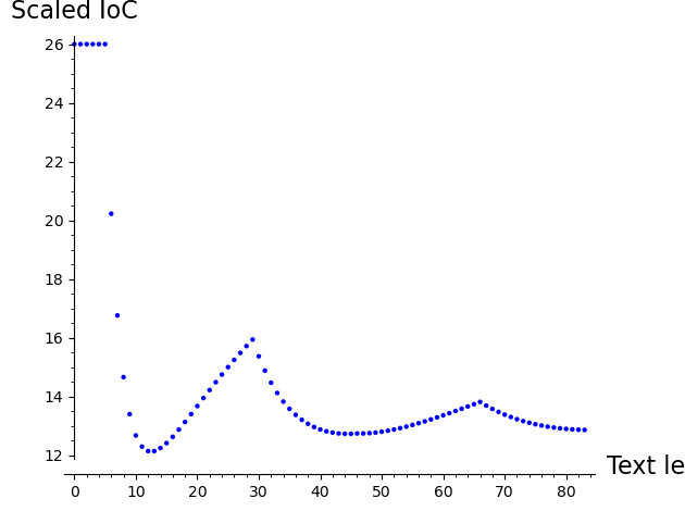
Experiment 4: Synthetic Example#
One can apply the index of coincidence to a synthetic example. Notice how differently the index stabilizes as we expand our context. How would you explain it?
# Synthetic example with very non-uniform plaintext
plaintext2 = lclear("aaaaaaaabbbbbbbbaaaaaaaaaaaaaaaabbbbbbbbbbbbbbbbbaaaaaaaaaaaaaaaaaaaabbbbbbbbbbbbbbbbbb")
key2 = "confuse"
ciphertext2 = vigenere_encrypt(plaintext2, key2)
print(ciphertext2)

decrypted_plaintext2 = vigenere_decrypt(ciphertext2, key2)
print(decrypted_plaintext2)
confusecpogvtfdpnfuseconfuseconfvtfdpogvtfdpogvtfconfuseconfuseconfusfdpogvtfdpogvtfdpo
aaaaaaaabbbbbbbbaaaaaaaaaaaaaaaabbbbbbbbbbbbbbbbbaaaaaaaaaaaaaaaaaaaabbbbbbbbbbbbbbbbbb
list_plot([IC(plaintext2[0:k], lalphabet) for k in range(3, len(lclear(plaintext2)))],
          axes_labels=['Text length', 'Scaled IoC'])
# Visualize column IoC with SageMath bar_chart
N = len(ciphertext2)
bar_chart([IC(''.join([ciphertext2[kk*i] for i in range(0, N//kk)]), lalphabet)
           for kk in range(1, 10)])
6.5 Kasiski Method with Substring Distance Analysis#
Kasiski examination, also known as Kasiski’s test or Kasiski’s method, is a technique used in cryptanalysis to break polyalphabetic substitution ciphers, such as the Vigenere cipher. It was initially introduced by Friedrich Kasiski in 1863, although Charles Babbage may have independently discovered it as early as 1846.
The key idea is to find repeated substrings in the ciphertext, compute the distances between their occurrences, and then factorize those distances. The key length should divide most of these distances, so the most common prime factor reveals the key length. SageMath’s gcd(), factor(), and ZZ.prime_factors() are natural tools for this analysis.
def find_substring_distance(s, n):
    """
    Finds the distance between identical substrings of length n in a given string.
    Returns -1 if no such substring is found.

    Args:
    s (str): The input string
    n (int): The length of the substring

    Returns:
    int: The distance between identical substrings of length n, or -1 if no such substring is found.
    """
    substring_indices = {}
    for i in range(len(s) - n + 1):
        substring = s[i:i+n]
        if substring in substring_indices:
            return i - substring_indices[substring]
        else:
            substring_indices[substring] = i
    return -1
s = "abc1243654364872364782346823abcfkdjfkdjfdkabc"
n = 3
distance = find_substring_distance(s, n)
print(distance)  # Output: 25
4
plaintext = lclear("hello world this is a short text to encrypt and decipher. Notice that this is done in pure english. We write and we send, this is our missions. Vignere cipher is safe, so they say. However, I am not so sure anymore, is it?")
key = "enigma"
ciphertext = vigenere_encrypt(plaintext, key)
[[find_substring_distance(ciphertext, k), k] for k in range(2, 10)]
[[42, 2], [108, 3], [-1, 4], [-1, 5], [-1, 6], [-1, 7], [-1, 8], [-1, 9]]
find_substring_distance('FGXTHJAQWNFGXQ', 3)
10
Experiment 5: Kasiski Examination with Key Length 4#
We encrypt the same plaintext with a 4-letter key and investigate the repeated trigram structure.
key2 = "abcd"
ciphertext2 = vigenere_encrypt(plaintext, key2)

[[find_substring_distance(ciphertext2, k), k] for k in range(2, 20)]
[[4, 2],
 [20, 3],
 [-1, 4],
 [-1, 5],
 [-1, 6],
 [-1, 7],
 [-1, 8],
 [-1, 9],
 [-1, 10],
 [-1, 11],
 [-1, 12],
 [-1, 13],
 [-1, 14],
 [-1, 15],
 [-1, 16],
 [-1, 17],
 [-1, 18],
 [-1, 19]]
trips = [ciphertext2[i:i+3] for i in range(0, len(ciphertext2)-3)]
tripsd = {i: ciphertext2[i:i+3] for i in range(0, len(ciphertext2)-3)}
set([(x, trips.count(x)) for x in trips if trips.count(x) > 1])
{('juv', 2), ('kvi', 2), ('prt', 2)}
[k for k in tripsd.keys() if tripsd[k] == 'prt']
[46, 150]
150-46
104
[k for k in tripsd.keys() if tripsd[k] == 'kvi']
[58, 166]
166-58
108
[k for k in tripsd.keys() if tripsd[k] == 'juv']
[105, 125]
125-105
20
# SageMath built-in gcd
gcd(104, 108)
4
Experiment 6: Kasiski with Key Length 5#
key3 = "abcde"
ciphertext3 = vigenere_encrypt(plaintext, key3)

[[find_substring_distance(ciphertext3, k), k] for k in range(2, 20)]
[[30, 2],
 [85, 3],
 [85, 4],
 [85, 5],
 [85, 6],
 [85, 7],
 [-1, 8],
 [-1, 9],
 [-1, 10],
 [-1, 11],
 [-1, 12],
 [-1, 13],
 [-1, 14],
 [-1, 15],
 [-1, 16],
 [-1, 17],
 [-1, 18],
 [-1, 19]]
trips3 = [ciphertext3[i:i+3] for i in range(0, len(ciphertext3)-3)]
tripsd3 = {i: ciphertext3[i:i+3] for i in range(0, len(ciphertext3)-3)}
tt3 = set([(x, trips3.count(x)) for x in trips3 if trips3.count(x) > 1])
tt3
{('hti', 2), ('ikv', 2), ('itu', 2), ('kvm', 2), ('tik', 2), ('vms', 2)}
[[[k for k in tripsd3.keys() if tripsd3[k] == f[0]], f[0]] for f in tt3]
[[[13, 98], 'vms'],
 [[12, 97], 'kvm'],
 [[105, 125], 'itu'],
 [[10, 95], 'tik'],
 [[9, 94], 'hti'],
 [[11, 96], 'ikv']]
[98-13, 125-105, 96-11, 94-9, 97-12, 95-10]
[85, 20, 85, 85, 85, 85]
gcd(85, 20)
5
Experiment 7: Kasiski with Key Length 7#
With a 7-letter key, we use both trigrams and digrams to gather more distance data. SageMath’s ZZ(...).prime_factors() and .factor() give direct access to prime factorizations.
key4 = "richard"  # seven letters
ciphertext4 = vigenere_encrypt(plaintext, key4)

[[find_substring_distance(ciphertext4, k), k] for k in range(2, 20)]
[[8, 2],
 [154, 3],
 [-1, 4],
 [-1, 5],
 [-1, 6],
 [-1, 7],
 [-1, 8],
 [-1, 9],
 [-1, 10],
 [-1, 11],
 [-1, 12],
 [-1, 13],
 [-1, 14],
 [-1, 15],
 [-1, 16],
 [-1, 17],
 [-1, 18],
 [-1, 19]]
trips4 = [ciphertext4[i:i+3] for i in range(0, len(ciphertext4)-3)]
tripsd4 = {i: ciphertext4[i:i+3] for i in range(0, len(ciphertext4)-3)}
tt4 = set([(x, trips4.count(x)) for x in trips4 if trips4.count(x) > 1])
tt4
{('zvz', 2)}
[[[k for k in tripsd4.keys() if tripsd4[k] == f[0]], f[0]] for f in tt4]
[[[12, 166], 'zvz']]
# SageMath factor() -- gives complete prime factorization
(166 - 12).factor()
2 * 7 * 11
doubles4 = [ciphertext4[i:i+2] for i in range(0, len(ciphertext4)-2)]
doublesd4 = {i: ciphertext4[i:i+2] for i in range(0, len(ciphertext4)-2)}
dd4 = set([(x, doubles4.count(x)) for x in doubles4 if doubles4.count(x) > 1])
dd4
{('ac', 2),
 ('ah', 2),
 ('ei', 2),
 ('et', 2),
 ('fa', 2),
 ('gf', 2),
 ('gp', 2),
 ('il', 2),
 ('kp', 2),
 ('lj', 3),
 ('oe', 2),
 ('pg', 2),
 ('pk', 2),
 ('rv', 2),
 ('vf', 2),
 ('vu', 2),
 ('vv', 2),
 ('vz', 2),
 ('wy', 2),
 ('ye', 2),
 ('yl', 3),
 ('za', 2),
 ('zi', 2),
 ('zv', 2)}
outs = [[[k for k in doublesd4.keys() if doublesd4[k] == f[0]], f[0]] for f in dd4]
outs
[[[27, 35], 'rv'],
 [[14, 105], 'za'],
 [[76, 97, 125], 'lj'],
 [[28, 144], 'vv'],
 [[12, 166], 'zv'],
 [[56, 133], 'kp'],
 [[59, 147], 'zi'],
 [[10, 52], 'ah'],
 [[82, 124], 'il'],
 [[36, 153], 'vf'],
 [[42, 65], 'gp'],
 [[13, 167], 'vz'],
 [[43, 134], 'pg'],
 [[24, 39], 'et'],
 [[9, 154], 'fa'],
 [[79, 96, 142], 'yl'],
 [[57, 93], 'pk'],
 [[109, 122], 'oe'],
 [[15, 127], 'ac'],
 [[62, 135], 'gf'],
 [[101, 145], 'vu'],
 [[116, 123], 'ei'],
 [[141, 156], 'wy'],
 [[157, 164], 'ye']]
# SageMath ZZ(...).prime_factors() -- returns list of prime divisors
pr = [ZZ(x[0][1] - x[0][0]).prime_factors() for x in outs]
pr
[[2],
 [7, 13],
 [3, 7],
 [2, 29],
 [2, 7, 11],
 [7, 11],
 [2, 11],
 [2, 3, 7],
 [2, 3, 7],
 [3, 13],
 [23],
 [2, 7, 11],
 [7, 13],
 [3, 5],
 [5, 29],
 [17],
 [2, 3],
 [13],
 [2, 7],
 [73],
 [2, 11],
 [7],
 [3, 5],
 [7]]
# Tally the prime factors to find the most common one
pprep = []
for el in pr:
    pprep += el
[[x, pprep.count(x)] for x in sorted(list(set(pprep)))]
[[2, 10],
 [3, 7],
 [5, 3],
 [7, 11],
 [11, 5],
 [13, 4],
 [17, 1],
 [23, 1],
 [29, 2],
 [73, 1]]
6.6 A Complete Attack on the Vigenere Cipher#
So now let us apply the Kasiski method to finally perform a full attack on the Vigenere cipher. We will:
Use repeated n-gram distances and prime factorization to determine the key length
Apply frequency analysis to each column to recover the individual key letters
The attack pipeline
The complete Vigenere attack consists of two distinct phases:
Key length determination using the Index of Coincidence (column method) or the Kasiski examination (distance factorization).
Key recovery using frequency analysis on each column. Once the key length \(L\) is known, the problem reduces to \(L\) independent Caesar ciphers.
poem = '''Ciphers, oh ciphers, secrets they keep
Locked away in code, deep and discreet
Symbols and numbers, jumbled and mixed
A message encoded, ready to be fixed

Through history they've been used to hide
Plans of war, love letters beside
The Rosetta Stone, a mystery solved
A codebreaker's work, duly evolved

From Caesar to Enigma, through time they change
Yet the essence remains, mysterious and strange
A puzzle to solve, a game to play
A message to decipher, in every way

Crack the code, reveal the truth
A challenge to minds, sharp and astute
For ciphers, oh ciphers, they hold the key
To secrets untold, waiting to be set free.'''
plaintext = lclear(poem)

key5 = "hunter"  # six letters
ciphertext5 = vigenere_encrypt(plaintext, key5)

print([[find_substring_distance(ciphertext5, k), k] for k in range(2, 20)])

trips5 = [ciphertext5[i:i+3] for i in range(0, len(ciphertext5)-3)]
tripsd5 = {i: ciphertext5[i:i+3] for i in range(0, len(ciphertext5)-3)}
tt5 = set([(x, trips5.count(x)) for x in trips5 if trips5.count(x) > 1])
tt5
[[12, 2], [18, 3], [114, 4], [348, 5], [348, 6], [-1, 7], [-1, 8], [-1, 9], [-1, 10], [-1, 11], [-1, 12], [-1, 13], [-1, 14], [-1, 15], [-1, 16], [-1, 17], [-1, 18], [-1, 19]]
{('abr', 2),
 ('bli', 2),
 ('brv', 2),
 ('ekm', 2),
 ('goy', 2),
 ('gyh', 2),
 ('iiz', 2),
 ('ika', 2),
 ('koy', 3),
 ('lik', 2),
 ('lll', 2),
 ('lnb', 2),
 ('mgo', 2),
 ('nux', 3),
 ('oye', 2),
 ('oyl', 3),
 ('rms', 2),
 ('sul', 2),
 ('tru', 2),
 ('vmg', 2),
 ('wko', 2),
 ('yel', 3)}
outs5 = [[[k for k in tripsd5.keys() if tripsd5[k] == f[0]], f[0]] for f in tt5]
outs5
[[[4, 76], 'iiz'],
 [[274, 400], 'gyh'],
 [[311, 413], 'ekm'],
 [[11, 359], 'goy'],
 [[283, 391, 457], 'nux'],
 [[188, 464], 'bli'],
 [[10, 358], 'mgo'],
 [[24, 138, 450], 'oyl'],
 [[13, 175, 223], 'yel'],
 [[270, 378], 'abr'],
 [[22, 448], 'wko'],
 [[12, 360], 'oye'],
 [[342, 382], 'sul'],
 [[263, 408], 'lnb'],
 [[23, 137, 449], 'koy'],
 [[172, 190], 'ika'],
 [[9, 357], 'vmg'],
 [[326, 338], 'rms'],
 [[363, 379], 'brv'],
 [[189, 489], 'lik'],
 [[204, 205], 'lll'],
 [[51, 69], 'tru']]
# Prime factorization of trigram distances
[ZZ(x[0][1] - x[0][0]).prime_factors() for x in outs5]
[[2, 3],
 [2, 3, 7],
 [2, 3, 17],
 [2, 3, 29],
 [2, 3],
 [2, 3, 23],
 [2, 3, 29],
 [2, 3, 19],
 [2, 3],
 [2, 3],
 [2, 3, 71],
 [2, 3, 29],
 [2, 5],
 [5, 29],
 [2, 3, 19],
 [2, 3],
 [2, 3, 29],
 [2, 3],
 [2],
 [2, 3, 5],
 [],
 [2, 3]]
doubles5 = [ciphertext5[i:i+2] for i in range(0, len(ciphertext5)-2)]
doublesd5 = {i: ciphertext5[i:i+2] for i in range(0, len(ciphertext5)-2)}
dd5 = set([(x, doubles5.count(x)) for x in doubles5 if doubles5.count(x) > 1])
print(dd5)
{('yw', 2), ('zi', 2), ('yl', 4), ('vk', 5), ('ck', 2), ('vo', 2), ('jt', 3), ('fr', 2), ('vc', 2), ('ik', 4), ('tv', 2), ('mf', 2), ('hh', 2), ('hf', 2), ('rr', 3), ('kc', 2), ('vy', 2), ('ba', 3), ('pr', 2), ('kv', 4), ('we', 3), ('li', 4), ('go', 2), ('iv', 2), ('yq', 3), ('uk', 2), ('wv', 3), ('th', 2), ('cy', 2), ('wb', 2), ('gb', 2), ('su', 2), ('ek', 2), ('dh', 2), ('ya', 3), ('ov', 2), ('ye', 7), ('rw', 2), ('ir', 2), ('jz', 2), ('va', 2), ('cc', 2), ('lr', 4), ('ru', 2), ('yh', 2), ('tr', 3), ('ai', 3), ('oi', 2), ('mg', 3), ('ka', 2), ('ar', 2), ('vf', 3), ('gf', 2), ('nb', 6), ('ly', 3), ('iz', 2), ('iy', 2), ('ee', 2), ('ft', 3), ('ii', 4), ('il', 2), ('el', 4), ('km', 3), ('rm', 3), ('oy', 5), ('ff', 2), ('tg', 3), ('nu', 5), ('ko', 3), ('kl', 2), ('ze', 2), ('hp', 2), ('vm', 2), ('xx', 2), ('ll', 5), ('ei', 2), ('fv', 2), ('vz', 3), ('fm', 3), ('sc', 2), ('gy', 2), ('qt', 2), ('xr', 2), ('la', 2), ('ux', 3), ('qv', 2), ('ul', 4), ('jv', 2), ('sl', 2), ('ln', 3), ('cv', 2), ('wk', 3), ('br', 5), ('iu', 2), ('bl', 2), ('ms', 3), ('rj', 2), ('ml', 2), ('rv', 3), ('ab', 3), ('xj', 2), ('vv', 3), ('fy', 3), ('vi', 2), ('bk', 2), ('an', 2), ('kn', 2), ('xi', 2), ('zu', 2), ('gk', 2), ('vl', 2)}
outs52 = [[[k
for k in doublesd5.keys()
if doublesd5[k] == f[0]], f[0]]
for f in dd5]
pr5 = [ZZ(x[0][1] - x[0][0]).prime_factors() for x in outs52]
print(pr5)
[[2, 11], [3, 5, 23], [2, 3, 19], [2, 3], [11, 29], [3, 31], [2, 3, 7], [263], [199], [2, 3], [2, 3, 7], [2, 3, 53], [3, 19], [2, 7, 23], [2, 5, 13], [3], [5, 37], [3, 5], [79], [151], [2, 5, 7], [5, 13], [2, 3, 29], [97], [2, 3, 5], [3, 23], [2, 3, 11], [2, 67], [2, 3, 13], [401], [2, 5, 11], [2, 5], [2, 3, 17], [2, 89], [2, 3], [2, 3, 71], [2, 3], [109], [2, 3, 7], [13], [2, 3], [2, 13], [2, 3, 5], [2, 3], [2, 3, 7], [2, 3], [3, 37], [2, 3, 41], [3, 101], [2, 3], [2, 3], [2, 3, 11], [2, 5, 11], [2, 3], [2, 3], [2, 3], [2, 7, 11], [2, 3], [2, 3, 5], [2, 3], [2, 71], [2, 3], [2, 3, 17], [2, 3, 17], [2, 3], [2, 7], [2, 3], [2, 3], [2, 3, 19], [5, 19], [2, 61], [3], [2, 3, 29], [2, 3, 5, 7], [2, 3], [13, 19], [2, 61], [17], [2, 3], [2, 3, 41], [2, 3, 7], [2], [2, 5], [227], [2, 3], [2, 3, 13], [2, 3], [2, 3, 7], [7, 17], [7, 29], [113], [2, 3, 5], [2, 13], [3, 13], [2, 3, 23], [2, 3, 11], [2, 3, 23], [3, 41], [2], [2], [2, 3, 13], [], [2, 11], [11, 13], [11], [2, 17], [2, 3, 17], [109], [3, 11], [13], [2, 3, 7]]
# Tally the prime factors
pprep = []
for el in pr5:
    pprep += el
[[x, pprep.count(x)] for x in sorted(list(set(pprep)))]
[[2, 76],
 [3, 66],
 [5, 16],
 [7, 14],
 [11, 12],
 [13, 12],
 [17, 7],
 [19, 5],
 [23, 5],
 [29, 4],
 [31, 1],
 [37, 2],
 [41, 3],
 [53, 1],
 [61, 2],
 [67, 1],
 [71, 2],
 [79, 1],
 [89, 1],
 [97, 1],
 [101, 1],
 [109, 2],
 [113, 1],
 [151, 1],
 [199, 1],
 [227, 1],
 [263, 1],
 [401, 1]]
Observation
The most common prime factors in the distances are 2 and 3, and their product \(2 \times 3 = 6\) appears frequently. This strongly suggests the key length is 6.
Applying Frequency Analysis to Find the Letters of the Key#
Once we have established the key length, we can apply frequency analysis to find the exact key. Each column of the ciphertext (characters at positions \(0, 6, 12, \ldots\); then \(1, 7, 13, \ldots\); etc.) was encrypted with a single Caesar shift. The most frequent letter in each column should correspond to ‘e’ (the most common English letter).
letlist = [[ciphertext5[6*i + k] for i in range(len(ciphertext5)//6 - 1)] for k in range(6)]
sorted([[letlist[0].count(x), x] for x in list(set(letlist[0]))])
[[1, 'b'],
 [1, 'e'],
 [1, 'g'],
 [1, 'r'],
 [1, 't'],
 [2, 'c'],
 [2, 'f'],
 [2, 'j'],
 [2, 'n'],
 [2, 's'],
 [2, 'u'],
 [3, 'p'],
 [3, 'w'],
 [4, 'y'],
 [5, 'h'],
 [5, 'o'],
 [6, 'z'],
 [7, 'v'],
 [8, 'a'],
 [9, 'k'],
 [14, 'l']]
# If the most frequent letter in column 0 is 'l', and we expect 'e':
ord('l') - ord('e')  # shift = 7, which is 'h'
7
# Verify: the first letter of "hunter" is 'h'
ord('h') - ord('a')
7
def Frequency(text, alphabet):
    """Compute relative letter frequencies."""
    s = lclear(text)
    return [float(s.count(let) / len(s)) for let in alphabet]


textsample = '''Deep within the caves so dark and cold,
The dwarves, they sat and stories told,
Of treasure hoards and ancient lore,
And secrets kept for evermore.

But in their hands they held a tool,
A wondrous thing, so sharp and cool,
A blade of steel that could carve letters,
And keep their secrets safe forever.

They used this tool to write their code,
A cipher strong that none could decode,
For every letter they would add,
Another from their secret pad.

The Vigenere cipher was their art,
A thing of beauty, a thing apart,
For only those who held the key,
Could read the messages meant to be.

And so they wrote, in cryptic lines,
Their secrets safe from prying eyes,
For only those who knew the code,
Could ever hope to share the load.

And though the world may never know,
The secrets kept so long ago,
The dwarves will always have their craft,
The Vigenere cipher, strong and steadfast.
'''

import string
import re
latin_alphabet = list(string.ascii_lowercase)

list(reversed(sorted(list(zip(Frequency(textsample, latin_alphabet), latin_alphabet)))))[0:5]
[(0.15195369030390737, 'e'),
 (0.10274963820549927, 't'),
 (0.0824891461649783, 'o'),
 (0.08104196816208394, 'r'),
 (0.07525325615050651, 'a')]
Recovering Each Key Letter#
For each of the 6 columns, we find the most frequent letter and deduce the key letter by assuming it maps from ‘e’.
# Column 0
list(reversed(sorted([[letlist[0].count(x), x] for x in list(set(letlist[0]))])))[0:2]
[[14, 'l'], [9, 'k']]
chr(97 + ord('l') - ord('e')) # key letter 0: 'h'
'h'
# Column 1
list(reversed(sorted([[letlist[1].count(x), x] for x in list(set(letlist[1]))])))[0:2]
[[18, 'y'], [11, 'n']]
chr(97 + ord('y') - ord('e')) # key letter 1: 'u'
'u'
# Column 2
list(reversed(sorted([[letlist[2].count(x), x] for x in list(set(letlist[2]))])))[0:2]
[[11, 'r'], [9, 'b']]
chr(97 + ord('r') - ord('e')) # key letter 2: 'n'
'n'
# Column 3
list(reversed(sorted([[letlist[3].count(x), x] for x in list(set(letlist[3]))])))[0:2]
[[12, 't'], [9, 'x']]
chr(97 + ord('x') - ord('e')) # key letter 3: 't'
't'
# Column 4
list(reversed(sorted([[letlist[4].count(x), x] for x in list(set(letlist[4]))])))[0:2]
[[14, 'i'], [7, 's']]
chr(97 + ord('i') - ord('e')) # key letter 4: 'e'
'e'
# Column 5
list(reversed(sorted([[letlist[5].count(x), x] for x in list(set(letlist[5]))])))[0:2]
[[15, 'v'], [9, 'k']]
chr(97 + ord('v') - ord('e')) # key letter 5: 'r'
'r'
Result
The recovered key is “hunter”, which matches the true key exactly! The full attack pipeline:
Kasiski/IoC analysis determined the key length is 6
Frequency analysis on each of the 6 columns recovered each key letter
The ciphertext can now be fully decrypted
# Decrypt and verify
recovered_key = "hunter"
decrypted = vigenere_decrypt(ciphertext5, recovered_key)
print("Recovered key:", recovered_key)
print("Decrypted text:")
print(decrypted)
Recovered key: hunter
Decrypted text:
ciphersohcipherssecretstheykeeplockedawayincodedeepanddiscreetsymbolsandnumbersjumbledandmixedamessageencodedreadytobefixedthroughhistorytheyvebeenusedtohideplansofwarlovelettersbesidetherosettastoneamysterysolvedacodebreakersworkdulyevolvedfromcaesartoenigmathroughtimetheychangeyettheessenceremainsmysteriousandstrangeapuzzletosolveagametoplayamessagetodecipherineverywaycrackthecoderevealthetruthachallengetomindssharpandastuteforciphersohcipherstheyholdthekeytosecretsuntoldwaitingtobesetfree
Exercises#
Exercise 6.1: IoC for different languages
The letter frequency distributions differ across languages. The following table gives approximate \(\kappa_p\) values for several languages:
Language |
\(\kappa_p\) |
|---|---|
English |
0.0667 |
French |
0.0778 |
German |
0.0762 |
Italian |
0.0738 |
Spanish |
0.0775 |
Russian |
0.0529 |
(a) Explain why Russian has a lower \(\kappa_p\) than the other languages listed. (Hint: consider the alphabet size.)
(b) Using the French frequency distribution below, compute \(\kappa_p\) for French and verify it is approximately 0.0778.
# French letter frequencies (A-Z)
french_freq = [
    0.0815, 0.0097, 0.0315, 0.0373, 0.1739, 0.0112,
    0.0097, 0.0085, 0.0731, 0.0045, 0.0002, 0.0546,
    0.0296, 0.0712, 0.0528, 0.0303, 0.0099, 0.0655,
    0.0808, 0.0707, 0.0574, 0.0132, 0.0004, 0.0045,
    0.0030, 0.0012
]
kappa_p_french = sum(p^2 for p in french_freq)
print(f"kappa_p for French: {kappa_p_french:.4f}")
(c) How would Friedman’s key length formula change for a French-language ciphertext?
Exercise 6.2: Proving IoC invariance
Prove that the Index of Coincidence is invariant under any monoalphabetic substitution cipher. That is, if \(\sigma: \mathcal{A} \to \mathcal{A}\) is a bijection and \(y = \sigma(x_1)\sigma(x_2)\cdots\sigma(x_N)\), then \(\mathrm{IC}(y) = \mathrm{IC}(x)\).
Hint: A bijection \(\sigma\) merely permutes the frequency counts \(\{f_0, f_1, \ldots, f_{25}\}\), but the IoC formula is a symmetric function of these counts.
Exercise 6.3: Implementing Friedman’s key length formula in SageMath
Write a SageMath function friedman_estimate(ciphertext) that:
Computes the observed IoC of the ciphertext.
Applies the formula \(L \approx (\kappa_p - \kappa_r) / (\mathrm{IC}_{\text{obs}} - \kappa_r)\).
Returns the nearest integer as the estimated key length.
Test your function on the ciphertext produced by encrypting the text "the quick brown fox jumps over the lazy dog" repeated 20 times with the keys "ab", "code", "secret", and "cryptanalysis". Compare the estimates with the true key lengths.
Hint: Use SageMath’s round() for rounding to the nearest integer.
Exercise 6.4: Automated Vigenere attack
Write a complete SageMath function break_vigenere(ciphertext, max_key_length=20) that:
Uses the IoC column method to determine the key length.
Uses frequency analysis to recover each key letter.
Returns the recovered key and the decrypted plaintext.
Test your function by encrypting a paragraph from a book with a key of your choice, then verify that your function recovers the correct key.
Hint: Use SageMath’s bar_chart() or list_plot() to visualize the column IoC values as part of your analysis.
Exercise 6.5: Combining Kasiski and IoC
Apply both the Kasiski method and the IoC column method to the same ciphertext. Do they agree on the key length? Under what circumstances might they disagree?
Hint: Use ZZ(...).prime_factors() for the Kasiski analysis and bar_chart() for the IoC visualization.
Summary#
In this chapter we introduced the Index of Coincidence, a statistical tool invented by William F. Friedman that revolutionized the cryptanalysis of polyalphabetic ciphers. We combined it with the Kasiski examination to perform a complete attack on the Vigenere cipher.
Key concepts:
Index of Coincidence (IoC): The probability that two randomly chosen letters from a text are the same: \(\mathrm{IC}(x) = \sum f_i(f_i - 1) / N(N-1)\).
Benchmark values: English text has \(\kappa_p \approx 0.0667\); uniformly random text has \(\kappa_r = 1/26 \approx 0.0385\).
Invariance: The IoC is invariant under monoalphabetic substitution (any permutation of the alphabet).
Friedman’s Theorem: For a polyalphabetic cipher with key length \(L\), the expected IoC is \(\mathrm{IC} \approx (\kappa_p - \kappa_r)/L + \kappa_r\).
Key length estimation: The column method splits ciphertext into \(L\) columns and checks whether the average column IoC is close to \(\kappa_p\). Peaks at the correct \(L\) and its multiples.
Kasiski examination: Finding repeated n-grams and factorizing their distances with
ZZ(...).prime_factors()andgcd()to determine the key length.Full attack: Once the key length is known, frequency analysis on each column recovers the individual key letters.
SageMath tools used: gcd(), factor(), ZZ.prime_factors(), list_plot(), bar_chart() – no NumPy or matplotlib needed.
References#
Friedman, W. F. (1922). The Index of Coincidence and Its Applications in Cryptanalysis. Riverbank Publication No. 22. Department of Ciphers, Riverbank Laboratories, Geneva, Illinois. [1]
Kasiski, F. W. (1863). Die Geheimschriften und die Dechiffrir-Kunst. Berlin: E. S. Mittler und Sohn. [2]
Sinkov, A. (1966). Elementary Cryptanalysis: A Mathematical Approach. Mathematical Association of America. – Chapters 4-5 provide an accessible introduction to the IoC and Kasiski methods.
Bauer, F. L. (2007). Decrypted Secrets: Methods and Maxims of Cryptology. 4th edition, Springer. – Chapter 3 gives a thorough treatment of polyalphabetic ciphers and the IoC.
Singh, S. (1999). The Code Book: The Science of Secrecy from Ancient Egypt to Quantum Cryptography. Doubleday. [3] – Chapter 2 tells the story of Friedman and the breaking of polyalphabetic ciphers.
Kahn, D. (1996). The Codebreakers: The Comprehensive History of Secret Communication from Ancient Times to the Internet. Revised edition, Scribner. – Chapters 12-13 cover Friedman’s contributions in detail.