
Chapter 37: Quantum Computing Foundations for Cryptanalysis#
“Nature isn’t classical, dammit, and if you want to make a simulation of nature, you’d better make it quantum mechanical.” — Richard Feynman, 1981
“Quantum mechanics is not just about small things. It is simply the way the world works.” — David Deutsch, 1997
This chapter introduces the mathematical foundations of quantum computing that are essential for understanding Shor’s algorithm (Chapter 38) and Grover’s algorithm (Chapter 39). We build the concepts from scratch: qubits, quantum gates, measurement, entanglement, and simple quantum circuits. No prior knowledge of quantum mechanics is assumed — only linear algebra over \(\mathbb{C}\).
37.1 Historical Context#
The path from classical to quantum computation was paved by a series of landmark theoretical advances over roughly fifteen years:
Key Milestones Leading to Shor’s Algorithm
Year |
Contributor |
Contribution |
|---|---|---|
1981 |
Feynman |
Proposed that quantum systems could simulate physics exponentially faster than classical computers |
1985 |
Deutsch |
Formalized the quantum Turing machine, showing that quantum mechanics permits a universal model of computation |
1992 |
Deutsch & Jozsa |
First quantum algorithm with provable speedup: distinguishes constant from balanced Boolean functions in one query |
1993 |
Bernstein & Vazirani |
Extended Deutsch–Jozsa; showed quantum query complexity can be exponentially smaller than classical |
1994 |
Simon |
Oracle problem with exponential quantum speedup, directly inspiring Shor’s period-finding approach |
1994 |
Shor |
Polynomial-time quantum algorithms for factoring and discrete logarithms — the event that launched post-quantum cryptography |
Each of these milestones built on the previous one. Deutsch showed quantum computation was possible; Deutsch–Jozsa and Bernstein–Vazirani demonstrated quantum speedups for oracle problems; Simon found an exponential oracle separation using periodicity; and Shor realized that period finding could be applied to a concrete number-theoretic problem — factoring — with devastating consequences for public-key cryptography.
Why Cryptanalysts Must Understand Quantum Computing
Shor’s algorithm does not merely weaken RSA and Diffie–Hellman — it breaks them completely in polynomial time. Understanding why requires grasping the quantum phenomena (superposition, interference, entanglement) that make this speedup possible. This chapter provides that foundation.
37.2 Formal Definitions#
Qubits and State Space#
Definition 37.1 — Qubit
A qubit is a quantum system whose state is a unit vector in \(\mathbb{C}^2\). Using Dirac notation, the computational basis states are
A general qubit state is a superposition:
where \(\alpha, \beta \in \mathbb{C}\) are called amplitudes.
Bloch sphere representation. Up to a global phase, any qubit state can be written as
where \(\theta \in [0, \pi]\) and \(\phi \in [0, 2\pi)\) are spherical coordinates on the Bloch sphere. The north pole is \(|0\rangle\), the south pole is \(|1\rangle\), and the equator contains states like \(|+\rangle = \frac{1}{\sqrt{2}}(|0\rangle + |1\rangle)\).
Definition 37.2 — Quantum Gates
A quantum gate on \(n\) qubits is a \(2^n \times 2^n\) unitary matrix \(U\) (satisfying \(U^\dagger U = I\)). The standard single-qubit gates are:
The key two-qubit gate is the CNOT (controlled-NOT):
which flips the target qubit if and only if the control qubit is \(|1\rangle\).
\(X\) is the quantum NOT gate (bit-flip).
\(Z\) is the phase-flip gate.
\(H\) (Hadamard) creates equal superpositions: \(H|0\rangle = |+\rangle\).
\(T\) is the \(\pi/8\)-gate, essential for universal quantum computation.
\(\{H, T, \text{CNOT}\}\) form a universal gate set: any unitary can be approximated to arbitrary precision.
Definition 37.3 — Measurement (Born Rule)
Projective measurement in the computational basis collapses the qubit state \(|\psi\rangle = \alpha|0\rangle + \beta|1\rangle\) to:
outcome \(0\) with probability \(|\alpha|^2\), post-measurement state \(|0\rangle\);
outcome \(1\) with probability \(|\beta|^2\), post-measurement state \(|1\rangle\).
This is the Born rule. Measurement is irreversible — it destroys the superposition. For an \(n\)-qubit state \(|\psi\rangle = \sum_{x=0}^{2^n-1} \alpha_x |x\rangle\), measuring all qubits gives outcome \(x\) with probability \(|\alpha_x|^2\).
Definition 37.4 — Tensor Product and Multi-Qubit States
The state space of \(n\) qubits is the tensor product \(\mathbb{C}^2 \otimes \cdots \otimes \mathbb{C}^2 = \mathbb{C}^{2^n}\).
If qubit 1 is in state \(|\psi_1\rangle\) and qubit 2 is in state \(|\psi_2\rangle\) (and they are unentangled), the combined state is
Concretely, if \(|\psi_1\rangle = (a, b)^T\) and \(|\psi_2\rangle = (c, d)^T\), then \(|\psi_1\rangle \otimes |\psi_2\rangle = (ac, ad, bc, bd)^T\).
Definition 37.5 — Quantum Entanglement (Bell States)
A multi-qubit state is entangled if it cannot be written as a tensor product of individual qubit states. The four Bell states are maximally entangled two-qubit states:
Measuring one qubit of \(|\Phi^+\rangle\) instantly determines the other: if qubit 1 is measured as \(|0\rangle\), qubit 2 must be \(|0\rangle\), and vice versa. This correlation holds regardless of the spatial separation of the qubits.
Theorem 37.1 — No-Cloning Theorem
There is no unitary operator \(U\) that can clone an arbitrary unknown quantum state. That is, there is no \(U\) such that
for all \(|\psi\rangle \in \mathbb{C}^2\).
Proof sketch. Suppose \(U\) clones two states \(|\psi\rangle\) and \(|\phi\rangle\):
Taking the inner product of both sides and using unitarity of \(U\):
This equation has only two solutions: \(\langle\psi|\phi\rangle = 0\) or \(\langle\psi|\phi\rangle = 1\). So \(U\) can only clone states that are identical or orthogonal — not arbitrary states. \(\square\)
Cryptographic Significance of No-Cloning
The no-cloning theorem is the foundation of quantum key distribution (QKD): an eavesdropper cannot copy quantum states in transit without disturbing them, making interception detectable. Ironically, the same quantum mechanics that threatens classical crypto via Shor’s algorithm also enables provably secure key exchange via QKD.
37.3 Implementation#
We implement a minimal quantum simulator from scratch using only numpy. This simulator will be reused in Chapters 38 and 39.
import numpy as np
import math

# ============================================================
# Standard gate matrices
# ============================================================

# Single-qubit gates
GATE_I = np.eye(2, dtype=complex)
GATE_X = np.array([[0, 1], [1, 0]], dtype=complex)
GATE_Y = np.array([[0, -1j], [1j, 0]], dtype=complex)
GATE_Z = np.array([[1, 0], [0, -1]], dtype=complex)
GATE_H = np.array([[1, 1], [1, -1]], dtype=complex) / np.sqrt(2)
GATE_S = np.array([[1, 0], [0, 1j]], dtype=complex)
GATE_T = np.array([[1, 0], [0, np.exp(1j * np.pi / 4)]], dtype=complex)

# Two-qubit gates
GATE_CNOT = np.array([
    [1, 0, 0, 0],
    [0, 1, 0, 0],
    [0, 0, 0, 1],
    [0, 0, 1, 0]
], dtype=complex)

GATE_SWAP = np.array([
    [1, 0, 0, 0],
    [0, 0, 1, 0],
    [0, 1, 0, 0],
    [0, 0, 0, 1]
], dtype=complex)


def rotation_z(theta):
    """Rz(theta) = diag(e^{-i*theta/2}, e^{i*theta/2})."""
    return np.array([
        [np.exp(-1j * theta / 2), 0],
        [0, np.exp(1j * theta / 2)]
    ], dtype=complex)


def rotation_y(theta):
    """Ry(theta) rotation about Y-axis."""
    c = np.cos(theta / 2)
    s = np.sin(theta / 2)
    return np.array([[c, -s], [s, c]], dtype=complex)


def rotation_x(theta):
    """Rx(theta) rotation about X-axis."""
    c = np.cos(theta / 2)
    s = np.sin(theta / 2)
    return np.array([[c, -1j * s], [-1j * s, c]], dtype=complex)


# --- Verify all gates are unitary ---
gates = {
    'I': GATE_I, 'X': GATE_X, 'Y': GATE_Y, 'Z': GATE_Z,
    'H': GATE_H, 'S': GATE_S, 'T': GATE_T,
    'CNOT': GATE_CNOT, 'SWAP': GATE_SWAP
}

print('Gate unitarity checks:')
for name, gate in gates.items():
    product = gate @ gate.conj().T
    is_unitary = np.allclose(product, np.eye(gate.shape[0]))
    print(f'  {name:>5}: {gate.shape[0]}x{gate.shape[0]}, '
          f'unitary = {is_unitary}')

# Show Hadamard action on |0> and |1>
ket0 = np.array([1, 0], dtype=complex)
ket1 = np.array([0, 1], dtype=complex)
print(f'\nH|0> = {GATE_H @ ket0}  (= |+>)')
print(f'H|1> = {GATE_H @ ket1}  (= |->)')
Gate unitarity checks:
      I: 2x2, unitary = True
      X: 2x2, unitary = True
      Y: 2x2, unitary = True
      Z: 2x2, unitary = True
      H: 2x2, unitary = True
      S: 2x2, unitary = True
      T: 2x2, unitary = True
   CNOT: 4x4, unitary = True
   SWAP: 4x4, unitary = True

H|0> = [0.70710678+0.j 0.70710678+0.j]  (= |+>)
H|1> = [ 0.70710678+0.j -0.70710678+0.j]  (= |->)
import numpy as np
import math


class Qubit:
    """Single-qubit quantum state simulator.

    Attributes
    ----------
    state : ndarray of shape (2,), complex
        The state vector [alpha, beta] with |alpha|^2 + |beta|^2 = 1.
    """

    def __init__(self, alpha=1.0, beta=0.0):
        self.state = np.array([alpha, beta], dtype=complex)
        self._normalize()

    def _normalize(self):
        norm = np.linalg.norm(self.state)
        if norm > 1e-15:
            self.state /= norm

    def apply_gate(self, gate):
        """Apply a 2x2 unitary gate to this qubit."""
        self.state = gate @ self.state
        self._normalize()
        return self

    def measure(self):
        """Perform projective measurement in computational basis.

        Returns 0 or 1 probabilistically (Born rule) and collapses state.
        """
        prob_0 = np.abs(self.state[0]) ** 2
        outcome = 0 if np.random.random() < prob_0 else 1
        self.state = np.array([1, 0], dtype=complex) if outcome == 0 \
            else np.array([0, 1], dtype=complex)
        return outcome

    def probabilities(self):
        """Return (prob_0, prob_1) without collapsing."""
        return np.abs(self.state[0])**2, np.abs(self.state[1])**2

    def bloch_coordinates(self):
        """Return (theta, phi) on the Bloch sphere.

        |psi> = cos(theta/2)|0> + e^{i*phi} sin(theta/2)|1>
        """
        alpha, beta = self.state
        theta = 2 * np.arccos(np.clip(np.abs(alpha), 0, 1))
        phi = np.angle(beta) - np.angle(alpha)
        return float(theta), float(phi)

    def bloch_xyz(self):
        """Return (x, y, z) Cartesian coords on Bloch sphere."""
        theta, phi = self.bloch_coordinates()
        x = np.sin(theta) * np.cos(phi)
        y = np.sin(theta) * np.sin(phi)
        z = np.cos(theta)
        return float(x), float(y), float(z)

    def copy(self):
        q = Qubit()
        q.state = self.state.copy()
        return q

    def __repr__(self):
        a, b = self.state
        return f'Qubit({float(a):.4f}|0> + {float(b):.4f}|1>)'


# --- Demo ---
q = Qubit()  # |0>
print(f'Initial state: {q}')
print(f'Bloch coords (theta, phi): {q.bloch_coordinates()}')
print(f'Bloch (x,y,z): {q.bloch_xyz()}  (north pole = |0>)')

H = np.array([[1, 1], [1, -1]], dtype=complex) / np.sqrt(2)
q.apply_gate(H)
print(f'\nAfter H: {q}')
print(f'Probabilities: {q.probabilities()}')
print(f'Bloch (x,y,z): {q.bloch_xyz()}  (equator = |+>)')
Initial state: Qubit(1.0000|0> + 0.0000|1>)
Bloch coords (theta, phi): (0.0, 0.0)
Bloch (x,y,z): (0.0, 0.0, 1.0)  (north pole = |0>)

After H: Qubit(0.7071|0> + 0.7071|1>)
Probabilities: (0.5000000000000001, 0.5000000000000001)
Bloch (x,y,z): (1.0, 0.0, 6.123233995736766e-17)  (equator = |+>)
/var/folders/z7/wp7m8p7x1250jzvklw5z24mm0000gn/T/ipykernel_75402/1727016520.py:69: ComplexWarning: Casting complex values to real discards the imaginary part
  return f'Qubit({float(a):.4f}|0> + {float(b):.4f}|1>)'
import numpy as np
import math


class QuantumRegister:
    """Multi-qubit quantum state simulator using full state vector.

    The state is stored as a complex vector of length 2^n.

    Parameters
    ----------
    n_qubits : int
        Number of qubits.
    """

    def __init__(self, n_qubits):
        self.n = n_qubits
        self.dim = 2 ** n_qubits
        self.state = np.zeros(self.dim, dtype=complex)
        self.state[0] = 1.0  # Initialize to |00...0>

    def _normalize(self):
        norm = np.linalg.norm(self.state)
        if norm > 1e-15:
            self.state /= norm

    def apply_single_gate(self, gate, target):
        """Apply a single-qubit gate to the target qubit.

        Parameters
        ----------
        gate : ndarray of shape (2, 2)
            The unitary gate matrix.
        target : int
            Target qubit index (0-indexed, qubit 0 is most significant).
        """
        full_gate = np.eye(1, dtype=complex)
        I2 = np.eye(2, dtype=complex)
        for i in range(self.n):
            if i == target:
                full_gate = np.kron(full_gate, gate)
            else:
                full_gate = np.kron(full_gate, I2)
        self.state = full_gate @ self.state
        return self

    def apply_two_qubit_gate(self, gate, qubit1, qubit2):
        """Apply a two-qubit gate to the specified qubits.

        Parameters
        ----------
        gate : ndarray of shape (4, 4)
            The two-qubit unitary.
        qubit1, qubit2 : int
            Qubit indices (qubit1 is control for CNOT).
        """
        n = self.n
        state_tensor = self.state.reshape([2] * n)
        axes_order = [i for i in range(n) if i != qubit1 and i != qubit2]
        axes_order += [qubit1, qubit2]
        state_tensor = np.transpose(state_tensor, axes_order)
        batch_size = 2 ** (n - 2)
        flat = state_tensor.reshape(batch_size, 4)
        flat = (gate @ flat.T).T
        state_tensor = flat.reshape([2] * n)
        inverse_order = [0] * n
        for new_pos, old_pos in enumerate(axes_order):
            inverse_order[old_pos] = new_pos
        state_tensor = np.transpose(state_tensor, inverse_order)
        self.state = state_tensor.reshape(self.dim)
        return self

    def measure_all(self):
        """Measure all qubits. Returns outcome as integer."""
        probs = np.abs(self.state) ** 2
        outcome = np.random.choice(self.dim, p=probs)
        self.state = np.zeros(self.dim, dtype=complex)
        self.state[outcome] = 1.0
        return outcome

    def probabilities(self):
        """Return probability distribution without collapsing."""
        return np.abs(self.state) ** 2

    def measure_qubit(self, target):
        """Measure a single qubit, collapse the register."""
        probs = np.abs(self.state) ** 2
        n = self.n
        prob_0 = 0.0
        for idx in range(self.dim):
            bit = (idx >> (n - 1 - target)) & 1
            if bit == 0:
                prob_0 += probs[idx]
        outcome = 0 if np.random.random() < prob_0 else 1
        for idx in range(self.dim):
            bit = (idx >> (n - 1 - target)) & 1
            if bit != outcome:
                self.state[idx] = 0.0
        self._normalize()
        return outcome

    def __repr__(self):
        terms = []
        for i in range(self.dim):
            if np.abs(self.state[i]) > 1e-10:
                bits = format(i, f'0{self.n}b')
                terms.append(f'{float(self.state[i]):.4f}|{bits}>')
        return ' + '.join(terms) if terms else '0'


# --- Demo: Create Bell state |Phi+> ---
H = np.array([[1, 1], [1, -1]], dtype=complex) / np.sqrt(2)
CNOT = np.array([[1,0,0,0],[0,1,0,0],[0,0,0,1],[0,0,1,0]], dtype=complex)

qr = QuantumRegister(2)
print(f'Initial: {qr}')
qr.apply_single_gate(H, 0)
print(f'After H on q0: {qr}')
qr.apply_two_qubit_gate(CNOT, 0, 1)
print(f'After CNOT: {qr}  (Bell state |Phi+>)')
print(f'Probabilities: {qr.probabilities()}')
Initial: 1.0000|00>
After H on q0: 0.7071|00> + 0.7071|10>
After CNOT: 0.7071|00> + 0.7071|11>  (Bell state |Phi+>)
Probabilities: [0.5 0.  0.  0.5]
/var/folders/z7/wp7m8p7x1250jzvklw5z24mm0000gn/T/ipykernel_75402/1297180843.py:107: ComplexWarning: Casting complex values to real discards the imaginary part
  terms.append(f'{float(self.state[i]):.4f}|{bits}>')
import numpy as np
import math


class QuantumCircuit:
    """Build and execute quantum circuits as sequences of gates.

    Parameters
    ----------
    n_qubits : int
        Number of qubits in the circuit.
    """

    I = np.eye(2, dtype=complex)
    X = np.array([[0, 1], [1, 0]], dtype=complex)
    Y = np.array([[0, -1j], [1j, 0]], dtype=complex)
    Z = np.array([[1, 0], [0, -1]], dtype=complex)
    H = np.array([[1, 1], [1, -1]], dtype=complex) / np.sqrt(2)
    S = np.array([[1, 0], [0, 1j]], dtype=complex)
    T = np.array([[1, 0], [0, np.exp(1j * np.pi / 4)]], dtype=complex)
    CNOT = np.array([[1,0,0,0],[0,1,0,0],[0,0,0,1],[0,0,1,0]], dtype=complex)

    def __init__(self, n_qubits):
        self.n = n_qubits
        self.gates = []

    def add_gate(self, gate, *qubits):
        """Add a gate to the circuit."""
        self.gates.append((gate, list(qubits)))
        return self

    def h(self, qubit):
        return self.add_gate(self.H, qubit)

    def x(self, qubit):
        return self.add_gate(self.X, qubit)

    def z(self, qubit):
        return self.add_gate(self.Z, qubit)

    def t(self, qubit):
        return self.add_gate(self.T, qubit)

    def s(self, qubit):
        return self.add_gate(self.S, qubit)

    def cnot(self, control, target):
        return self.add_gate(self.CNOT, control, target)

    def execute(self, initial_state=None):
        """Execute the circuit and return the final state vector."""
        dim = 2 ** self.n
        reg_state = np.zeros(dim, dtype=complex)
        if initial_state is not None:
            reg_state[:] = initial_state
        else:
            reg_state[0] = 1.0

        for gate, qubits in self.gates:
            if len(qubits) == 1:
                target = qubits[0]
                full_gate = np.eye(1, dtype=complex)
                for i in range(self.n):
                    if i == target:
                        full_gate = np.kron(full_gate, gate)
                    else:
                        full_gate = np.kron(full_gate, self.I)
                reg_state = full_gate @ reg_state
            elif len(qubits) == 2:
                q1, q2 = qubits
                n = self.n
                state_tensor = reg_state.reshape([2] * n)
                axes_order = [i for i in range(n)
                              if i != q1 and i != q2]
                axes_order += [q1, q2]
                state_tensor = np.transpose(state_tensor, axes_order)
                batch = 2 ** (n - 2)
                flat = state_tensor.reshape(batch, 4)
                flat = (gate @ flat.T).T
                state_tensor = flat.reshape([2] * n)
                inv = [0] * n
                for new_pos, old_pos in enumerate(axes_order):
                    inv[old_pos] = new_pos
                state_tensor = np.transpose(state_tensor, inv)
                reg_state = state_tensor.reshape(dim)

        return reg_state

    def __repr__(self):
        lines = [f'QuantumCircuit({self.n} qubits, {len(self.gates)} gates)']
        for gate, qubits in self.gates:
            name = 'Unknown'
            for gname in ['I','X','Y','Z','H','S','T','CNOT']:
                ref = getattr(self, gname, None)
                if ref is not None and gate.shape == ref.shape:
                    if np.allclose(gate, ref):
                        name = gname
                        break
            lines.append(f'  {name} on {qubits}')
        return '\n'.join(lines)


# --- Demo: Bell state circuit ---
circ = QuantumCircuit(2)
circ.h(0).cnot(0, 1)
print(circ)

result = circ.execute()
print(f'\nFinal state: {result}')
print(f'Probabilities: {np.abs(result)**2}')
print(f'Expected: [0.5, 0, 0, 0.5] for |Phi+>')
QuantumCircuit(2 qubits, 2 gates)
  H on [0]
  CNOT on [0, 1]

Final state: [0.70710678+0.j 0.        +0.j 0.        +0.j 0.70710678+0.j]
Probabilities: [0.5 0.  0.  0.5]
Expected: [0.5, 0, 0, 0.5] for |Phi+>
37.4 Experiments#
Experiment 1: Bloch Sphere Visualization#
We apply a sequence of gates to \(|0\rangle\) and visualize the trajectory on a 2D projection of the Bloch sphere (the \(xz\)-plane). This shows how Hadamard gates create superpositions and \(T\) gates add phases.
Show code cell source
import numpy as np
import math
import matplotlib.pyplot as plt


def bloch_xyz_from_state(state):
    """Compute Bloch sphere (x,y,z) from a 2-component state vector."""
    alpha, beta = state[0], state[1]
    theta = 2 * np.arccos(np.clip(np.abs(alpha), 0, 1))
    phi = np.angle(beta) - np.angle(alpha)
    x = np.sin(theta) * np.cos(phi)
    y = np.sin(theta) * np.sin(phi)
    z = np.cos(theta)
    return float(x), float(y), float(z)


# Gate definitions
H = np.array([[1, 1], [1, -1]], dtype=complex) / np.sqrt(2)
T = np.array([[1, 0], [0, np.exp(1j * np.pi / 4)]], dtype=complex)
X = np.array([[0, 1], [1, 0]], dtype=complex)
S = np.array([[1, 0], [0, 1j]], dtype=complex)


def ry(theta):
    c, s = np.cos(theta/2), np.sin(theta/2)
    return np.array([[c, -s], [s, c]], dtype=complex)


# Define three gate sequences to trace
sequences = {
    'H-T-H-T-H': [H, T, H, T, H],
    'H-S-H-S': [H, S, H, S],
    'Ry rotations': [ry(np.pi * k / 8) for k in range(1, 9)],
}

fig, axes = plt.subplots(1, 3, figsize=(16, 5.5))

for ax, (seq_name, gate_list) in zip(axes, sequences.items()):
    # Draw unit circle (xz-plane Bloch sphere projection)
    theta_circle = np.linspace(0, 2 * np.pi, 200)
    ax.plot(np.cos(theta_circle), np.sin(theta_circle),
            'k-', alpha=0.2, linewidth=1)
    ax.axhline(0, color='gray', linewidth=0.5, alpha=0.3)
    ax.axvline(0, color='gray', linewidth=0.5, alpha=0.3)

    # Label poles
    ax.annotate('|0>', (0.05, 1.08), fontsize=10, color='#2c3e50')
    ax.annotate('|1>', (0.05, -1.12), fontsize=10, color='#2c3e50')
    ax.annotate('|+>', (1.08, 0.05), fontsize=9, color='#3498db')
    ax.annotate('|->', (-1.22, 0.05), fontsize=9, color='#3498db')

    # Apply gates and record trajectory
    state = np.array([1, 0], dtype=complex)  # |0>
    xs, zs = [], []
    x, y, z = bloch_xyz_from_state(state)
    xs.append(x); zs.append(z)

    colors = plt.cm.viridis(np.linspace(0.1, 0.9, len(gate_list)))

    for i, gate in enumerate(gate_list):
        state = gate @ state
        state /= np.linalg.norm(state)
        x, y, z = bloch_xyz_from_state(state)
        xs.append(x); zs.append(z)

        # Draw arrow from previous to current
        ax.annotate('', xy=(xs[-1], zs[-1]),
                    xytext=(xs[-2], zs[-2]),
                    arrowprops=dict(arrowstyle='->', color=colors[i],
                                   lw=2))

    # Mark start and end
    ax.plot(xs[0], zs[0], 'o', color='#2ecc71', markersize=10,
            zorder=5, label='Start')
    ax.plot(xs[-1], zs[-1], 's', color='#e74c3c', markersize=10,
            zorder=5, label='End')
    for j in range(1, len(xs) - 1):
        ax.plot(xs[j], zs[j], '.', color=colors[j-1], markersize=7,
                zorder=4)

    ax.set_xlim(-1.4, 1.4)
    ax.set_ylim(-1.4, 1.4)
    ax.set_aspect('equal')
    ax.set_xlabel('x (Bloch)', fontsize=10)
    ax.set_ylabel('z (Bloch)', fontsize=10)
    ax.set_title(seq_name, fontsize=11)
    ax.legend(fontsize=8, loc='lower right')

fig.suptitle('Bloch Sphere Trajectories (xz-plane projection)',
             fontsize=13, y=1.02)
plt.tight_layout()
plt.savefig('figures/ch37_fig1.png', dpi=150, bbox_inches='tight')
plt.show()

print('States along H-T-H-T-H trajectory:')
state = np.array([1, 0], dtype=complex)
for i, gate in enumerate([H, T, H, T, H]):
    state = gate @ state
    state /= np.linalg.norm(state)
    x, y, z = bloch_xyz_from_state(state)
    print(f'  Step {i+1}: (x={float(x):.3f}, y={float(y):.3f}, z={float(z):.3f})')

States along H-T-H-T-H trajectory:
  Step 1: (x=1.000, y=0.000, z=0.000)
  Step 2: (x=0.707, y=0.707, z=0.000)
  Step 3: (x=-0.000, y=-0.707, z=0.707)
  Step 4: (x=0.500, y=-0.500, z=0.707)
  Step 5: (x=0.707, y=0.500, z=0.500)
Experiment 2: Bell State Creation and Measurement Statistics#
We create the Bell state \(|\Phi^+\rangle = \frac{1}{\sqrt{2}}(|00\rangle + |11\rangle)\) and measure it 10,000 times. The hallmark of entanglement is that qubits are perfectly correlated: we should see only \(|00\rangle\) and \(|11\rangle\), never \(|01\rangle\) or \(|10\rangle\).
Show code cell source
import numpy as np
import math
import matplotlib.pyplot as plt


def make_bell_state(which='phi+'):
    """Create a Bell state as a 4-component state vector."""
    s = np.zeros(4, dtype=complex)
    if which == 'phi+':
        s[0] = s[3] = 1 / np.sqrt(2)
    elif which == 'phi-':
        s[0] = 1 / np.sqrt(2)
        s[3] = -1 / np.sqrt(2)
    elif which == 'psi+':
        s[1] = s[2] = 1 / np.sqrt(2)
    elif which == 'psi-':
        s[1] = 1 / np.sqrt(2)
        s[2] = -1 / np.sqrt(2)
    return s


def sample_state(state, n_samples):
    """Sample from a quantum state vector (Born rule)."""
    probs = np.abs(state) ** 2
    return np.random.choice(len(state), size=n_samples, p=probs)


np.random.seed(37)
n_samples = 10000

bell_states = ['phi+', 'phi-', 'psi+', 'psi-']
labels_map = {
    'phi+': r'$|\Phi^+\rangle$',
    'phi-': r'$|\Phi^-\rangle$',
    'psi+': r'$|\Psi^+\rangle$',
    'psi-': r'$|\Psi^-\rangle$'
}

fig, axes = plt.subplots(1, 4, figsize=(16, 4.5))

for ax, bname in zip(axes, bell_states):
    state = make_bell_state(bname)
    outcomes = sample_state(state, n_samples)

    counts = np.bincount(outcomes, minlength=4)
    basis_labels = ['|00>', '|01>', '|10>', '|11>']

    colors = ['#3498db' if c > 0.01 * n_samples else '#bdc3c7'
              for c in counts]
    bars = ax.bar(basis_labels, counts, color=colors, alpha=0.85,
                  edgecolor='#2c3e50')

    for bar, count in zip(bars, counts):
        if count > 0:
            ax.text(bar.get_x() + bar.get_width()/2, bar.get_height() + 100,
                    f'{float(count/n_samples):.1%}', ha='center', fontsize=9)

    ax.set_ylabel('Count')
    ax.set_title(f'{labels_map[bname]}', fontsize=12)
    ax.set_ylim(0, n_samples * 0.65)
    ax.axhline(y=n_samples/2, color='#e74c3c', linestyle='--',
               alpha=0.5, label='Expected (50%)')
    ax.legend(fontsize=7)

fig.suptitle(f'Bell State Measurement Statistics ({n_samples:,} samples each)',
             fontsize=13, y=1.02)
plt.tight_layout()
plt.savefig('figures/ch37_fig2.png', dpi=150, bbox_inches='tight')
plt.show()

# Verify perfect correlations for |Phi+>
state = make_bell_state('phi+')
outcomes = sample_state(state, n_samples)
counts = np.bincount(outcomes, minlength=4)
basis_labels = ['|00>', '|01>', '|10>', '|11>']
print(f'|Phi+> measurement results ({n_samples} samples):')
for i, label in enumerate(basis_labels):
    print(f'  {label}: {int(counts[i]):5d} ({float(counts[i]/n_samples):.1%})')
print(f'  Correlation: qubits agree {float((counts[0]+counts[3])/n_samples):.1%} of the time')
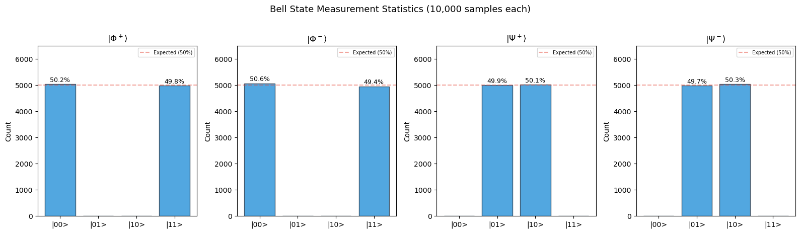
|Phi+> measurement results (10000 samples):
  |00>:  5009 (50.1%)
  |01>:     0 (0.0%)
  |10>:     0 (0.0%)
  |11>:  4991 (49.9%)
  Correlation: qubits agree 100.0% of the time
Observation
For \(|\Phi^+\rangle\) and \(|\Phi^-\rangle\), the two qubits are perfectly correlated (always agree). For \(|\Psi^+\rangle\) and \(|\Psi^-\rangle\), they are perfectly anti-correlated (always disagree). The difference between \(|\Phi^+\rangle\) and \(|\Phi^-\rangle\) (or \(|\Psi^+\rangle\) and \(|\Psi^-\rangle\)) is a relative phase that is invisible in the computational basis but detectable via interference.
Experiment 3: Deutsch-Jozsa Algorithm#
The Deutsch-Jozsa algorithm (1992) is the first demonstration of quantum speedup. Given a Boolean function \(f: \{0,1\}^n \to \{0,1\}\) promised to be either constant (same value on all inputs) or balanced (0 on exactly half of inputs), a classical computer needs \(2^{n-1}+1\) queries in the worst case to distinguish them. A quantum computer needs exactly one query.
We implement it for \(n = 2\) (4-input functions).
Show code cell source
import numpy as np
import math
import matplotlib.pyplot as plt


def deutsch_jozsa_oracle(f_values, n):
    """Build the oracle unitary for f: {0,1}^n -> {0,1}.

    The oracle acts on n+1 qubits: |x>|y> -> |x>|y XOR f(x)>.
    """
    N = 2 ** (n + 1)
    U = np.zeros((N, N), dtype=complex)
    for x in range(2 ** n):
        for y in range(2):
            input_idx = x * 2 + y
            output_y = y ^ f_values[x]
            output_idx = x * 2 + output_y
            U[output_idx, input_idx] = 1.0
    return U


def run_deutsch_jozsa(f_values, n):
    """Run the Deutsch-Jozsa algorithm.

    Returns
    -------
    result : str
        'constant' or 'balanced'
    probs : ndarray
        Measurement probabilities on input register.
    """
    dim = 2 ** (n + 1)
    H1 = np.array([[1, 1], [1, -1]], dtype=complex) / np.sqrt(2)
    I2 = np.eye(2, dtype=complex)

    # Step 1: Initialize |0>^n |1>
    state = np.zeros(dim, dtype=complex)
    state[1] = 1.0  # |00...0> |1>

    # Step 2: Apply H to all qubits
    H_all = np.eye(1, dtype=complex)
    for _ in range(n + 1):
        H_all = np.kron(H_all, H1)
    state = H_all @ state

    # Step 3: Apply oracle
    Uf = deutsch_jozsa_oracle(f_values, n)
    state = Uf @ state

    # Step 4: Apply H to input register only
    H_input = np.eye(1, dtype=complex)
    for _ in range(n):
        H_input = np.kron(H_input, H1)
    H_full = np.kron(H_input, I2)
    state = H_full @ state

    # Step 5: Measure input register
    probs_input = np.zeros(2 ** n)
    for x in range(2 ** n):
        for y in range(2):
            idx = x * 2 + y
            probs_input[x] += np.abs(state[idx]) ** 2

    result = 'constant' if probs_input[0] > 0.99 else 'balanced'
    return result, probs_input


# --- Test on all 2-bit oracles ---
n = 2
test_functions = {
    'f1 = 0 (constant)':     [0, 0, 0, 0],
    'f2 = 1 (constant)':     [1, 1, 1, 1],
    'f3 (balanced: 0011)':   [0, 0, 1, 1],
    'f4 (balanced: 0101)':   [0, 1, 0, 1],
    'f5 (balanced: 0110)':   [0, 1, 1, 0],
    'f6 (balanced: 1001)':   [1, 0, 0, 1],
}

fig, axes = plt.subplots(2, 3, figsize=(14, 8))

for ax, (fname, f_vals) in zip(axes.flat, test_functions.items()):
    result, probs = run_deutsch_jozsa(f_vals, n)

    basis_labels = [format(i, f'0{n}b') for i in range(2**n)]
    color = '#2ecc71' if result == 'constant' else '#e74c3c'
    ax.bar(basis_labels, probs, color=color, alpha=0.8,
           edgecolor='#2c3e50')
    ax.set_ylabel('Probability')
    ax.set_title(f'{fname}\nResult: {result}', fontsize=10)
    ax.set_ylim(0, 1.15)
    ax.set_xlabel('Measurement outcome')

    for i, p in enumerate(probs):
        if p > 0.01:
            ax.text(i, p + 0.03, f'{float(p):.2f}', ha='center', fontsize=9)

    print(f'{fname}: DJ says "{result}", P(|00>)={float(probs[0]):.4f}')

fig.suptitle('Deutsch-Jozsa Algorithm (n=2): One Query Distinguishes '
             'Constant from Balanced', fontsize=12, y=1.02)
plt.tight_layout()
plt.savefig('figures/ch37_fig3.png', dpi=150, bbox_inches='tight')
plt.show()
f1 = 0 (constant): DJ says "constant", P(|00>)=1.0000
f2 = 1 (constant): DJ says "constant", P(|00>)=1.0000
f3 (balanced: 0011): DJ says "balanced", P(|00>)=0.0000
f4 (balanced: 0101): DJ says "balanced", P(|00>)=0.0000
f5 (balanced: 0110): DJ says "balanced", P(|00>)=0.0000
f6 (balanced: 1001): DJ says "balanced", P(|00>)=0.0000
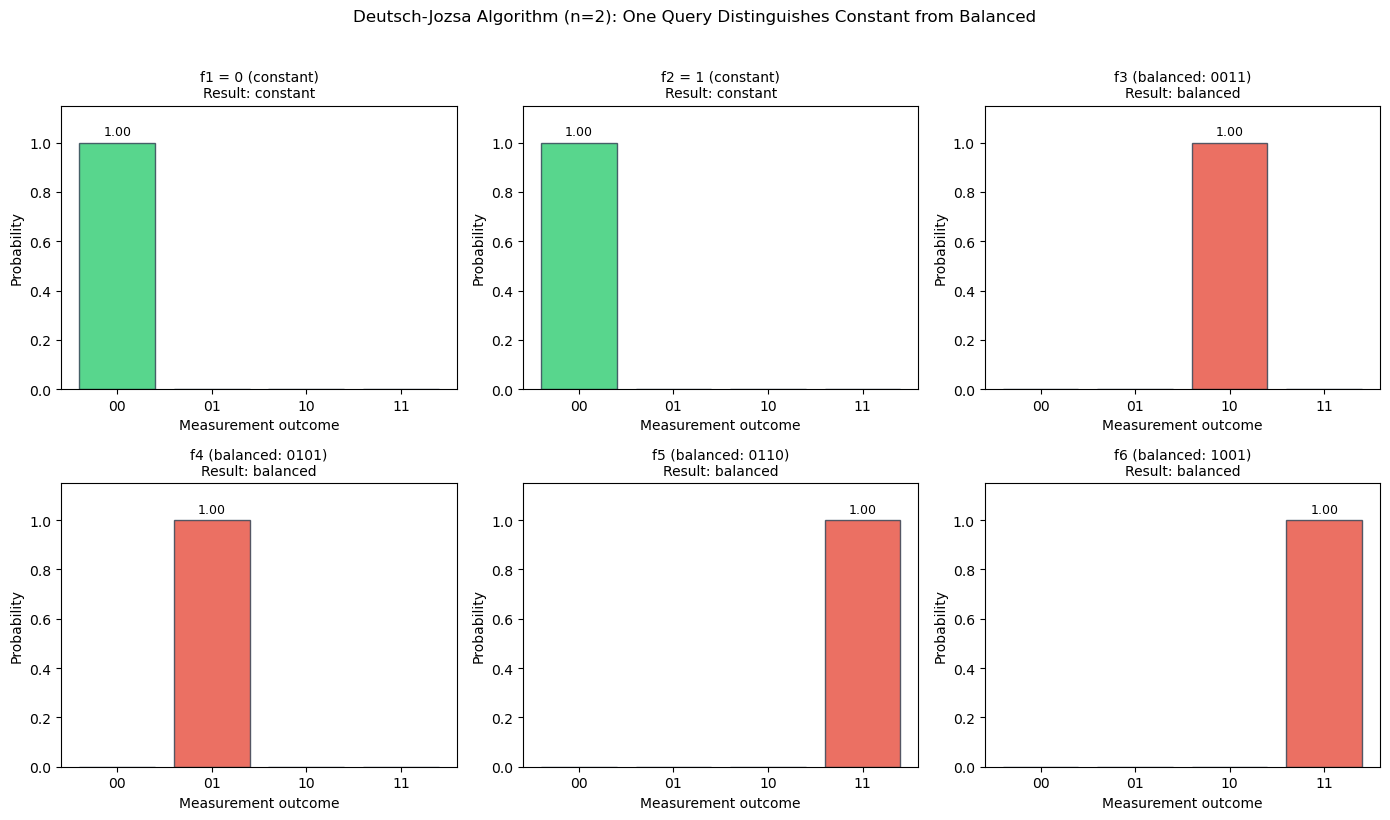
How It Works
The Deutsch-Jozsa circuit uses quantum interference to distinguish constant from balanced functions:
Prepare input qubits in \(|+\rangle^{\otimes n}\) and ancilla in \(|-\rangle\).
The oracle applies a phase \((-1)^{f(x)}\) to each basis state \(|x\rangle\) (phase kickback).
A final Hadamard transform causes constructive interference at \(|0\rangle^{\otimes n}\) if \(f\) is constant, and destructive interference if \(f\) is balanced.
This is the same interference principle that powers Shor’s algorithm.
Experiment 4: Quantum Teleportation Protocol#
Quantum teleportation transfers an arbitrary qubit state \(|\psi\rangle\) from Alice to Bob using one shared Bell pair and two classical bits. We simulate the full protocol step-by-step.
Show code cell source
import numpy as np
import math
import matplotlib.pyplot as plt


def fmt_amplitude(z):
    """Format a complex amplitude for display, preserving phase info."""
    if abs(z.imag) < 1e-10:
        return f'{z.real:+.3f}'
    elif abs(z.real) < 1e-10:
        return f'{z.imag:+.3f}i'
    else:
        return f'{z.real:.3f}{z.imag:+.3f}i'


def teleportation_protocol(alpha, beta, verbose=True):
    """Simulate quantum teleportation of state alpha|0> + beta|1>.

    Qubits: 0 = Alice's data, 1 = Alice's Bell, 2 = Bob's Bell.

    Returns
    -------
    bob_state : ndarray of shape (2,)
        Bob's final qubit state (should equal [alpha, beta]).
    alice_bits : tuple of (int, int)
        Alice's measurement outcomes.
    steps : list of (str, ndarray)
        State vector at each step.
    """
    H = np.array([[1, 1], [1, -1]], dtype=complex) / np.sqrt(2)
    I2 = np.eye(2, dtype=complex)
    CNOT = np.array([[1,0,0,0],[0,1,0,0],[0,0,0,1],[0,0,1,0]], dtype=complex)
    X = np.array([[0, 1], [1, 0]], dtype=complex)
    Z = np.array([[1, 0], [0, -1]], dtype=complex)

    steps = []

    # Step 0: Full initial state = |psi> x |0> x |0>
    psi = np.array([alpha, beta], dtype=complex)
    psi /= np.linalg.norm(psi)
    state = np.kron(np.kron(psi, [1, 0]), [1, 0])  # 8-dim
    steps.append(('Initial: |psi>|00>', state.copy()))
    if verbose:
        print(f'Step 0 (initial): |psi> = {fmt_amplitude(alpha)}|0> + {fmt_amplitude(beta)}|1>')

    # Step 1: Create Bell pair on qubits 1,2
    H_q1 = np.kron(np.kron(I2, H), I2)
    state = H_q1 @ state
    CNOT_12 = np.kron(I2, CNOT)
    state = CNOT_12 @ state
    steps.append(('Bell pair created', state.copy()))
    if verbose:
        print(f'Step 1 (Bell pair): shared entanglement between Alice and Bob')

    # Step 2: Alice applies CNOT q0->q1
    CNOT_01 = np.kron(CNOT, I2)
    state = CNOT_01 @ state
    steps.append(('CNOT q0->q1', state.copy()))

    # Step 3: Alice applies H to q0
    H_q0 = np.kron(np.kron(H, I2), I2)
    state = H_q0 @ state
    steps.append(('H on q0', state.copy()))
    if verbose:
        print(f'Step 2-3: Alice applies CNOT and H')

    # Step 4: Alice measures qubits 0 and 1
    probs_alice = np.zeros(4)
    bob_states = {}
    for m0 in range(2):
        for m1 in range(2):
            bob_state = np.zeros(2, dtype=complex)
            for b in range(2):
                idx = m0 * 4 + m1 * 2 + b
                bob_state[b] = state[idx]
            prob = np.linalg.norm(bob_state) ** 2
            probs_alice[m0 * 2 + m1] = prob
            if prob > 1e-10:
                bob_states[(m0, m1)] = bob_state / np.linalg.norm(bob_state)

    if verbose:
        print(f'Step 4: Alice measures:')
        for (m0, m1), bstate in bob_states.items():
            prob = probs_alice[m0 * 2 + m1]
            print(f'  ({m0},{m1}) prob={prob:.3f}: '
                  f'Bob has {fmt_amplitude(bstate[0])}|0> + {fmt_amplitude(bstate[1])}|1>')

    # Simulate one measurement
    flat_probs = probs_alice / probs_alice.sum()
    outcome = np.random.choice(4, p=flat_probs)
    m0, m1 = outcome // 2, outcome % 2
    bob_raw = bob_states[(m0, m1)]

    # Step 5: Bob applies corrections
    bob_corrected = bob_raw.copy()
    if m1 == 1:
        bob_corrected = X @ bob_corrected
    if m0 == 1:
        bob_corrected = Z @ bob_corrected

    # Fix global phase
    if np.abs(bob_corrected[0]) > 1e-10:
        phase = np.angle(psi[0]) - np.angle(bob_corrected[0])
        bob_corrected *= np.exp(1j * phase)

    if verbose:
        print(f'Step 5: Alice sends ({m0},{m1}), Bob corrects:')
        print(f'  Bob final: {fmt_amplitude(bob_corrected[0])}|0> + {fmt_amplitude(bob_corrected[1])}|1>')
        print(f'  Original:  {fmt_amplitude(psi[0])}|0> + {fmt_amplitude(psi[1])}|1>')
        fidelity = np.abs(np.dot(psi.conj(), bob_corrected)) ** 2
        print(f'  Fidelity: {fidelity:.6f}')

    return bob_corrected, (m0, m1), steps


# --- Test with several input states ---
test_states = [
    (1.0, 0.0, '|0>'),
    (0.0, 1.0, '|1>'),
    (1/np.sqrt(2), 1/np.sqrt(2), '|+>'),
    (np.cos(np.pi/8), np.sin(np.pi/8)*np.exp(1j*np.pi/3), 'general'),
]

np.random.seed(42)
fig, axes = plt.subplots(1, 4, figsize=(16, 4))

for ax, (alpha, beta, name) in zip(axes, test_states):
    print(f'\n--- Teleporting {name} ---')
    bob_state, alice_bits, steps = teleportation_protocol(alpha, beta)

    # Show state evolution (amplitudes)
    step_names = [s[0] for s in steps]
    norms = [np.abs(s[1]) for s in steps]
    n_steps = len(steps)
    n_amps = len(steps[0][1])
    basis = [format(i, '03b') for i in range(n_amps)]

    # Heatmap of amplitude magnitudes
    amp_matrix = np.array(norms)
    im = ax.imshow(amp_matrix.T, aspect='auto', cmap='YlOrRd',
                   vmin=0, vmax=1)
    ax.set_xticks(range(n_steps))
    ax.set_xticklabels([f'S{i}' for i in range(n_steps)],
                       fontsize=7, rotation=45)
    ax.set_yticks(range(n_amps))
    ax.set_yticklabels([f'|{b}>' for b in basis], fontsize=7)
    ax.set_title(f'Teleport {name}\nAlice: ({alice_bits[0]},{alice_bits[1]})',
                 fontsize=10)

fig.suptitle('Quantum Teleportation: Amplitude Evolution',
             fontsize=13, y=1.03)
plt.tight_layout()
plt.savefig('fig_ch37_teleportation.png', dpi=150, bbox_inches='tight')
plt.show()
--- Teleporting |0> ---
Step 0 (initial): |psi> = +1.000|0> + +0.000|1>
Step 1 (Bell pair): shared entanglement between Alice and Bob
Step 2-3: Alice applies CNOT and H
Step 4: Alice measures:
  (0,0) prob=0.250: Bob has +1.000|0> + +0.000|1>
  (0,1) prob=0.250: Bob has +0.000|0> + +1.000|1>
  (1,0) prob=0.250: Bob has +1.000|0> + +0.000|1>
  (1,1) prob=0.250: Bob has +0.000|0> + +1.000|1>
Step 5: Alice sends (0,1), Bob corrects:
  Bob final: +1.000|0> + +0.000|1>
  Original:  +1.000|0> + +0.000|1>
  Fidelity: 1.000000

--- Teleporting |1> ---
Step 0 (initial): |psi> = +0.000|0> + +1.000|1>
Step 1 (Bell pair): shared entanglement between Alice and Bob
Step 2-3: Alice applies CNOT and H
Step 4: Alice measures:
  (0,0) prob=0.250: Bob has +0.000|0> + +1.000|1>
  (0,1) prob=0.250: Bob has +1.000|0> + +0.000|1>
  (1,0) prob=0.250: Bob has +0.000|0> + -1.000|1>
  (1,1) prob=0.250: Bob has -1.000|0> + +0.000|1>
Step 5: Alice sends (1,1), Bob corrects:
  Bob final: +0.000|0> + +1.000|1>
  Original:  +0.000|0> + +1.000|1>
  Fidelity: 1.000000

--- Teleporting |+> ---
Step 0 (initial): |psi> = +0.707|0> + +0.707|1>
Step 1 (Bell pair): shared entanglement between Alice and Bob
Step 2-3: Alice applies CNOT and H
Step 4: Alice measures:
  (0,0) prob=0.250: Bob has +0.707|0> + +0.707|1>
  (0,1) prob=0.250: Bob has +0.707|0> + +0.707|1>
  (1,0) prob=0.250: Bob has +0.707|0> + -0.707|1>
  (1,1) prob=0.250: Bob has -0.707|0> + +0.707|1>
Step 5: Alice sends (1,0), Bob corrects:
  Bob final: +0.707|0> + +0.707|1>
  Original:  +0.707|0> + +0.707|1>
  Fidelity: 1.000000

--- Teleporting general ---
Step 0 (initial): |psi> = +0.924|0> + 0.191+0.331i|1>
Step 1 (Bell pair): shared entanglement between Alice and Bob
Step 2-3: Alice applies CNOT and H
Step 4: Alice measures:
  (0,0) prob=0.250: Bob has +0.924|0> + 0.191+0.331i|1>
  (0,1) prob=0.250: Bob has 0.191+0.331i|0> + +0.924|1>
  (1,0) prob=0.250: Bob has +0.924|0> + -0.191-0.331i|1>
  (1,1) prob=0.250: Bob has -0.191-0.331i|0> + +0.924|1>
Step 5: Alice sends (1,0), Bob corrects:
  Bob final: +0.924|0> + 0.191+0.331i|1>
  Original:  +0.924|0> + 0.191+0.331i|1>
  Fidelity: 1.000000
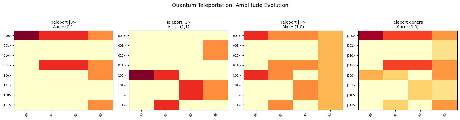
Teleportation Does Not Violate No-Cloning
Teleportation moves a quantum state; it does not copy it. Alice’s original qubit is destroyed by her measurement (collapsed to \(|m_0\rangle\)). The state reappears at Bob’s location only after he applies the correction gates, which require Alice’s classical measurement bits. Since these bits travel at most at the speed of light, teleportation cannot transmit information faster than light.
Experiment 5: Interference — Hadamard Sandwich#
The Mach-Zehnder interferometer is the quantum-optical analogue of the \(H\)–phase–\(H\) circuit. Applying \(H\), then a phase gate \(R_z(\phi)\), then \(H\) again creates constructive or destructive interference depending on \(\phi\). This is the fundamental mechanism behind every quantum algorithm.
Show code cell source
import numpy as np
import math
import matplotlib.pyplot as plt


H = np.array([[1, 1], [1, -1]], dtype=complex) / np.sqrt(2)

phi_values = np.linspace(0, 2 * np.pi, 500)
prob_0_list = []
prob_1_list = []

for phi in phi_values:
    Rz = np.array([[1, 0], [0, np.exp(1j * phi)]], dtype=complex)
    state = np.array([1, 0], dtype=complex)
    state = H @ state
    state = Rz @ state
    state = H @ state
    prob_0_list.append(np.abs(state[0])**2)
    prob_1_list.append(np.abs(state[1])**2)

fig, (ax1, ax2) = plt.subplots(1, 2, figsize=(14, 5))

# Left: Interference pattern
ax1.plot(phi_values / np.pi, prob_0_list, '-', color='#3498db',
         linewidth=2, label=r'$P(|0\rangle)$')
ax1.plot(phi_values / np.pi, prob_1_list, '--', color='#e74c3c',
         linewidth=2, label=r'$P(|1\rangle)$')
ax1.set_xlabel(r'Phase $\phi / \pi$', fontsize=11)
ax1.set_ylabel('Probability', fontsize=11)
ax1.set_title('Mach-Zehnder Interferometer\n'
              r'$|0\rangle \to H \to R_z(\phi) \to H \to$ measure',
              fontsize=11)
ax1.legend(fontsize=10)
ax1.grid(True, alpha=0.3)
ax1.set_xlim(0, 2)
ax1.set_ylim(-0.05, 1.05)

for phi_mark, label_mark in [(0, 'constructive'),
                              (1, 'destructive')]:
    ax1.axvline(x=phi_mark, color='gray', linestyle=':', alpha=0.5)
    ax1.annotate(label_mark, xy=(phi_mark, 0.5),
                 xytext=(phi_mark + 0.15, 0.7 if phi_mark == 0 else 0.3),
                 fontsize=9, arrowprops=dict(arrowstyle='->', color='gray'))

# Right: Specific gate sandwiches
gate_names = ['Z', 'S', 'T', 'I']
gate_matrices = [
    np.array([[1,0],[0,-1]], dtype=complex),
    np.array([[1,0],[0,1j]], dtype=complex),
    np.array([[1,0],[0,np.exp(1j*np.pi/4)]], dtype=complex),
    np.eye(2, dtype=complex)
]

bar_data = []
for gname, gmat in zip(gate_names, gate_matrices):
    state = np.array([1, 0], dtype=complex)
    state = H @ state
    state = gmat @ state
    state = H @ state
    p0 = np.abs(state[0])**2
    bar_data.append(p0)

colors2 = ['#e74c3c', '#e67e22', '#f1c40f', '#2ecc71']
ax2.bar(gate_names, bar_data, color=colors2, alpha=0.85,
        edgecolor='#2c3e50')
ax2.set_ylabel(r'$P(|0\rangle)$', fontsize=11)
ax2.set_xlabel('Middle gate', fontsize=11)
ax2.set_title(r'$H \to G \to H$ interference results', fontsize=11)
ax2.set_ylim(0, 1.15)
for i, val in enumerate(bar_data):
    ax2.text(i, val + 0.03, f'{float(val):.3f}', ha='center', fontsize=10)

plt.tight_layout()
plt.savefig('figures/ch37_fig5.png', dpi=150, bbox_inches='tight')
plt.show()

print('Hadamard sandwich results (H-G-H applied to |0>):')
for gname, p0 in zip(gate_names, bar_data):
    print(f'  G = {gname}: P(|0>) = {float(p0):.4f}, P(|1>) = {float(1-p0):.4f}')
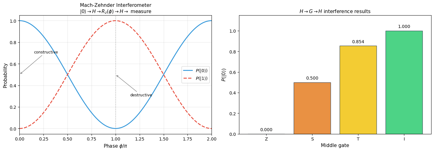
Hadamard sandwich results (H-G-H applied to |0>):
  G = Z: P(|0>) = 0.0000, P(|1>) = 1.0000
  G = S: P(|0>) = 0.5000, P(|1>) = 0.5000
  G = T: P(|0>) = 0.8536, P(|1>) = 0.1464
  G = I: P(|0>) = 1.0000, P(|1>) = 0.0000
The Key Insight for Quantum Algorithms
Quantum algorithms work by orchestrating constructive interference on correct answers and destructive interference on wrong answers. The Hadamard sandwich \(H\)-phase-\(H\) is the simplest example:
\(\phi = 0\) (identity): \(H \cdot I \cdot H = I\), so \(|0\rangle \to |0\rangle\) — constructive.
\(\phi = \pi\) (\(Z\) gate): \(H \cdot Z \cdot H = X\), so \(|0\rangle \to |1\rangle\) — destructive.
Shor’s algorithm uses the QFT to create interference patterns that reveal the period of modular exponentiation. Grover’s algorithm uses the “inversion about the mean” operator to amplify the amplitude of the target.
Experiment 6: No-Cloning Demonstration#
We demonstrate the no-cloning theorem computationally: we show that no unitary can simultaneously clone \(|0\rangle\), \(|1\rangle\), and \(|+\rangle\). A CNOT gate acts as a cloner for \(|0\rangle\) and \(|1\rangle\) but fails for superposition states.
Show code cell source
import numpy as np
import math
import matplotlib.pyplot as plt


CNOT = np.array([[1,0,0,0],[0,1,0,0],[0,0,0,1],[0,0,1,0]], dtype=complex)

test_states = {
    '|0>': np.array([1, 0], dtype=complex),
    '|1>': np.array([0, 1], dtype=complex),
    '|+>': np.array([1, 1], dtype=complex) / np.sqrt(2),
    '|->': np.array([1, -1], dtype=complex) / np.sqrt(2),
    '|i>': np.array([1, 1j], dtype=complex) / np.sqrt(2),
}

print('Attempting to clone states using CNOT as a cloner:')
print(f'{"State":>6} | {"Is clone correct?":>20} | {"Fidelity":>10}')
print('=' * 45)

results = {}
for name, psi in test_states.items():
    input_state = np.kron(psi, [1, 0])
    output_state = CNOT @ input_state
    desired = np.kron(psi, psi)
    overlap = np.abs(np.dot(desired.conj(), output_state)) ** 2
    is_clone = overlap > 0.999
    results[name] = (is_clone, overlap, output_state, desired)
    print(f'{name:>6} | {"YES" if is_clone else "NO":>20} | {float(overlap):>10.4f}')

# Visualization
fig, (ax1, ax2) = plt.subplots(1, 2, figsize=(14, 5.5))

# Sweep over Bloch sphere
n_theta = 100
n_phi = 100
thetas = np.linspace(0, np.pi, n_theta)
phis = np.linspace(0, 2 * np.pi, n_phi)
fidelity_map = np.zeros((n_theta, n_phi))

for i, theta in enumerate(thetas):
    for j, phi in enumerate(phis):
        alpha = np.cos(theta / 2)
        beta = np.exp(1j * phi) * np.sin(theta / 2)
        psi = np.array([alpha, beta], dtype=complex)
        input_state = np.kron(psi, [1, 0])
        output = CNOT @ input_state
        desired = np.kron(psi, psi)
        fidelity_map[i, j] = np.abs(np.dot(desired.conj(), output)) ** 2

im = ax1.imshow(fidelity_map, extent=[0, 2, 0, 1],
                aspect='auto', cmap='RdYlGn', vmin=0, vmax=1,
                origin='lower')
ax1.set_xlabel(r'$\phi / \pi$', fontsize=11)
ax1.set_ylabel(r'$\theta / \pi$', fontsize=11)
ax1.set_title('CNOT Cloning Fidelity Across Bloch Sphere', fontsize=11)
plt.colorbar(im, ax=ax1, label='Fidelity')

special = [
    (0, 0, '|0>'), (1, 0, '|1>'),
    (0.5, 0, '|+>'), (0.5, 1, '|->')
]
for theta_pi, phi_pi, lbl in special:
    col = '#2ecc71' if theta_pi in [0, 1] else '#e74c3c'
    ax1.plot(phi_pi, theta_pi, 'o', color=col, markersize=8)
    ax1.annotate(lbl, (phi_pi + 0.05, theta_pi + 0.03), fontsize=9, color=col)

# Bar chart
names = list(results.keys())
fids = [results[n][1] for n in names]
colors = ['#2ecc71' if f > 0.99 else '#e74c3c' for f in fids]
ax2.bar(names, fids, color=colors, alpha=0.85, edgecolor='#2c3e50')
ax2.set_ylabel('Cloning Fidelity', fontsize=11)
ax2.set_title('CNOT Cloning: Only Works for\nComputational Basis States', fontsize=11)
ax2.set_ylim(0, 1.15)
ax2.axhline(y=1.0, color='gray', linestyle='--', alpha=0.5)
for i, f in enumerate(fids):
    ax2.text(i, f + 0.03, f'{float(f):.3f}', ha='center', fontsize=10)

plt.tight_layout()
plt.savefig('figures/ch37_fig6.png', dpi=150, bbox_inches='tight')
plt.show()
Attempting to clone states using CNOT as a cloner:
 State |    Is clone correct? |   Fidelity
=============================================
   |0> |                  YES |     1.0000
   |1> |                  YES |     1.0000
   |+> |                   NO |     0.5000
   |-> |                   NO |     0.0000
   |i> |                   NO |     0.2500
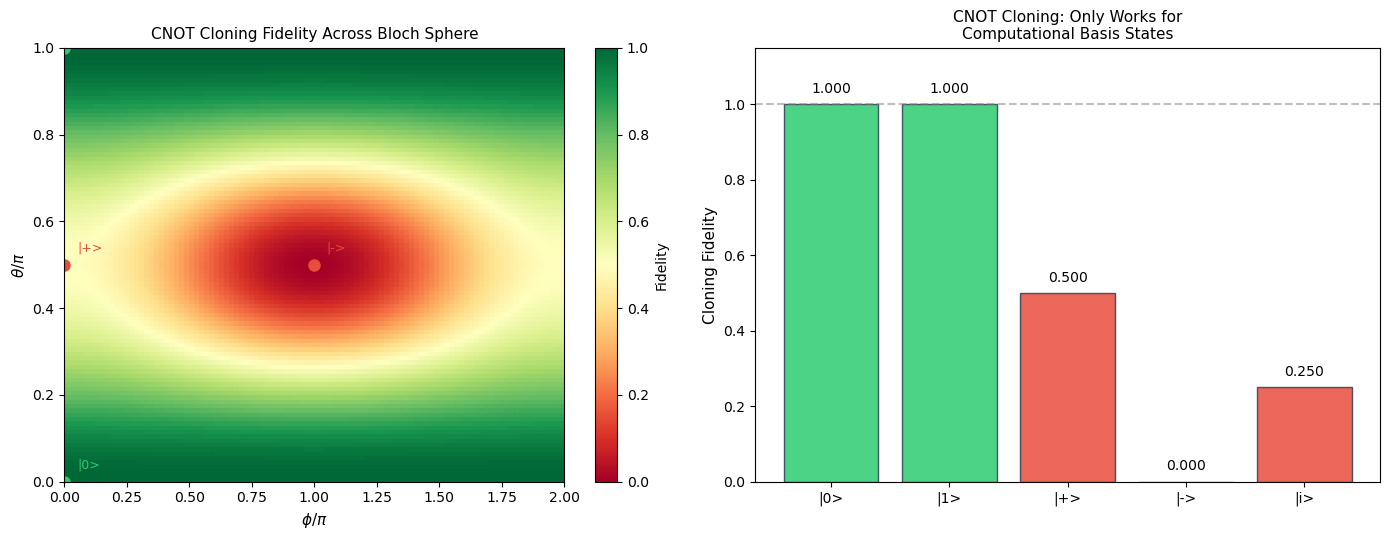
No-Cloning in Action
CNOT perfectly clones \(|0\rangle\) and \(|1\rangle\):
\(\text{CNOT}|0\rangle|0\rangle = |00\rangle = |0\rangle|0\rangle\) (correct clone)
\(\text{CNOT}|1\rangle|0\rangle = |11\rangle = |1\rangle|1\rangle\) (correct clone)
But for \(|+\rangle = \frac{1}{\sqrt{2}}(|0\rangle + |1\rangle)\):
\(\text{CNOT}|+\rangle|0\rangle = \frac{1}{\sqrt{2}}(|00\rangle + |11\rangle) = |\Phi^+\rangle\)
Desired: \(|+\rangle|+\rangle = \frac{1}{2}(|00\rangle + |01\rangle + |10\rangle + |11\rangle)\)
Instead of a clone, CNOT produces an entangled state! This is exactly the no-cloning theorem at work: linearity of quantum mechanics prevents cloning superpositions.
37.5 Exercises#
Exercise 37.1 (Warm-up: Gate Arithmetic)
Verify by matrix multiplication that \(HXH = Z\), \(HZH = X\), and \(H^2 = I\). What does this tell you about the relationship between bit-flip and phase-flip errors in the Hadamard basis?
Hint
Compute the products directly: \(HXH = \frac{1}{2}\begin{pmatrix}1&1\\1&-1\end{pmatrix}\begin{pmatrix}0&1\\1&0\end{pmatrix}\begin{pmatrix}1&1\\1&-1\end{pmatrix} = \begin{pmatrix}1&0\\0&-1\end{pmatrix} = Z.\) This means a bit-flip in the computational basis becomes a phase-flip in the Hadamard basis, and vice versa. Error correction must handle both types.
Exercise 37.2 (Multi-Qubit States)
Write out the full 8-component state vector for \(|\psi\rangle = |+\rangle \otimes |1\rangle \otimes |0\rangle\). What is the probability of measuring \(|110\rangle\)?
Hint
\(|+\rangle = \frac{1}{\sqrt{2}}(|0\rangle + |1\rangle)\), so \(|\psi\rangle = \frac{1}{\sqrt{2}}(|010\rangle + |110\rangle)\). The state vector is \(\frac{1}{\sqrt{2}}(0, 0, 1, 0, 0, 0, 1, 0)^T\). The probability of \(|110\rangle\) is \(|1/\sqrt{2}|^2 = 1/2\).
Exercise 37.3 (Entanglement Detection)
Given the state \(|\psi\rangle = \frac{1}{2}(|00\rangle + |01\rangle + |10\rangle + |11\rangle)\), is this state entangled? Prove your answer by attempting to factor it as a tensor product.
Hint
Write \(|\psi\rangle = \frac{1}{2}(|0\rangle + |1\rangle)(|0\rangle + |1\rangle) = |+\rangle|+\rangle\). This is a product state, so it is not entangled. Compare with \(|\Phi^+\rangle = \frac{1}{\sqrt{2}}(|00\rangle + |11\rangle)\), which cannot be factored (try: \(\alpha\gamma = 1/\sqrt{2}\), \(\alpha\delta = 0\), \(\beta\gamma = 0\), \(\beta\delta = 1/\sqrt{2}\) — no solution).
Exercise 37.4 (Circuit Design)
Design a quantum circuit that creates the GHZ state
\(|\text{GHZ}\rangle = \frac{1}{\sqrt{2}}(|000\rangle + |111\rangle)\)
on 3 qubits. Implement it using the QuantumCircuit class and verify
by examining the output probabilities.
Hint
Apply \(H\) to qubit 0, then CNOT from qubit 0 to qubit 1, then CNOT from qubit 0 to qubit 2 (or equivalently, CNOT from qubit 1 to qubit 2). The circuit generalizes the Bell state construction to 3 qubits.
Exercise 37.5 (Challenge: Superdense Coding)
Implement the superdense coding protocol: Alice sends 2 classical bits to Bob by transmitting only 1 qubit (using a pre-shared Bell pair). Show that Bob can distinguish all four of Alice’s messages.
Hint
Alice and Bob share \(|\Phi^+\rangle\). To send bits \((b_1, b_2)\), Alice applies: nothing for 00, \(X\) for 01, \(Z\) for 10, \(XZ\) for 11, then sends her qubit to Bob. Bob applies CNOT then \(H\) and measures both qubits to recover \((b_1, b_2)\).
37.6 Summary#
Concept |
Key Point |
|---|---|
Qubit |
Unit vector in \(\mathbb{C}^2\): $\alpha |
Superposition |
A qubit can be in a weighted combination of $ |
Bloch sphere |
Geometric representation: \(\theta, \phi\) parameterize all pure qubit states |
Quantum gates |
Unitary matrices; \(\{H, T, \text{CNOT}\}\) is universal |
Measurement |
Born rule: outcome \(x\) with probability $ |
Tensor product |
\(n\)-qubit state lives in \(\mathbb{C}^{2^n}\) — exponential state space |
Entanglement |
Non-separable states; perfect correlations without classical communication |
No-cloning |
Cannot copy unknown quantum states; enables QKD |
Interference |
Constructive/destructive amplitude combination — the engine of quantum speedup |
Deutsch-Jozsa |
Oracle distinction in 1 query vs. \(2^{n-1}+1\) classically |
Teleportation |
Transfer qubit state using Bell pair + 2 classical bits |
Tip
The three pillars of quantum computing that enable cryptanalytic speedups are:
Superposition: process \(2^n\) values simultaneously.
Interference: amplify correct answers, suppress wrong ones.
Entanglement: create correlations impossible classically.
In Chapter 38, we will see how Shor combines these with the Quantum Fourier Transform to break RSA and Diffie-Hellman. In Chapter 39, Grover uses them to speed up brute-force search quadratically.
References#
Nielsen, M. A. and Chuang, I. L. (2010). Quantum Computation and Quantum Information. 10th Anniversary Edition, Cambridge University Press.
Preskill, J. (1998–2023). Lecture Notes on Quantum Computation. Caltech, available at http://theory.caltech.edu/~preskill/ph219/.
Mermin, N. D. (2007). Quantum Computer Science: An Introduction. Cambridge University Press.
Rieffel, E. G. and Polak, W. H. (2011). Quantum Computing: A Gentle Introduction. MIT Press.
Feynman, R. P. (1982). Simulating physics with computers. International Journal of Theoretical Physics, 21(6/7), 467–488.
Deutsch, D. (1985). Quantum theory, the Church-Turing principle and the universal quantum computer. Proceedings of the Royal Society A, 400, 97–117.
Deutsch, D. and Jozsa, R. (1992). Rapid solution of problems by quantum computation. Proceedings of the Royal Society A, 439, 553–558.
Bernstein, E. and Vazirani, U. (1993). Quantum complexity theory. Proceedings of the 25th ACM STOC, 11–20.
Simon, D. (1994). On the power of quantum computation. Proceedings of the 35th IEEE FOCS, 116–123.
Wootters, W. K. and Zurek, W. H. (1982). A single quantum cannot be cloned. Nature, 299, 802–803.
Bennett, C. H. et al. (1993). Teleporting an unknown quantum state via dual classical and Einstein-Podolsky-Rosen channels. Physical Review Letters, 70(13), 1895–1899.