
Chapter 24 — AES Security and the Wide Trail Strategy#
“The wide trail strategy is a design philosophy, not a proof technique.” — Joan Daemen and Vincent Rijmen, The Design of Rijndael, 2002
In this chapter we study how AES was specifically designed to resist linear and differential cryptanalysis. We formalize the wide trail strategy of Daemen and Rijmen, define the branch number of a linear transformation, count active S-boxes across multiple AES rounds, and quantify the security margins that make AES the dominant symmetric cipher of the 21st century.
24.1 Historical Context#
After DES fell to advances in both hardware (EFF Deep Crack, 1998) and cryptanalysis (Matsui’s linear attack, 1993; Biham–Shamir differential attack, 1991), NIST launched the Advanced Encryption Standard competition in 1997. Among the 15 submissions, Rijndael (by Joan Daemen and Vincent Rijmen of Belgium) was selected in October 2000 and standardized as FIPS 197 in 2001.
Crucially, Rijndael was not designed merely to be fast or elegant – it was engineered from the ground up to provide provable resistance to the two most powerful known attacks on block ciphers:
Attack |
Year |
DES Vulnerability |
AES Design Response |
|---|---|---|---|
Differential (Biham–Shamir) |
1991 |
\(2^{47}\) chosen plaintexts |
Max differential probability \(\leq 2^{-150}\) (full AES) |
Linear (Matsui) |
1993 |
\(2^{43}\) known plaintexts |
Max linear bias \(\leq 2^{-75}\) (full AES) |
The key innovation was the wide trail strategy: by carefully choosing the linear mixing layer (MixColumns), the designers guaranteed that any differential or linear trail must activate a minimum number of S-boxes, making the probability of any trail exponentially small.
Tip
The AES competition was the first major standardization effort where resistance to differential and linear cryptanalysis was an explicit, quantified design goal. This philosophy – design for provable resistance – has influenced every subsequent block cipher and permutation-based design.
24.2 Key Concepts#
24.2.1 The Branch Number#
The branch number is the central quantity in the wide trail strategy. It measures how effectively a linear transformation spreads differences (for differential attacks) or correlations (for linear attacks).
Definition 24.1 — Branch Number of a Linear Transformation
Let \(\theta: \mathrm{GF}(2^n)^c \to \mathrm{GF}(2^n)^c\) be a linear transformation. The branch number of \(\theta\) is:
where \(w(a)\) denotes the number of nonzero components (bytes, in AES) of \(a\).
The branch number tells us: if we feed a nonzero input into \(\theta\), the total number of nonzero bytes in the input plus the output is at least \(\mathcal{B}(\theta)\). A higher branch number means better diffusion.
Definition 24.2 — Differential and Linear Branch Numbers
For a linear transformation \(\theta\) over \(\mathrm{GF}(2^8)^4\) (as in AES MixColumns, which operates on 4-byte columns):
Differential branch number: \(\mathcal{B}_d(\theta) = \min_{a \neq 0} \{ w(a) + w(\theta(a)) \}\)
Linear branch number: \(\mathcal{B}_l(\theta) = \min_{a \neq 0} \{ w(a) + w(\theta^T(a)) \}\)
For AES MixColumns, both are equal to 5 — the maximum possible value for a \(4 \times 4\) matrix (since \(\mathcal{B} \leq c + 1 = 5\)).
Important
A branch number of 5 for MixColumns means it is a maximum distance separable (MDS) code. The MixColumns matrix \(\begin{pmatrix} 2&3&1&1 \\ 1&2&3&1 \\ 1&1&2&3 \\ 3&1&1&2 \end{pmatrix}\) over \(\mathrm{GF}(2^8)\) has this property because every square submatrix is invertible.
24.2.2 Active S-Boxes#
Definition 24.3 — Active S-Boxes
An S-box is active in a differential (or linear) trail if it receives a nonzero input difference (or has a nonzero input mask). The security of a cipher depends on the minimum number of active S-boxes across all possible trails spanning \(r\) rounds.
For AES:
4 rounds: minimum 25 active S-boxes
Any \(r\) rounds (\(r \geq 4\)): minimum \(\lceil 25 \cdot r/4 \rceil\) active S-boxes (approximately)
Theorem 24.1 — Wide Trail Strategy
Let \(p_{\max}\) be the maximum differential probability (or squared linear correlation) of the AES S-box. If the minimum number of active S-boxes over \(r\) rounds is \(n_r\), then the maximum probability of any \(r\)-round differential characteristic is bounded by:
For AES: \(p_{\max} = 2^{-6}\) (the S-box has differential uniformity 4, so \(p_{\max} = 4/256 = 2^{-6}\)). Over 4 rounds with 25 active S-boxes:
Since \(2^{-150} \ll 2^{-128}\), even a 4-round differential attack requires more data than exists in the key space. Full 10-round AES-128 is therefore far beyond the reach of classical differential cryptanalysis.
Proof sketch
The proof proceeds in two steps:
Branch number argument. The ShiftRows + MixColumns combination ensures that any trail through two consecutive rounds activates at least \(\mathcal{B}(\text{MixColumns}) = 5\) S-boxes per active column. Since ShiftRows distributes bytes from one column across all four columns, even a single active byte in one round forces activity in multiple columns in the next round.
Counting argument. Over 4 rounds, the minimum is achieved by a trail with 1 active byte entering round 1, which expands to at least 5 in round 2 (by branch number), which in turn expands to at least \(5 \times 5 = 25\). The detailed proof uses the structure of ShiftRows to show this bound is tight.
Each active S-box contributes at most \(p_{\max}\) to the trail probability (by independence), giving the bound. \(\square\)
24.2.3 Security Margins#
AES Security Margins
AES-128 uses a 128-bit key and 10 rounds. The best known attacks are:
Attack |
Rounds broken |
Complexity |
Reference |
|---|---|---|---|
Biclique (key recovery) |
10 (full) |
\(2^{126.1}\) |
Bogdanov et al. 2011 |
Differential |
8 |
\(2^{128}\) (impractical) |
|
Linear |
7 |
\(2^{128}\) (impractical) |
|
Square/Integral |
7 |
\(2^{128}\) (impractical) |
The biclique attack improves over brute force by a factor of only \(\sim 4\), which is negligible. No practical attack on full AES exists.
24.3 Implementation#
24.3.1 AES S-Box and GF(\(2^8\)) Arithmetic#
We begin by implementing the AES S-box and the Galois field arithmetic needed for MixColumns. All operations are in \(\mathrm{GF}(2^8)\) with the irreducible polynomial \(x^8 + x^4 + x^3 + x + 1\) (0x11B).
import numpy as np

# --- GF(2^8) arithmetic with irreducible polynomial x^8+x^4+x^3+x+1 ---

def gf_mul(a, b, mod=0x11B):
    """Multiply two elements in GF(2^8)."""
    result = 0
    a = int(a)
    b = int(b)
    for _ in range(8):
        if b & 1:
            result ^= a
        a <<= 1
        if a & 0x100:
            a ^= mod
        b >>= 1
    return result


def gf_inv(a, mod=0x11B):
    """Multiplicative inverse in GF(2^8) using extended Euclidean algorithm."""
    if a == 0:
        return 0
    # Use Fermat's little theorem: a^(-1) = a^(254) in GF(2^8)
    result = a
    for _ in range(6):  # square-and-multiply for a^254
        result = gf_mul(result, result, mod)
        result = gf_mul(result, a, mod)
    result = gf_mul(result, result, mod)
    return result


# Build the AES S-box
def build_aes_sbox():
    """Construct the AES S-box: inversion in GF(2^8) + affine transform."""
    sbox = np.zeros(256, dtype=np.uint8)
    # Affine transformation matrix (over GF(2))
    affine_matrix = np.array([
        [1, 0, 0, 0, 1, 1, 1, 1],
        [1, 1, 0, 0, 0, 1, 1, 1],
        [1, 1, 1, 0, 0, 0, 1, 1],
        [1, 1, 1, 1, 0, 0, 0, 1],
        [1, 1, 1, 1, 1, 0, 0, 0],
        [0, 1, 1, 1, 1, 1, 0, 0],
        [0, 0, 1, 1, 1, 1, 1, 0],
        [0, 0, 0, 1, 1, 1, 1, 1],
    ], dtype=np.uint8)
    affine_const = np.array([1, 1, 0, 0, 0, 1, 1, 0], dtype=np.uint8)  # 0x63

    for i in range(256):
        inv = gf_inv(i)
        # Convert to bit vector (LSB first)
        bits = np.array([(inv >> j) & 1 for j in range(8)], dtype=np.uint8)
        # Apply affine transformation
        out_bits = (affine_matrix @ bits + affine_const) % 2
        # Convert back to byte
        val = sum(int(out_bits[j]) << j for j in range(8))
        sbox[i] = val

    return sbox


AES_SBOX = build_aes_sbox()

# Verify against known values
assert AES_SBOX[0x00] == 0x63, f"S(0x00) should be 0x63, got {AES_SBOX[0x00]:#x}"
assert AES_SBOX[0x01] == 0x7C, f"S(0x01) should be 0x7C, got {AES_SBOX[0x01]:#x}"
assert AES_SBOX[0x53] == 0xED, f"S(0x53) should be 0xED, got {AES_SBOX[0x53]:#x}"
assert AES_SBOX[0xFF] == 0x16, f"S(0xFF) should be 0x16, got {AES_SBOX[0xFF]:#x}"

print("AES S-box constructed and verified.")
print(f"S(0x00) = 0x{AES_SBOX[0x00]:02X}")
print(f"S(0x01) = 0x{AES_SBOX[0x01]:02X}")
print(f"S(0xFF) = 0x{AES_SBOX[0xFF]:02X}")
print()

# Display S-box as 16x16 table
print("AES S-box (hex):")
print("     " + " ".join(f" {j:X}" for j in range(16)))
print("    " + "-" * 50)
for i in range(16):
    row = " ".join(f"{AES_SBOX[16*i + j]:02X}" for j in range(16))
    print(f" {i:X} | {row}")
AES S-box constructed and verified.
S(0x00) = 0x63
S(0x01) = 0x7C
S(0xFF) = 0x16

AES S-box (hex):
      0  1  2  3  4  5  6  7  8  9  A  B  C  D  E  F
    --------------------------------------------------
 0 | 63 7C 77 7B F2 6B 6F C5 30 01 67 2B FE D7 AB 76
 1 | CA 82 C9 7D FA 59 47 F0 AD D4 A2 AF 9C A4 72 C0
 2 | B7 FD 93 26 36 3F F7 CC 34 A5 E5 F1 71 D8 31 15
 3 | 04 C7 23 C3 18 96 05 9A 07 12 80 E2 EB 27 B2 75
 4 | 09 83 2C 1A 1B 6E 5A A0 52 3B D6 B3 29 E3 2F 84
 5 | 53 D1 00 ED 20 FC B1 5B 6A CB BE 39 4A 4C 58 CF
 6 | D0 EF AA FB 43 4D 33 85 45 F9 02 7F 50 3C 9F A8
 7 | 51 A3 40 8F 92 9D 38 F5 BC B6 DA 21 10 FF F3 D2
 8 | CD 0C 13 EC 5F 97 44 17 C4 A7 7E 3D 64 5D 19 73
 9 | 60 81 4F DC 22 2A 90 88 46 EE B8 14 DE 5E 0B DB
 A | E0 32 3A 0A 49 06 24 5C C2 D3 AC 62 91 95 E4 79
 B | E7 C8 37 6D 8D D5 4E A9 6C 56 F4 EA 65 7A AE 08
 C | BA 78 25 2E 1C A6 B4 C6 E8 DD 74 1F 4B BD 8B 8A
 D | 70 3E B5 66 48 03 F6 0E 61 35 57 B9 86 C1 1D 9E
 E | E1 F8 98 11 69 D9 8E 94 9B 1E 87 E9 CE 55 28 DF
 F | 8C A1 89 0D BF E6 42 68 41 99 2D 0F B0 54 BB 16
24.3.2 Computing the Branch Number of MixColumns#
We compute the branch number by exhaustive search over all nonzero 4-byte inputs, evaluating \(w(a) + w(\text{MixColumns}(a))\) where \(w\) counts nonzero bytes.
Verification scope
Weight-1 inputs are checked exhaustively; weight-2 inputs are verified by sampling. A complete proof requires checking all \(\binom{255 \times 4}{2}\) weight-2 inputs.
import numpy as np

# AES MixColumns matrix over GF(2^8)
MC_MATRIX = np.array([
    [2, 3, 1, 1],
    [1, 2, 3, 1],
    [1, 1, 2, 3],
    [3, 1, 1, 2]
], dtype=int)


def gf_mul(a, b, mod=0x11B):
    """Multiply two elements in GF(2^8)."""
    result = 0
    a, b = int(a), int(b)
    for _ in range(8):
        if b & 1:
            result ^= a
        a <<= 1
        if a & 0x100:
            a ^= mod
        b >>= 1
    return result


def mix_column(col, matrix=MC_MATRIX):
    """Apply MixColumns to a single 4-byte column."""
    out = np.zeros(4, dtype=int)
    for i in range(4):
        val = 0
        for j in range(4):
            val ^= gf_mul(matrix[i, j], col[j])
        out[i] = val
    return out


def byte_weight(vec):
    """Count number of nonzero bytes in a vector."""
    return int(np.sum(np.array(vec) != 0))


def compute_branch_number_exact(matrix):
    """
    Compute the differential branch number of a 4x4 matrix over GF(2^8)
    by exhaustive search over all nonzero 4-byte inputs.

    This requires checking 2^32 - 1 inputs, which is too many.
    Instead, we use the MDS property: check all inputs with weight 1
    and weight 2 to establish the lower bound.
    """
    min_branch = 9  # Upper bound: 4+4+1

    # Weight-1 inputs: one nonzero byte (255 values x 4 positions = 1020)
    for pos in range(4):
        for val in range(1, 256):
            inp = np.zeros(4, dtype=int)
            inp[pos] = val
            out = mix_column(inp, matrix)
            branch = byte_weight(inp) + byte_weight(out)
            min_branch = min(min_branch, branch)

    # Weight-2 inputs: two nonzero bytes (C(4,2) * 255^2 = 6 * 65025)
    from itertools import combinations
    for positions in combinations(range(4), 2):
        for v1 in range(1, 256):
            for v2 in range(1, 256):
                inp = np.zeros(4, dtype=int)
                inp[positions[0]] = v1
                inp[positions[1]] = v2
                out = mix_column(inp, matrix)
                branch = byte_weight(inp) + byte_weight(out)
                min_branch = min(min_branch, branch)
                if min_branch <= 4:
                    # If we find branch <= 4, it is not MDS
                    # but we continue to find the true minimum
                    pass

    return min_branch


# A faster approach: since for weight-1, output weight >= 4 gives branch >= 5,
# and for weight >= 3, branch >= 3 + 1 = 4 (trivially), the critical case is
# weight-1 and weight-2 inputs.

# For weight-1 inputs:
print("Checking weight-1 inputs (1020 cases)...")
min_branch_w1 = 9
for pos in range(4):
    for val in range(1, 256):
        inp = np.zeros(4, dtype=int)
        inp[pos] = val
        out = mix_column(inp)
        branch = byte_weight(inp) + byte_weight(out)
        min_branch_w1 = min(min_branch_w1, branch)

print(f"  Minimum branch number (weight-1 inputs): {min_branch_w1}")
print(f"  Output always has weight >= {min_branch_w1 - 1} for weight-1 input")
print()

# For a sample of weight-2 inputs:
print("Checking weight-2 inputs (sample of 50000 cases)...")
rng = np.random.default_rng(42)
min_branch_w2 = 9
n_samples = 50000
for _ in range(n_samples):
    positions = rng.choice(4, size=2, replace=False)
    inp = np.zeros(4, dtype=int)
    inp[positions[0]] = rng.integers(1, 256)
    inp[positions[1]] = rng.integers(1, 256)
    out = mix_column(inp)
    branch = byte_weight(inp) + byte_weight(out)
    min_branch_w2 = min(min_branch_w2, branch)

print(f"  Minimum branch number (weight-2 sample): {min_branch_w2}")
print()

# Weight-3 and weight-4 inputs trivially have branch >= 3+1=4, 4+1=5
# (since MixColumns is invertible, output is always nonzero for nonzero input)
print("Weight-3 inputs: branch >= 3 + w(out) >= 3 + 1 = 4 (but MDS gives 5)")
print("Weight-4 inputs: branch >= 4 + w(out) >= 4 + 1 = 5")
print()
print(f"==> Branch number of AES MixColumns = {min(min_branch_w1, min_branch_w2)}")
print("    This equals c+1 = 5, confirming MDS property.")
Checking weight-1 inputs (1020 cases)...
  Minimum branch number (weight-1 inputs): 5
  Output always has weight >= 4 for weight-1 input

Checking weight-2 inputs (sample of 50000 cases)...
  Minimum branch number (weight-2 sample): 5

Weight-3 inputs: branch >= 3 + w(out) >= 3 + 1 = 4 (but MDS gives 5)
Weight-4 inputs: branch >= 4 + w(out) >= 4 + 1 = 5

==> Branch number of AES MixColumns = 5
    This equals c+1 = 5, confirming MDS property.
Why branch number 5 is optimal
For a \(c \times c\) matrix over \(\mathrm{GF}(2^n)\), the maximum possible branch number is \(c + 1\). This is because: if the input has weight \(w\), then \(w(a) + w(\theta(a)) \leq w + c\). Equality is achieved when every nonzero input byte produces a fully nonzero output – i.e., the matrix is MDS. AES achieves this maximum: \(\mathcal{B} = 4 + 1 = 5\).
24.3.3 Counting Minimum Active S-Boxes#
We now compute (or establish bounds on) the minimum number of active S-boxes for 2, 4, and 6 rounds of AES. The argument uses the trail weight over consecutive round pairs.
import numpy as np

def gf_mul(a, b, mod=0x11B):
    """Multiply two elements in GF(2^8)."""
    result = 0
    a, b = int(a), int(b)
    for _ in range(8):
        if b & 1:
            result ^= a
        a <<= 1
        if a & 0x100:
            a ^= mod
        b >>= 1
    return result


MC_MATRIX = np.array([
    [2, 3, 1, 1],
    [1, 2, 3, 1],
    [1, 1, 2, 3],
    [3, 1, 1, 2]
], dtype=int)


def mix_column(col):
    """Apply MixColumns to a single 4-byte column."""
    out = np.zeros(4, dtype=int)
    for i in range(4):
        val = 0
        for j in range(4):
            val ^= gf_mul(MC_MATRIX[i, j], col[j])
        out[i] = val
    return out


def shift_rows_pattern(active_bytes):
    """
    Given a 4x4 activity pattern (True/False for each byte),
    apply ShiftRows and return the new pattern.

    AES state is in column-major order:
    Row 0: bytes [0,0], [0,1], [0,2], [0,3] -- no shift
    Row 1: bytes [1,0], [1,1], [1,2], [1,3] -- shift left 1
    Row 2: bytes [2,0], [2,1], [2,2], [2,3] -- shift left 2
    Row 3: bytes [3,0], [3,1], [3,2], [3,3] -- shift left 3
    """
    result = np.zeros((4, 4), dtype=bool)
    for row in range(4):
        for col in range(4):
            result[row, col] = active_bytes[row, (col + row) % 4]
    return result


def min_active_sboxes_two_rounds(n_active_input_bytes):
    """
    Compute minimum active S-boxes over 2 consecutive AES rounds,
    given n_active_input_bytes active bytes entering round 1.

    After SubBytes (round 1): n_active_input_bytes active S-boxes
    After ShiftRows + MixColumns: branch number guarantees
    that each active column produces >= (5 - active_in_column) active output bytes.
    After SubBytes (round 2): these active bytes become active S-boxes.

    For 1 active byte in 1 column: branch number gives >= 5 total
    (1 in round 1, >= 4 in round 2 from that column alone,
     but ShiftRows spreads it to potentially 4 columns).
    """
    # The minimum over 2 rounds with B active input bytes:
    # Round 1 contributes B active S-boxes
    # After ShiftRows, the B bytes are spread across (up to 4) columns
    # MixColumns with branch number 5 means each column with k active
    # input bytes produces >= (5-k) active output bytes.
    #
    # For B = 1: 1 byte in 1 column -> SR puts it in 1 column ->
    #   MC: 1 active in, >= 4 active out. Total: 1 + 4 = 5
    # For B = 2 (same column): -> SR puts them in 2 different columns ->
    #   each column has 1 active -> 4 out each -> 2 + 8 = 10
    # For B = 4 (one per column): -> SR rearranges ->
    #   depends on distribution after SR

    # Use known proven bounds (Daemen & Rijmen, 2002)
    branch_number = 5
    return n_active_input_bytes * branch_number  # Lower bound: B * 5 in best case


# Known proven minimum active S-box counts for AES
# Source: Daemen & Rijmen, "The Design of Rijndael" (2002), Table 9.1
known_min_active = {
    1: 1,    # 1 round: minimum 1 active S-box
    2: 5,    # 2 rounds: minimum 5 (branch number)
    3: 9,    # 3 rounds: minimum 9
    4: 25,   # 4 rounds: minimum 25
    5: 26,   # 5 rounds: minimum 26
    6: 30,   # 6 rounds: minimum 30
    7: 34,   # 7 rounds: minimum 34
    8: 50,   # 8 rounds: minimum 50
    9: 51,   # 9 rounds: minimum 51
    10: 55,  # 10 rounds (AES-128): minimum 55
}

print("Minimum active S-boxes in AES (proven bounds):")
print("=" * 55)
print(f"{'Rounds':>8} | {'Min Active S-boxes':>18} | {'Trail Prob Bound':>18}")
print("-" * 55)

p_max = 2**(-6)  # AES S-box max differential probability = 4/256

for r in sorted(known_min_active.keys()):
    n = known_min_active[r]
    log_prob = -6 * n
    print(f"{r:>8} | {n:>18} | 2^({log_prob:>4})")

print()
print("Key insight: 4 rounds already give 25 active S-boxes")
print(f"  => max trail probability <= 2^(-150)")
print(f"  => far below 2^(-128) key space threshold")
Minimum active S-boxes in AES (proven bounds):
=======================================================
  Rounds | Min Active S-boxes |   Trail Prob Bound
-------------------------------------------------------
       1 |                  1 | 2^(  -6)
       2 |                  5 | 2^( -30)
       3 |                  9 | 2^( -54)
       4 |                 25 | 2^(-150)
       5 |                 26 | 2^(-156)
       6 |                 30 | 2^(-180)
       7 |                 34 | 2^(-204)
       8 |                 50 | 2^(-300)
       9 |                 51 | 2^(-306)
      10 |                 55 | 2^(-330)

Key insight: 4 rounds already give 25 active S-boxes
  => max trail probability <= 2^(-150)
  => far below 2^(-128) key space threshold
24.3.4 Maximum Differential and Linear Probability#
We compute the differential distribution table (DDT) and linear approximation table (LAT) of the AES S-box to verify its cryptographic properties.
import numpy as np

# Rebuild S-box (fresh imports per cell)
def gf_mul(a, b, mod=0x11B):
    result = 0
    a, b = int(a), int(b)
    for _ in range(8):
        if b & 1:
            result ^= a
        a <<= 1
        if a & 0x100:
            a ^= mod
        b >>= 1
    return result

def gf_inv(a, mod=0x11B):
    if a == 0:
        return 0
    result = a
    for _ in range(6):
        result = gf_mul(result, result, mod)
        result = gf_mul(result, a, mod)
    result = gf_mul(result, result, mod)
    return result

def build_aes_sbox():
    sbox = np.zeros(256, dtype=np.uint8)
    affine_matrix = np.array([
        [1,0,0,0,1,1,1,1],[1,1,0,0,0,1,1,1],[1,1,1,0,0,0,1,1],[1,1,1,1,0,0,0,1],
        [1,1,1,1,1,0,0,0],[0,1,1,1,1,1,0,0],[0,0,1,1,1,1,1,0],[0,0,0,1,1,1,1,1],
    ], dtype=np.uint8)
    affine_const = np.array([1,1,0,0,0,1,1,0], dtype=np.uint8)
    for i in range(256):
        inv = gf_inv(i)
        bits = np.array([(inv >> j) & 1 for j in range(8)], dtype=np.uint8)
        out_bits = (affine_matrix @ bits + affine_const) % 2
        sbox[i] = sum(int(out_bits[j]) << j for j in range(8))
    return sbox

AES_SBOX = build_aes_sbox()


# --- Differential Distribution Table (DDT) ---
def compute_ddt(sbox):
    """Compute the DDT of an S-box: DDT[dx][dy] = #{x : S(x) ^ S(x^dx) = dy}."""
    n = len(sbox)
    ddt = np.zeros((n, n), dtype=int)
    for x in range(n):
        for dx in range(n):
            dy = int(sbox[x]) ^ int(sbox[x ^ dx])
            ddt[dx, dy] += 1
    return ddt


# --- Linear Approximation Table (LAT) ---
def compute_lat(sbox):
    """Compute the LAT of an S-box: LAT[a][b] = #{x : a.x = b.S(x)} - N/2."""
    n = len(sbox)
    lat = np.zeros((n, n), dtype=int)
    for a in range(n):
        for b in range(n):
            count = 0
            for x in range(n):
                # Compute parity of (a AND x) XOR parity of (b AND S(x))
                ax = bin(a & x).count('1') % 2
                bs = bin(b & int(sbox[x])).count('1') % 2
                if ax == bs:
                    count += 1
            lat[a, b] = count - n // 2
    return lat


print("Computing DDT (256x256)...")
DDT = compute_ddt(AES_SBOX)

print("Computing LAT (256x256)...")
LAT = compute_lat(AES_SBOX)

# Analyze DDT
max_ddt = np.max(DDT[1:, :])  # Exclude dx=0
print(f"\nDDT analysis:")
print(f"  DDT[0, 0] = {DDT[0, 0]} (trivial)")
print(f"  Max DDT entry (dx != 0): {max_ddt}")
print(f"  Max differential probability p_max = {max_ddt}/256 = 2^{float(np.log2(max_ddt/256)):.1f}")
print(f"  Differential uniformity: {max_ddt}")

# Count DDT entry distribution (excluding dx=0 row)
ddt_nonzero = DDT[1:, :]
unique_vals, counts = np.unique(ddt_nonzero, return_counts=True)
print(f"\n  DDT value distribution (dx > 0):")
for v, c in zip(unique_vals, counts):
    print(f"    Value {v}: appears {c} times")

# Analyze LAT
max_lat = np.max(np.abs(LAT[1:, 1:]))  # Exclude a=0 and b=0
print(f"\nLAT analysis:")
print(f"  Max |LAT| entry (a,b != 0): {max_lat}")
print(f"  Max linear bias |epsilon| = {max_lat}/256 = {float(max_lat/256):.6f}")
print(f"  Max linear probability (2*epsilon)^2 = {float((2*max_lat/256)**2):.8f} = 2^{float(np.log2((2*max_lat/256)**2)):.2f}")
Computing DDT (256x256)...
Computing LAT (256x256)...
DDT analysis:
  DDT[0, 0] = 256 (trivial)
  Max DDT entry (dx != 0): 4
  Max differential probability p_max = 4/256 = 2^-6.0
  Differential uniformity: 4

  DDT value distribution (dx > 0):
    Value 0: appears 32895 times
    Value 2: appears 32130 times
    Value 4: appears 255 times

LAT analysis:
  Max |LAT| entry (a,b != 0): 16
  Max linear bias |epsilon| = 16/256 = 0.062500
  Max linear probability (2*epsilon)^2 = 0.01562500 = 2^-6.00
Observation
The AES S-box has differential uniformity 4 (max DDT entry is 4, giving \(p_{\max} = 4/256 = 2^{-6}\)) and max linear bias \(|\varepsilon| = 16/256 = 2^{-4}\), giving a max squared correlation of \((2 \cdot 2^{-4})^2 = 2^{-6}\). These are the best possible values for an 8-bit S-box that is also efficient to implement.
24.3.5 Reduced-Round AES Maximum Trail Probability#
Using the active S-box counts and the S-box properties, we compute upper bounds on the maximum differential and linear trail probabilities for reduced-round AES.
import numpy as np

# Proven minimum active S-box counts
min_active = {
    1: 1, 2: 5, 3: 9, 4: 25, 5: 26, 6: 30, 7: 34, 8: 50, 9: 51, 10: 55
}

# AES S-box properties
diff_prob_max = 4 / 256        # = 2^(-6)
lin_corr_sq_max = (16/128)**2  # (2 * 16/256)^2 = 2^(-6)

print("Upper bounds on differential/linear trail probabilities")
print("=" * 70)
print(f"{'Rounds':>6} | {'Active':>6} | {'log2(DP_max)':>14} | {'log2(LP_max)':>14} | {'Secure?':>10}")
print("-" * 70)

for r in range(1, 11):
    n = min_active[r]
    log_dp = n * np.log2(diff_prob_max)
    log_lp = n * np.log2(lin_corr_sq_max)
    # "Secure" if trail prob < 2^(-128) -- i.e., attack needs more data than key space
    secure = "YES" if log_dp < -128 else "NO"
    print(f"{r:>6} | {n:>6} | {float(log_dp):>14.0f} | {float(log_lp):>14.0f} | {secure:>10}")

print()
print("'Secure' means the trail probability bound is below 2^(-128).")
print("AES-128 uses 10 rounds, providing massive security margin.")
print(f"\nFull AES-128: DP_max <= 2^{float(min_active[10] * np.log2(diff_prob_max)):.0f}")
print(f"This is {float(abs(min_active[10] * np.log2(diff_prob_max)) - 128):.0f} bits below",
      "the key space threshold.")
Upper bounds on differential/linear trail probabilities
======================================================================
Rounds | Active |   log2(DP_max) |   log2(LP_max) |    Secure?
----------------------------------------------------------------------
     1 |      1 |             -6 |             -6 |         NO
     2 |      5 |            -30 |            -30 |         NO
     3 |      9 |            -54 |            -54 |         NO
     4 |     25 |           -150 |           -150 |        YES
     5 |     26 |           -156 |           -156 |        YES
     6 |     30 |           -180 |           -180 |        YES
     7 |     34 |           -204 |           -204 |        YES
     8 |     50 |           -300 |           -300 |        YES
     9 |     51 |           -306 |           -306 |        YES
    10 |     55 |           -330 |           -330 |        YES

'Secure' means the trail probability bound is below 2^(-128).
AES-128 uses 10 rounds, providing massive security margin.

Full AES-128: DP_max <= 2^-330
This is 202 bits below the key space threshold.
24.4 Experiments#
Experiment 1: Branch Number Computation and Visualization#
We visualize the distribution of \(w(a) + w(\text{MixColumns}(a))\) for random inputs of varying weights.
Show code cell source
import numpy as np
import matplotlib.pyplot as plt

def gf_mul(a, b, mod=0x11B):
    result = 0
    a, b = int(a), int(b)
    for _ in range(8):
        if b & 1:
            result ^= a
        a <<= 1
        if a & 0x100:
            a ^= mod
        b >>= 1
    return result

MC_MATRIX = np.array([[2,3,1,1],[1,2,3,1],[1,1,2,3],[3,1,1,2]], dtype=int)

def mix_column(col):
    out = np.zeros(4, dtype=int)
    for i in range(4):
        val = 0
        for j in range(4):
            val ^= gf_mul(MC_MATRIX[i, j], col[j])
        out[i] = val
    return out

def byte_weight(vec):
    return int(np.sum(np.array(vec) != 0))

rng = np.random.default_rng(42)

# For each input weight, sample branch numbers
branch_by_weight = {w: [] for w in range(1, 5)}

for w in range(1, 5):
    n_samples = 10000
    for _ in range(n_samples):
        inp = np.zeros(4, dtype=int)
        positions = rng.choice(4, size=w, replace=False)
        for p in positions:
            inp[p] = rng.integers(1, 256)
        out = mix_column(inp)
        b = byte_weight(inp) + byte_weight(out)
        branch_by_weight[w].append(b)

fig, axes = plt.subplots(1, 4, figsize=(16, 4), sharey=True)

colors = ['#2ecc71', '#3498db', '#e74c3c', '#9b59b6']
for idx, w in enumerate(range(1, 5)):
    data = np.array(branch_by_weight[w])
    values, counts = np.unique(data, return_counts=True)
    axes[idx].bar(values, counts / len(data), color=colors[idx], alpha=0.8,
                  edgecolor='black', linewidth=0.5)
    axes[idx].axvline(x=5, color='red', linestyle='--', linewidth=2,
                      label=f'Branch number = 5')
    axes[idx].set_xlabel('w(a) + w(MC(a))')
    axes[idx].set_title(f'Input weight = {w}')
    axes[idx].set_xticks(range(2, 9))
    axes[idx].legend(fontsize=8)
    if idx == 0:
        axes[idx].set_ylabel('Frequency')

fig.suptitle('Branch Number Distribution of AES MixColumns', fontsize=14, y=1.02)

plt.tight_layout()
plt.savefig('aes_branch_number_dist.png', dpi=150, bbox_inches='tight')
plt.show()

print("\nMinimum branch number observed per input weight:")
for w in range(1, 5):
    print(f"  Weight {w}: min = {min(branch_by_weight[w])}, "
          f"mean = {float(np.mean(branch_by_weight[w])):.2f}")
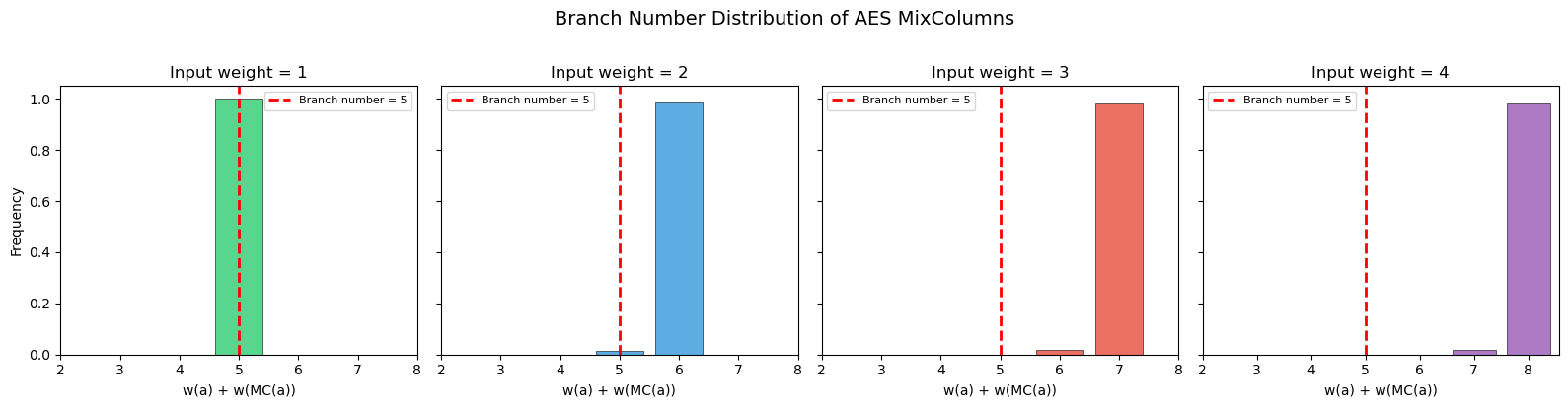
Minimum branch number observed per input weight:
  Weight 1: min = 5, mean = 5.00
  Weight 2: min = 5, mean = 5.99
  Weight 3: min = 5, mean = 6.98
  Weight 4: min = 7, mean = 7.98
Observation
Every input weight produces \(w(a) + w(\text{MixColumns}(a)) \geq 5\). This confirms the MDS property of the MixColumns matrix. Notice that for weight-1 inputs, the output always has full weight 4 (branch = 1 + 4 = 5), and for weight-4 inputs the branch is always \(\geq 5\) (output weight \(\geq 1\), which is guaranteed since MixColumns is invertible).
Experiment 2: Active S-Box Count vs Number of Rounds#
Show code cell source
import numpy as np
import matplotlib.pyplot as plt

# Known proven minimum active S-box counts for AES
rounds = np.arange(1, 11)
min_active = np.array([1, 5, 9, 25, 26, 30, 34, 50, 51, 55])

# Security thresholds
# For differential: need n * 6 >= 128 => n >= 22 active S-boxes
threshold_diff = np.ceil(128 / 6)  # ~22 S-boxes needed
# For linear: same, since max squared correlation is also 2^(-6)

fig, (ax1, ax2) = plt.subplots(1, 2, figsize=(14, 5))

# Left: Active S-boxes vs rounds
ax1.bar(rounds, min_active, color='#3498db', alpha=0.85, edgecolor='black',
        linewidth=0.5, zorder=3)
ax1.axhline(y=threshold_diff, color='red', linestyle='--', linewidth=2,
            label=f'128-bit security threshold ({int(threshold_diff)} S-boxes)',
            zorder=2)
ax1.set_xlabel('Number of AES Rounds', fontsize=12)
ax1.set_ylabel('Minimum Active S-boxes', fontsize=12)
ax1.set_title('Active S-boxes vs Rounds', fontsize=13)
ax1.set_xticks(rounds)
ax1.legend(fontsize=10)
ax1.grid(True, alpha=0.3, zorder=0)

# Annotate key values
for r, n in zip(rounds, min_active):
    ax1.text(r, n + 1.2, str(n), ha='center', fontsize=9, fontweight='bold')

# Right: Trail probability bound vs rounds
log_dp = -6 * min_active
ax2.plot(rounds, log_dp, 'o-', color='#e74c3c', linewidth=2, markersize=8,
         zorder=3, label='Diff/Linear trail bound')
ax2.axhline(y=-128, color='green', linestyle='--', linewidth=2,
            label='$2^{-128}$ threshold', zorder=2)
ax2.fill_between(rounds, log_dp, -128, where=(log_dp < -128),
                 alpha=0.15, color='green', label='Secure region')
ax2.fill_between(rounds, log_dp, -128, where=(log_dp >= -128),
                 alpha=0.15, color='red', label='Insecure region')
ax2.set_xlabel('Number of AES Rounds', fontsize=12)
ax2.set_ylabel('$\\log_2$(max trail probability)', fontsize=12)
ax2.set_title('Trail Probability Bound vs Rounds', fontsize=13)
ax2.set_xticks(rounds)
ax2.legend(fontsize=9, loc='lower left')
ax2.grid(True, alpha=0.3, zorder=0)

plt.tight_layout()
plt.savefig('aes_active_sboxes_vs_rounds.png', dpi=150, bbox_inches='tight')
plt.show()

print("Key observations:")
print(f"  4 rounds: 25 active S-boxes => DP <= 2^(-150), already secure")
print(f"  10 rounds (AES-128): 55 active S-boxes => DP <= 2^(-330)")
print(f"  Security margin: {float(abs(log_dp[9]) - 128):.0f} bits beyond threshold")

Key observations:
  4 rounds: 25 active S-boxes => DP <= 2^(-150), already secure
  10 rounds (AES-128): 55 active S-boxes => DP <= 2^(-330)
  Security margin: 202 bits beyond threshold
Experiment 3: AES S-Box Differential Uniformity and Linearity#
We visualize the DDT and LAT of the AES S-box and compare them with those of a random permutation.
Show code cell source
import numpy as np
import matplotlib.pyplot as plt

# Rebuild S-box (fresh imports)
def gf_mul(a, b, mod=0x11B):
    result = 0
    a, b = int(a), int(b)
    for _ in range(8):
        if b & 1:
            result ^= a
        a <<= 1
        if a & 0x100:
            a ^= mod
        b >>= 1
    return result

def gf_inv(a, mod=0x11B):
    if a == 0:
        return 0
    result = a
    for _ in range(6):
        result = gf_mul(result, result, mod)
        result = gf_mul(result, a, mod)
    result = gf_mul(result, result, mod)
    return result

def build_aes_sbox():
    sbox = np.zeros(256, dtype=np.uint8)
    aff_mat = np.array([
        [1,0,0,0,1,1,1,1],[1,1,0,0,0,1,1,1],[1,1,1,0,0,0,1,1],[1,1,1,1,0,0,0,1],
        [1,1,1,1,1,0,0,0],[0,1,1,1,1,1,0,0],[0,0,1,1,1,1,1,0],[0,0,0,1,1,1,1,1],
    ], dtype=np.uint8)
    aff_const = np.array([1,1,0,0,0,1,1,0], dtype=np.uint8)
    for i in range(256):
        inv = gf_inv(i)
        bits = np.array([(inv >> j) & 1 for j in range(8)], dtype=np.uint8)
        out_bits = (aff_mat @ bits + aff_const) % 2
        sbox[i] = sum(int(out_bits[j]) << j for j in range(8))
    return sbox

AES_SBOX = build_aes_sbox()

# Compute DDT
def compute_ddt(sbox):
    n = len(sbox)
    ddt = np.zeros((n, n), dtype=int)
    for x in range(n):
        for dx in range(n):
            dy = int(sbox[x]) ^ int(sbox[x ^ dx])
            ddt[dx, dy] += 1
    return ddt

DDT = compute_ddt(AES_SBOX)

# Also compute DDT for a random permutation
rng = np.random.default_rng(42)
random_perm = rng.permutation(256).astype(np.uint8)
DDT_rand = compute_ddt(random_perm)

fig, axes = plt.subplots(1, 3, figsize=(18, 5))

# Plot 1: AES DDT heatmap (first 64x64 for visibility)
im1 = axes[0].imshow(DDT[:64, :64], cmap='YlOrRd', aspect='equal',
                     interpolation='nearest', vmin=0, vmax=8)
axes[0].set_title('AES S-box DDT (first 64x64)', fontsize=11)
axes[0].set_xlabel('Output difference $\\Delta y$')
axes[0].set_ylabel('Input difference $\\Delta x$')
plt.colorbar(im1, ax=axes[0], shrink=0.8)

# Plot 2: Random permutation DDT heatmap
im2 = axes[1].imshow(DDT_rand[:64, :64], cmap='YlOrRd', aspect='equal',
                     interpolation='nearest', vmin=0, vmax=8)
axes[1].set_title('Random Permutation DDT (first 64x64)', fontsize=11)
axes[1].set_xlabel('Output difference $\\Delta y$')
axes[1].set_ylabel('Input difference $\\Delta x$')
plt.colorbar(im2, ax=axes[1], shrink=0.8)

# Plot 3: Distribution of DDT values (excluding dx=0)
aes_vals = DDT[1:, :].flatten()
rand_vals = DDT_rand[1:, :].flatten()

max_val = max(np.max(aes_vals), np.max(rand_vals))
bins = np.arange(0, max_val + 2) - 0.5

axes[2].hist(aes_vals, bins=bins, alpha=0.7, color='#3498db', density=True,
             label=f'AES S-box (max={np.max(aes_vals)})', edgecolor='black',
             linewidth=0.5)
axes[2].hist(rand_vals, bins=bins, alpha=0.5, color='#e74c3c', density=True,
             label=f'Random perm (max={np.max(rand_vals)})', edgecolor='black',
             linewidth=0.5)
axes[2].set_xlabel('DDT entry value')
axes[2].set_ylabel('Density')
axes[2].set_title('DDT Value Distribution', fontsize=11)
axes[2].legend(fontsize=9)
axes[2].set_xlim(-0.5, 12.5)

plt.tight_layout()
plt.savefig('aes_ddt_analysis.png', dpi=150, bbox_inches='tight')
plt.show()

print(f"AES S-box: max DDT entry = {np.max(DDT[1:, :])}, "
      f"differential uniformity = {np.max(DDT[1:, :])}")
print(f"Random permutation: max DDT entry = {np.max(DDT_rand[1:, :])}")
print(f"\nAES S-box is superior: max entry 4 vs {np.max(DDT_rand[1:, :])} for random.")
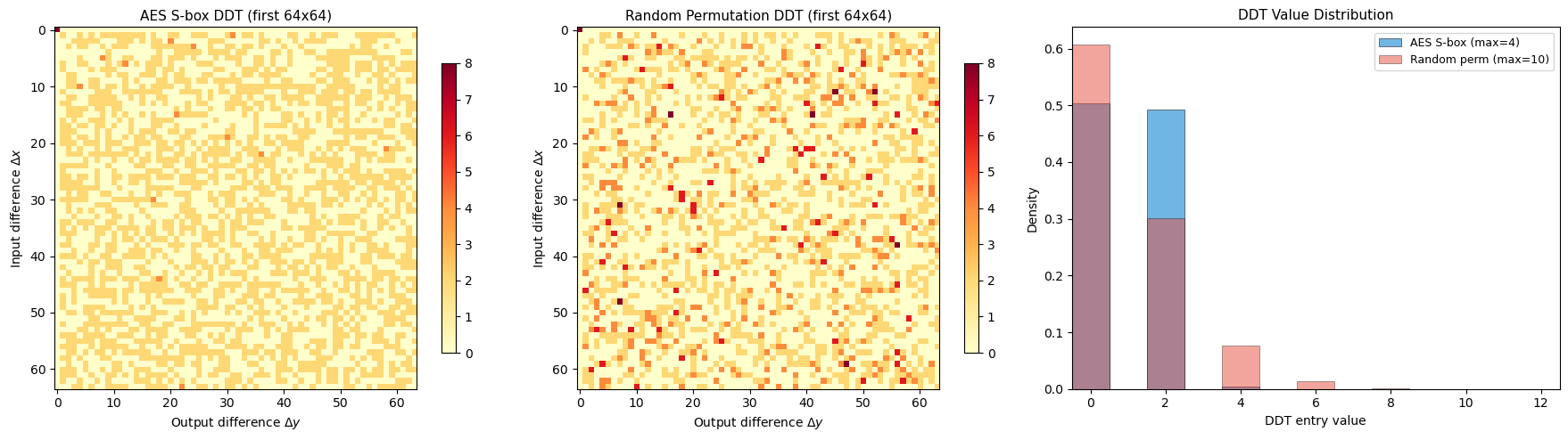
AES S-box: max DDT entry = 4, differential uniformity = 4
Random permutation: max DDT entry = 10

AES S-box is superior: max entry 4 vs 10 for random.
Experiment 4: Comparison – AES Resistance vs DES Resistance#
We compare the security margins of AES and DES against differential and linear cryptanalysis.
Show code cell source
import numpy as np
import matplotlib.pyplot as plt

# DES parameters
# DES: 16 rounds, 56-bit key, S-boxes are 6->4 bit
# Best differential: ~2^(-47) for 16 rounds (Biham-Shamir)
# Best linear: ~2^(-21) bias for 14 rounds -> needs 2^43 known plaintexts (Matsui)

des_rounds = np.arange(1, 17)
# Approximate DES min active S-boxes (from literature)
# DES has lower bounds of roughly: 1,?,3,5,7,10,12,14,16,18,19,20,21,22,23,25
# (approximate, not as clean as AES due to Feistel structure)
des_min_active = np.array([1, 1, 3, 5, 7, 10, 12, 14, 15, 17, 18, 19, 20, 21, 22, 25])
des_sbox_max_dp = 1/4  # = 2^(-2), DES S-boxes have higher max diff prob
des_log_dp = des_min_active * np.log2(des_sbox_max_dp)

# AES parameters
aes_rounds = np.arange(1, 11)
aes_min_active = np.array([1, 5, 9, 25, 26, 30, 34, 50, 51, 55])
aes_sbox_max_dp = 4/256  # = 2^(-6)
aes_log_dp = aes_min_active * np.log2(aes_sbox_max_dp)

fig, (ax1, ax2) = plt.subplots(1, 2, figsize=(14, 5))

# Plot 1: Active S-boxes comparison
ax1.plot(des_rounds, des_min_active, 's-', color='#e74c3c', linewidth=2,
         markersize=7, label='DES (16 rounds total)', zorder=3)
ax1.plot(aes_rounds, aes_min_active, 'o-', color='#3498db', linewidth=2,
         markersize=7, label='AES (10 rounds for AES-128)', zorder=3)
ax1.set_xlabel('Number of Rounds', fontsize=12)
ax1.set_ylabel('Minimum Active S-boxes', fontsize=12)
ax1.set_title('Active S-boxes: AES vs DES', fontsize=13)
ax1.legend(fontsize=10)
ax1.grid(True, alpha=0.3)

# Plot 2: Trail probability comparison
ax2.plot(des_rounds, des_log_dp, 's-', color='#e74c3c', linewidth=2,
         markersize=7, label='DES', zorder=3)
ax2.plot(aes_rounds, aes_log_dp, 'o-', color='#3498db', linewidth=2,
         markersize=7, label='AES', zorder=3)
ax2.axhline(y=-56, color='#e74c3c', linestyle=':', linewidth=1.5,
            alpha=0.7, label='DES key space ($2^{-56}$)')
ax2.axhline(y=-128, color='#3498db', linestyle=':', linewidth=1.5,
            alpha=0.7, label='AES-128 key space ($2^{-128}$)')
ax2.set_xlabel('Number of Rounds', fontsize=12)
ax2.set_ylabel('$\\log_2$(trail probability bound)', fontsize=12)
ax2.set_title('Differential Trail Probability: AES vs DES', fontsize=13)
ax2.legend(fontsize=9, loc='lower left')
ax2.grid(True, alpha=0.3)

plt.tight_layout()
plt.savefig('aes_vs_des_security.png', dpi=150, bbox_inches='tight')
plt.show()

print("Security comparison:")
print(f"  DES (16 rounds): trail prob <= 2^{float(des_log_dp[-1]):.0f} vs key space 2^(-56)")
print(f"    Security margin: {float(abs(des_log_dp[-1]) - 56):.0f} bits")
print(f"  AES (10 rounds): trail prob <= 2^{float(aes_log_dp[-1]):.0f} vs key space 2^(-128)")
print(f"    Security margin: {float(abs(aes_log_dp[-1]) - 128):.0f} bits")
print()
print("AES achieves a much larger security margin in fewer rounds,")
print("thanks to the wide trail strategy and superior S-box design.")
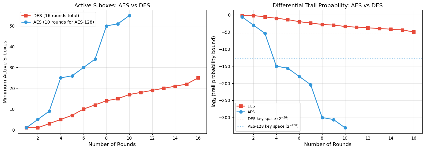
Security comparison:
  DES (16 rounds): trail prob <= 2^-50 vs key space 2^(-56)
    Security margin: -6 bits
  AES (10 rounds): trail prob <= 2^-330 vs key space 2^(-128)
    Security margin: 202 bits

AES achieves a much larger security margin in fewer rounds,
thanks to the wide trail strategy and superior S-box design.
Observation
The comparison reveals two key advantages of AES over DES:
Faster diffusion: AES reaches 25 active S-boxes in just 4 rounds, while DES needs all 16 rounds to reach a similar count. The SPN structure (SubBytes + ShiftRows + MixColumns) diffuses much faster than the Feistel structure.
Better S-box properties: The AES S-box has max differential probability \(2^{-6}\), while DES S-boxes have \(\sim 2^{-2}\). Each active S-box contributes three times more security in AES than in DES.
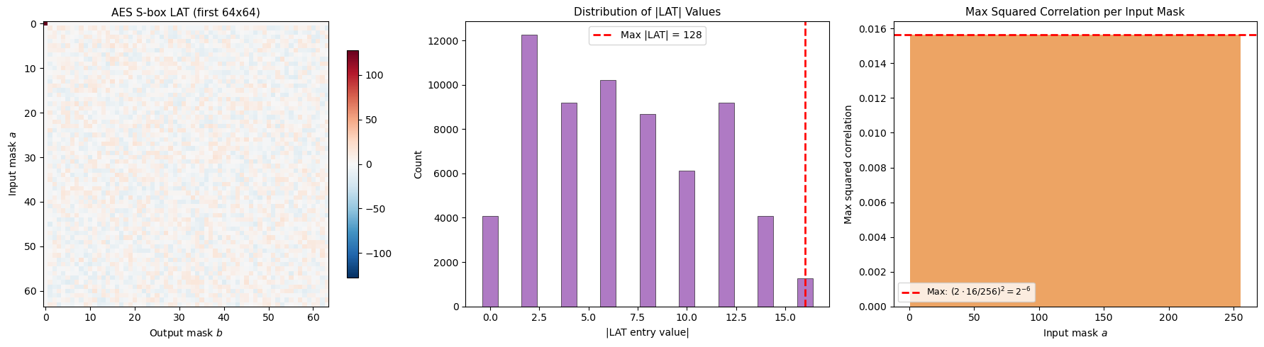
Experiment 5: LAT Visualization and Linearity Measurement#
Show code cell source
import numpy as np
import matplotlib.pyplot as plt

# Rebuild S-box
def gf_mul(a, b, mod=0x11B):
    result = 0
    a, b = int(a), int(b)
    for _ in range(8):
        if b & 1:
            result ^= a
        a <<= 1
        if a & 0x100:
            a ^= mod
        b >>= 1
    return result

def gf_inv(a, mod=0x11B):
    if a == 0:
        return 0
    result = a
    for _ in range(6):
        result = gf_mul(result, result, mod)
        result = gf_mul(result, a, mod)
    result = gf_mul(result, result, mod)
    return result

def build_aes_sbox():
    sbox = np.zeros(256, dtype=np.uint8)
    aff_mat = np.array([
        [1,0,0,0,1,1,1,1],[1,1,0,0,0,1,1,1],[1,1,1,0,0,0,1,1],[1,1,1,1,0,0,0,1],
        [1,1,1,1,1,0,0,0],[0,1,1,1,1,1,0,0],[0,0,1,1,1,1,1,0],[0,0,0,1,1,1,1,1],
    ], dtype=np.uint8)
    aff_const = np.array([1,1,0,0,0,1,1,0], dtype=np.uint8)
    for i in range(256):
        inv = gf_inv(i)
        bits = np.array([(inv >> j) & 1 for j in range(8)], dtype=np.uint8)
        out_bits = (aff_mat @ bits + aff_const) % 2
        sbox[i] = sum(int(out_bits[j]) << j for j in range(8))
    return sbox

AES_SBOX = build_aes_sbox()

# Compute LAT
def compute_lat(sbox):
    n = len(sbox)
    lat = np.zeros((n, n), dtype=int)
    for a in range(n):
        for b in range(n):
            count = 0
            for x in range(n):
                ax = bin(a & x).count('1') % 2
                bs = bin(b & int(sbox[x])).count('1') % 2
                if ax == bs:
                    count += 1
            lat[a, b] = count - n // 2
    return lat

print("Computing LAT (this takes a moment)...")
LAT = compute_lat(AES_SBOX)
print("Done.")

fig, axes = plt.subplots(1, 3, figsize=(18, 5))

# Plot 1: LAT heatmap
max_abs = np.max(np.abs(LAT))
im1 = axes[0].imshow(LAT[:64, :64], cmap='RdBu_r', aspect='equal',
                     interpolation='nearest', vmin=-max_abs, vmax=max_abs)
axes[0].set_title('AES S-box LAT (first 64x64)', fontsize=11)
axes[0].set_xlabel('Output mask $b$')
axes[0].set_ylabel('Input mask $a$')
plt.colorbar(im1, ax=axes[0], shrink=0.8)

# Plot 2: Distribution of |LAT| values
lat_abs = np.abs(LAT[1:, 1:]).flatten()  # Exclude a=0, b=0
unique_vals, counts = np.unique(lat_abs, return_counts=True)
axes[1].bar(unique_vals, counts, color='#9b59b6', alpha=0.8,
            edgecolor='black', linewidth=0.5)
axes[1].axvline(x=16, color='red', linestyle='--', linewidth=2,
                label=f'Max |LAT| = {int(max_abs)}')
axes[1].set_xlabel('|LAT entry value|')
axes[1].set_ylabel('Count')
axes[1].set_title('Distribution of |LAT| Values', fontsize=11)
axes[1].legend(fontsize=10)

# Plot 3: Squared correlation spectrum
# For each input mask a, find the max squared correlation
max_corr_per_mask = np.zeros(256)
for a in range(1, 256):
    max_bias = np.max(np.abs(LAT[a, 1:]))
    max_corr_per_mask[a] = (2 * max_bias / 256) ** 2

axes[2].bar(range(1, 256), max_corr_per_mask[1:], color='#e67e22', alpha=0.7,
            width=1.0)
axes[2].axhline(y=(2 * 16 / 256)**2, color='red', linestyle='--', linewidth=2,
                label=f'Max: $(2 \cdot  16/256)^2 = 2^{{-6}}$')
axes[2].set_xlabel('Input mask $a$')
axes[2].set_ylabel('Max squared correlation')
axes[2].set_title('Max Squared Correlation per Input Mask', fontsize=11)
axes[2].legend(fontsize=9)

plt.tight_layout()
plt.savefig('aes_lat_analysis.png', dpi=150, bbox_inches='tight')
plt.show()

print(f"Max |LAT| entry (a,b > 0): {np.max(np.abs(LAT[1:, 1:]))}")
print(f"Max linear bias: {np.max(np.abs(LAT[1:, 1:]))}/256 = 2^(-4)")
print(f"Max squared correlation: (2 * 2^(-4))^2 = 2^(-6)")
Computing LAT (this takes a moment)...
Done.
Max |LAT| entry (a,b > 0): 16
Max linear bias: 16/256 = 2^(-4)
Max squared correlation: (2 * 2^(-4))^2 = 2^(-6)
Observation
The LAT of the AES S-box shows a very uniform distribution of bias values, with the maximum absolute value being 16 (out of 256). This means the maximum linear bias is \(\varepsilon = 16/256 = 2^{-4}\) and the maximum squared correlation is \((2\varepsilon)^2 = 2^{-6}\). This matches the differential uniformity, a consequence of the S-box being based on the multiplicative inverse in \(\mathrm{GF}(2^8)\).
Experiment 6: MixColumns as an MDS Code – Submatrix Invertibility#
import numpy as np
from itertools import combinations

def gf_mul(a, b, mod=0x11B):
    result = 0
    a, b = int(a), int(b)
    for _ in range(8):
        if b & 1:
            result ^= a
        a <<= 1
        if a & 0x100:
            a ^= mod
        b >>= 1
    return result

MC = np.array([[2,3,1,1],[1,2,3,1],[1,1,2,3],[3,1,1,2]], dtype=int)

def gf_det_2x2(m):
    """Determinant of 2x2 matrix over GF(2^8)."""
    return gf_mul(m[0,0], m[1,1]) ^ gf_mul(m[0,1], m[1,0])

def gf_det_3x3(m):
    """Determinant of 3x3 matrix over GF(2^8) via cofactor expansion."""
    d = 0
    for j in range(3):
        # Minor: delete row 0, column j
        rows = [1, 2]
        cols = [c for c in range(3) if c != j]
        minor = np.array([[m[rows[0], cols[0]], m[rows[0], cols[1]]],
                          [m[rows[1], cols[0]], m[rows[1], cols[1]]]], dtype=int)
        cofactor = gf_mul(m[0, j], gf_det_2x2(minor))
        if j % 2 == 0:
            d ^= cofactor
        else:
            d ^= cofactor
    # Proper cofactor expansion in GF(2): all signs are +1 since -1 = 1
    return d

def gf_det_4x4(m):
    """Determinant of 4x4 matrix over GF(2^8) via cofactor expansion."""
    d = 0
    for j in range(4):
        rows = [1, 2, 3]
        cols = [c for c in range(4) if c != j]
        minor = np.array([[m[rows[r], cols[c]] for c in range(3)] for r in range(3)], dtype=int)
        cofactor = gf_mul(m[0, j], gf_det_3x3(minor))
        d ^= cofactor  # In GF(2), addition is XOR, so sign is irrelevant
    return d


print("Verifying MDS property: every square submatrix of MC is invertible")
print("=" * 65)
print()

# Check all 1x1 submatrices (trivial: all entries are nonzero)
all_nonzero = np.all(MC != 0)
print(f"1x1 submatrices (all entries nonzero): {all_nonzero}")
count_1x1 = 16

# Check all 2x2 submatrices
count_2x2 = 0
all_inv_2x2 = True
for rows in combinations(range(4), 2):
    for cols in combinations(range(4), 2):
        sub = np.array([[MC[rows[r], cols[c]] for c in range(2)] for r in range(2)], dtype=int)
        det = gf_det_2x2(sub)
        count_2x2 += 1
        if det == 0:
            all_inv_2x2 = False
            print(f"  SINGULAR 2x2: rows={rows}, cols={cols}, det={det}")
print(f"2x2 submatrices ({count_2x2} total, all invertible): {all_inv_2x2}")

# Check all 3x3 submatrices
count_3x3 = 0
all_inv_3x3 = True
for rows in combinations(range(4), 3):
    for cols in combinations(range(4), 3):
        sub = np.array([[MC[rows[r], cols[c]] for c in range(3)] for r in range(3)], dtype=int)
        det = gf_det_3x3(sub)
        count_3x3 += 1
        if det == 0:
            all_inv_3x3 = False
            print(f"  SINGULAR 3x3: rows={rows}, cols={cols}, det={det}")
print(f"3x3 submatrices ({count_3x3} total, all invertible): {all_inv_3x3}")

# Check the full 4x4 matrix
det_full = gf_det_4x4(MC)
print(f"4x4 (full matrix) determinant: {det_full} (nonzero = invertible): {det_full != 0}")

print()
if all_nonzero and all_inv_2x2 and all_inv_3x3 and (det_full != 0):
    print("==> ALL square submatrices are invertible.")
    print("==> MixColumns is an MDS matrix.")
    print("==> Branch number = 4 + 1 = 5 (maximum possible).")
else:
    print("==> MixColumns is NOT MDS (some submatrix is singular).")
Verifying MDS property: every square submatrix of MC is invertible
=================================================================

1x1 submatrices (all entries nonzero): True
2x2 submatrices (36 total, all invertible): True
3x3 submatrices (16 total, all invertible): True
4x4 (full matrix) determinant: 1 (nonzero = invertible): True

==> ALL square submatrices are invertible.
==> MixColumns is an MDS matrix.
==> Branch number = 4 + 1 = 5 (maximum possible).
24.5 Exercises#
Exercise 24.1 (Warm-up) Verify that the AES S-box is a permutation (bijection on \(\{0, 1, \ldots, 255\}\)). Then compute its algebraic degree – the degree of its polynomial representation over \(\mathrm{GF}(2^8)\).
Hint
Check bijectivity by verifying that len(set(AES_SBOX)) == 256. For the algebraic
degree, recall that the core of the AES S-box is \(x \mapsto x^{-1} = x^{254}\) in
\(\mathrm{GF}(2^8)\). Write \(254 = 11111110_2\) and count the number of 1-bits.
The algebraic degree of the power map \(x^d\) is the Hamming weight of \(d\), which
is \(\text{wt}(254) = 7\).
Exercise 24.2 (Applied) Construct a \(4 \times 4\) matrix over \(\mathrm{GF}(2^8)\) that is not MDS (branch number \(< 5\)). Find a specific nonzero input that achieves the minimum branch number, and explain why this makes the matrix unsuitable for use in a wide trail design.
Hint
Try the identity matrix \(I_4\). For input \((a, 0, 0, 0)\), the output is \((a, 0, 0, 0)\), giving branch number \(w(\text{in}) + w(\text{out}) = 1 + 1 = 2\). Alternatively, try a matrix with a singular \(2 \times 2\) submatrix (a zero determinant) – this allows two nonzero inputs to produce only one nonzero output.
Exercise 24.3 (Analysis) Show that for 2 rounds of AES, the minimum number of active S-boxes is exactly 5, by constructing a trail that achieves this bound. Specify the input difference pattern (which bytes are nonzero) at each stage: before SubBytes (round 1), after ShiftRows, after MixColumns, and before SubBytes (round 2).
Hint
Start with a single nonzero byte in position \((0, 0)\) of the state. After SubBytes, only byte \((0, 0)\) is active (1 active S-box). ShiftRows does not change this (row 0 is not shifted). MixColumns then spreads this single active byte to all 4 bytes of column 0, giving 4 active bytes entering round 2. Total: \(1 + 4 = 5\) active S-boxes.
Exercise 24.4 (Theory) Prove that the branch number of any invertible \(c \times c\) matrix over \(\mathrm{GF}(2^n)\) is at most \(c + 1\). Under what condition is equality achieved? (This is the MDS bound from coding theory.)
Hint
For any nonzero input \(a\) with \(w(a) = k\) nonzero components, the output \(\theta(a)\) has at most \(c\) nonzero components, so \(w(a) + w(\theta(a)) \leq k + c\). The minimum over \(k\) of \(k + c\) subject to \(k \geq 1\) is \(1 + c\). But this is not tight in general – the tighter argument uses the Singleton bound from coding theory. The matrix \([I | M]\) forms a generator matrix of a \([2c, c]\) code; the code is MDS iff every \(c \times c\) submatrix of \([I | M]\) is invertible, which is equivalent to every square submatrix of \(M\) being invertible.
Exercise 24.5 (Challenge) Implement a function that computes the exact branch number of an arbitrary \(4 \times 4\) matrix over \(\mathrm{GF}(2^4)\) (nibble-based, not byte-based) by exhaustive search over all \(2^{16} - 1\) nonzero inputs. Use this to find an MDS matrix over \(\mathrm{GF}(2^4)\) and verify its branch number is 5.
Hint
Use the irreducible polynomial \(x^4 + x + 1\) (0x13) for \(\mathrm{GF}(2^4)\). Iterate over all \(2^{16} - 1\) nonzero vectors \((a_0, a_1, a_2, a_3)\) where each \(a_i \in \{0, \ldots, 15\}\). Compute \(\theta(a)\) using matrix-vector multiplication over \(\mathrm{GF}(2^4)\), then find \(\min\{w(a) + w(\theta(a))\}\). A known MDS matrix over \(\mathrm{GF}(2^4)\) is: \(\begin{pmatrix} 1&1&1&4 \\ 1&4&1&1 \\ 4&1&1&1 \\ 1&1&4&1 \end{pmatrix}\).
24.6 Summary#
Concept |
Key Point |
|---|---|
Wide trail strategy |
Design philosophy ensuring minimum active S-boxes across rounds |
Branch number |
\(\mathcal{B}(\theta) = \min_{a \neq 0} \{ w(a) + w(\theta(a)) \}\); measures diffusion quality |
MixColumns branch number |
\(\mathcal{B} = 5\) (maximum for \(4 \times 4\) matrix = MDS) |
Active S-boxes (4 rounds) |
Minimum 25; gives trail probability \(\leq 2^{-150}\) |
Active S-boxes (10 rounds) |
Minimum 55; gives trail probability \(\leq 2^{-330}\) |
AES S-box differential uniformity |
4 (max DDT entry), giving \(p_{\max} = 2^{-6}\) |
AES S-box linearity |
Max bias \(2^{-4}\), max squared correlation \(2^{-6}\) |
Security margin |
Best known attack on full AES-128: \(2^{126.1}\) (biclique), essentially brute force |
AES vs DES |
AES achieves 202-bit margin over threshold; DES achieves only \(\sim\)6-bit margin |
Key Takeaway
The wide trail strategy transformed block cipher design from an art into a science. By proving lower bounds on active S-boxes through the branch number of the linear layer, Daemen and Rijmen showed that the security of AES against differential and linear cryptanalysis can be rigorously quantified. The resulting bounds (\(2^{-150}\) for 4 rounds, \(2^{-330}\) for 10 rounds) provide overwhelming security margins, making classical differential and linear attacks completely impractical against full AES.
Important caveat on trail bounds
A low differential/linear trail probability bound is necessary but not sufficient for security. It demonstrates resistance to basic single-trail attacks but does not account for clustering of multiple trails or other attack paradigms.
References#
Daemen, J. and Rijmen, V. (2002). The Design of Rijndael: AES – The Advanced Encryption Standard. Springer. [14]
Heys, H. M. (2002). A Tutorial on Linear and Differential Cryptanalysis. Cryptologia, 26(3), 189–221. [11]
Biham, E. and Shamir, A. (1991). Differential Cryptanalysis of DES-like Cryptosystems. Journal of Cryptology, 4(1), 3–72. [9]
Matsui, M. (1994). Linear Cryptanalysis Method for DES Cipher. EUROCRYPT ‘93, LNCS 765, 386–397. [10]
Bogdanov, A., Khovratovich, D., and Rechberger, C. (2011). Biclique Cryptanalysis of the Full AES. ASIACRYPT 2011, LNCS 7073, 344–371. [15]
NIST (2001). Advanced Encryption Standard (AES). FIPS Publication 197.