
Chapter 32: Structure of Point Groups on Elliptic Curves#
32.1 Introduction#
Every elliptic curve \(E\) over a finite field \(\mathbb{F}_p\) gives rise to a finite abelian group \(E(\mathbb{F}_p)\) consisting of all rational points together with the point at infinity \(\mathcal{O}\). Understanding the structure of this group is fundamental to elliptic curve cryptography: the security of protocols such as ECDH and ECDSA depends on \(E(\mathbb{F}_p)\) containing a large cyclic subgroup of prime order.
In this chapter we develop algorithms to:
Count the number of points on \(E(\mathbb{F}_p)\) (naive method and overview of Schoof’s algorithm).
Determine the group structure: is the group cyclic, or a product of two cyclic groups?
Find generators of the group.
Visualize how group orders distribute relative to \(p + 1\).
All implementations use only NumPy and matplotlib (plus the Python math module),
with explicit modular arithmetic throughout. We build on the elliptic curve point
addition from earlier chapters.
32.2 Elliptic Curve Arithmetic Foundations#
We represent an elliptic curve \(E: y^2 = x^3 + Ax + B\) over \(\mathbb{F}_p\) as a dictionary
{'A': A, 'B': B, 'p': p}. A point is either the tuple (x, y) with integer coordinates,
or the string 'O' denoting the point at infinity.
The following cell provides the complete arithmetic: point addition, scalar multiplication, and negation.
import numpy as np
import math

# ---------- Elliptic Curve Arithmetic over F_p ----------

def ec_curve(A, B, p):
    """Create an elliptic curve E: y^2 = x^3 + Ax + B over F_p.
    Checks the non-singularity condition 4A^3 + 27B^2 != 0 mod p."""
    disc = (4 * pow(A, 3, p) + 27 * pow(B, 2, p)) % p
    if disc == 0:
        raise ValueError(f"Singular curve: 4*{A}^3 + 27*{B}^2 = 0 mod {p}")
    return {'A': A % p, 'B': B % p, 'p': p}


def ec_neg(E, P):
    """Negate a point: -(x, y) = (x, -y)."""
    if P == 'O':
        return 'O'
    p = E['p']
    return (P[0], (-P[1]) % p)


def ec_add(E, P, Q):
    """Add two points on E(F_p) using the chord-and-tangent rule."""
    p = E['p']
    A = E['A']
    if P == 'O':
        return Q
    if Q == 'O':
        return P
    x1, y1 = P
    x2, y2 = Q
    if x1 == x2 and (y1 + y2) % p == 0:
        return 'O'
    if x1 == x2 and y1 == y2:
        # Point doubling
        num = (3 * x1 * x1 + A) % p
        den = (2 * y1) % p
    else:
        # General addition
        num = (y2 - y1) % p
        den = (x2 - x1) % p
    lam = (num * pow(den, -1, p)) % p
    x3 = (lam * lam - x1 - x2) % p
    y3 = (lam * (x1 - x3) - y1) % p
    return (x3, y3)


def ec_mul(E, k, P):
    """Scalar multiplication kP using double-and-add."""
    if k == 0 or P == 'O':
        return 'O'
    if k < 0:
        return ec_mul(E, -k, ec_neg(E, P))
    result = 'O'
    addend = P
    while k > 0:
        if k & 1:
            result = ec_add(E, result, addend)
        addend = ec_add(E, addend, addend)
        k >>= 1
    return result


def ec_on_curve(E, P):
    """Check whether P lies on E."""
    if P == 'O':
        return True
    x, y = P
    p = E['p']
    return (y * y - x * x * x - E['A'] * x - E['B']) % p == 0


# Quick test
E_test = ec_curve(1, 2, 11)
P_test = (3, 6)  # should be on y^2 = x^3 + x + 2 mod 11: 36 mod 11 = 3, 27+3+2=32, 32 mod 11 = 10... let's find a valid point

# Enumerate all points on E(F_11)
def ec_all_points(E):
    """Enumerate all points on E(F_p) by brute force."""
    p = E['p']
    A, B = E['A'], E['B']
    points = ['O']
    for x in range(p):
        rhs = (x * x * x + A * x + B) % p
        for y in range(p):
            if (y * y) % p == rhs:
                points.append((x, y))
    return points

pts = ec_all_points(E_test)
print(f"E(F_11) for y^2 = x^3 + x + 2 has {len(pts)} points.")
print("Points:", pts)
E(F_11) for y^2 = x^3 + x + 2 has 16 points.
Points: ['O', (1, 2), (1, 9), (2, 1), (2, 10), (4, 2), (4, 9), (5, 0), (6, 2), (6, 9), (7, 0), (8, 4), (8, 7), (9, 5), (9, 6), (10, 0)]
32.3 Naive Point Counting#
The simplest method for computing \(|E(\mathbb{F}_p)|\) is to loop over all \(x \in \mathbb{F}_p\) and check whether \(x^3 + Ax + B\) is a quadratic residue modulo \(p\). Using the Euler criterion, \(a\) is a square mod \(p\) if and only if \(a^{(p-1)/2} \equiv 1 \pmod{p}\) (or \(a = 0\)).
For each \(x\):
If \(x^3 + Ax + B = 0\): one point \((x, 0)\).
If \(x^3 + Ax + B\) is a non-zero square: two points \((x, y)\) and \((x, -y)\).
Otherwise: no points.
Add 1 for the point at infinity \(\mathcal{O}\).
Complexity
This algorithm has complexity \(O(p \log p)\) (one modular exponentiation per \(x\)-value), which is exponential in \(\log p\). It is unusable for primes of cryptographic size.
import numpy as np
import math

def naive_count(A, B, p):
    """Count |E(F_p)| for y^2 = x^3 + Ax + B by brute-force Euler criterion."""
    disc = (4 * pow(A, 3, p) + 27 * pow(B, 2, p)) % p
    if disc == 0:
        raise ValueError("Singular curve")
    count = 1  # point at infinity
    exp = (p - 1) // 2  # exponent for Euler criterion
    for x in range(p):
        rhs = (x * x * x + A * x + B) % p
        if rhs == 0:
            count += 1  # only (x, 0)
        elif pow(rhs, exp, p) == 1:
            count += 2  # (x, y) and (x, -y)
    return count

# Tests
print(f"E(F_11) for (A,B)=(1,2): |E| = {naive_count(1, 2, 11)}")
print(f"E(F_19) for (A,B)=(7,5): |E| = {naive_count(7, 5, 19)}")
print(f"E(F_193) for (A,B)=(11,3): |E| = {naive_count(11, 3, 193)}")
E(F_11) for (A,B)=(1,2): |E| = 16
E(F_19) for (A,B)=(7,5): |E| = 15
E(F_193) for (A,B)=(11,3): |E| = 194
Definition 32.1 (Order of a Point)
Let \(P \in E(\mathbb{F}_p)\) be a point. The order of \(P\), denoted \(\operatorname{ord}(P)\), is the smallest positive integer \(n\) such that \(nP = \mathcal{O}\) (the point at infinity). By Lagrange’s theorem, \(\operatorname{ord}(P)\) divides \(|E(\mathbb{F}_p)|\).
32.4 Computing the Order of a Point#
Given the group order \(N = |E(\mathbb{F}_p)|\), we know \(\operatorname{ord}(P) \mid N\). We can compute \(\operatorname{ord}(P)\) efficiently by starting with \(N\) and dividing out prime factors as long as the resulting multiple still sends \(P\) to \(\mathcal{O}\).
import numpy as np
import math

def trial_factor(n):
    """Return the prime factorisation of n as a list of (prime, exponent) pairs."""
    factors = []
    d = 2
    while d * d <= n:
        if n % d == 0:
            exp = 0
            while n % d == 0:
                n //= d
                exp += 1
            factors.append((d, exp))
        d += 1
    if n > 1:
        factors.append((n, 1))
    return factors


def point_order(E, P, N=None):
    """Compute the order of point P on curve E.
    If N (the group order) is known, uses the factor-and-divide method.
    Otherwise falls back to naive iteration."""
    if P == 'O':
        return 1
    if N is None:
        # Naive: iterate until we hit O
        Q = P
        for k in range(1, E['p'] + 2 * int(math.isqrt(E['p'])) + 2):
            if Q == 'O':
                return k
            Q = ec_add(E, Q, P)
        raise RuntimeError("Order not found (should not happen)")

    # Factor-and-divide: start with order = N, try to remove prime factors
    order = N
    for (q, e) in trial_factor(N):
        for _ in range(e):
            candidate = order // q
            if ec_mul(E, candidate, P) == 'O':
                order = candidate
            else:
                break
    return order


# Test: E(F_11) with (A,B)=(1,2), |E| = 16
E11 = ec_curve(1, 2, 11)
N11 = 16
pts11 = ec_all_points(E11)

print("Orders of all points on E(F_11):")
for P in pts11:
    print(f"  {str(P):>12s}  ->  order {point_order(E11, P, N11)}")
Orders of all points on E(F_11):
             O  ->  order 1
        (1, 2)  ->  order 4
        (1, 9)  ->  order 4
        (2, 1)  ->  order 8
       (2, 10)  ->  order 8
        (4, 2)  ->  order 8
        (4, 9)  ->  order 8
        (5, 0)  ->  order 2
        (6, 2)  ->  order 8
        (6, 9)  ->  order 8
        (7, 0)  ->  order 2
        (8, 4)  ->  order 4
        (8, 7)  ->  order 4
        (9, 5)  ->  order 8
        (9, 6)  ->  order 8
       (10, 0)  ->  order 2
32.5 The Structure Theorem#
Theorem 32.1 (Structure of \(E(\mathbb{F}_p)\))
Let \(E\) be an elliptic curve over \(\mathbb{F}_p\). Then:
(Hasse’s theorem) There exists an integer \(a\) with \(|a| \le 2\sqrt{p}\) such that \(|E(\mathbb{F}_p)| = p + 1 - a\). The integer \(a\) is called the trace of Frobenius.
(Structure theorem) There exist positive integers \(n_1, n_2\) with \(n_2 \mid n_1\) and \(n_2 \mid (p - 1)\) such that
\[ E(\mathbb{F}_p) \cong \mathbb{Z}/n_1\mathbb{Z} \times \mathbb{Z}/n_2\mathbb{Z}.\]In particular, \(|E(\mathbb{F}_p)| = n_1 \cdot n_2\).
The group is cyclic (i.e., \(n_2 = 1\)) if and only if it is generated by a single point. In practice, most elliptic curves over \(\mathbb{F}_p\) have cyclic point groups.
Definition 32.2 (Group Structure Decomposition)
The decomposition \(E(\mathbb{F}_p) \cong \mathbb{Z}/n_1\mathbb{Z} \times \mathbb{Z}/n_2\mathbb{Z}\) with \(n_2 \mid n_1\) and \(n_2 \mid \gcd(n_1, p-1)\) is called the invariant factor decomposition of the point group. When \(n_2 = 1\), the group is cyclic of order \(n_1 = |E(\mathbb{F}_p)|\).
32.6 Determining the Group Structure#
To determine \(n_1\) and \(n_2\), we use the following strategy:
Compute \(N = |E(\mathbb{F}_p)|\) (via naive counting for small \(p\)).
The maximal order among all points equals \(n_1\) (the exponent of the group).
Then \(n_2 = N / n_1\).
Verify that \(n_2 \mid n_1\) and \(n_2 \mid (p - 1)\).
For efficiency, we do not enumerate all points. Instead, we sample random points and track the least common multiple of their orders. When \(\operatorname{lcm}\) stabilises and divides \(N\) correctly, we have found \(n_1\).
import numpy as np
import math

def find_random_point(E, rng=None):
    """Find a random point on E(F_p) by trying random x-coordinates."""
    p = E['p']
    A, B = E['A'], E['B']
    if rng is None:
        rng = np.random.default_rng()
    while True:
        x = int(rng.integers(0, p))
        rhs = (x * x * x + A * x + B) % p
        if rhs == 0:
            return (x, 0)
        # Euler criterion
        if pow(rhs, (p - 1) // 2, p) == 1:
            # Tonelli-Shanks square root
            y = modular_sqrt(rhs, p)
            return (x, y)


def modular_sqrt(a, p):
    """Compute sqrt(a) mod p using the Tonelli-Shanks algorithm."""
    if a == 0:
        return 0
    if p == 2:
        return a % 2
    # Check that a is a QR
    if pow(a, (p - 1) // 2, p) != 1:
        raise ValueError(f"{a} is not a quadratic residue mod {p}")
    # Simple case: p = 3 mod 4
    if p % 4 == 3:
        return pow(a, (p + 1) // 4, p)
    # Tonelli-Shanks
    # Factor p-1 = Q * 2^S
    Q, S = p - 1, 0
    while Q % 2 == 0:
        Q //= 2
        S += 1
    # Find a quadratic non-residue
    z = 2
    while pow(z, (p - 1) // 2, p) != p - 1:
        z += 1
    M = S
    c = pow(z, Q, p)
    t = pow(a, Q, p)
    R = pow(a, (Q + 1) // 2, p)
    while True:
        if t == 1:
            return R
        # Find the least i such that t^(2^i) = 1
        i = 1
        temp = (t * t) % p
        while temp != 1:
            temp = (temp * temp) % p
            i += 1
        b = pow(c, 1 << (M - i - 1), p)
        M = i
        c = (b * b) % p
        t = (t * c) % p
        R = (R * b) % p


def group_structure(E, N=None):
    """Determine the group structure of E(F_p).
    Returns (n1, n2) where E(F_p) = Z/n1 x Z/n2, n2 | n1.
    If N is not provided, computes it via naive counting."""
    p = E['p']
    if N is None:
        N = naive_count(E['A'], E['B'], p)

    # Strategy: find the exponent n1 (max order of any element)
    # by computing lcm of orders of random points.
    rng = np.random.default_rng(42)
    exponent = 1
    # For small p, we can enumerate all points
    if p < 10000:
        pts = ec_all_points(E)
        for P in pts:
            if P == 'O':
                continue
            ord_P = point_order(E, P, N)
            exponent = math.lcm(exponent, ord_P)
    else:
        # Sample random points
        stable_count = 0
        for _ in range(200):
            P = find_random_point(E, rng)
            ord_P = point_order(E, P, N)
            new_exp = math.lcm(exponent, ord_P)
            if new_exp == exponent:
                stable_count += 1
                if stable_count > 20:
                    break
            else:
                exponent = new_exp
                stable_count = 0

    n1 = exponent
    n2 = N // n1
    return (n1, n2)


# Test
E11 = ec_curve(1, 2, 11)
n1, n2 = group_structure(E11, 16)
print(f"E(F_11) for y^2 = x^3 + x + 2:  Z/{n1} x Z/{n2}")
print(f"  n2 | n1: {n1 % n2 == 0},  n2 | (p-1): {(11 - 1) % n2 == 0}")

E19 = ec_curve(7, 5, 19)
N19 = naive_count(7, 5, 19)
n1, n2 = group_structure(E19, N19)
print(f"\nE(F_19) for y^2 = x^3 + 7x + 5:  Z/{n1} x Z/{n2}  (|E| = {N19})")
print(f"  n2 | n1: {n1 % n2 == 0}")
E(F_11) for y^2 = x^3 + x + 2:  Z/8 x Z/2
  n2 | n1: True,  n2 | (p-1): True

E(F_19) for y^2 = x^3 + 7x + 5:  Z/15 x Z/1  (|E| = 15)
  n2 | n1: True
Definition 32.3 (Torsion Subgroup)
For a positive integer \(m\), the \(m\)-torsion subgroup of \(E(\mathbb{F}_p)\) is
If \(\gcd(m, p) = 1\), then \(E[m] \cong \mathbb{Z}/m\mathbb{Z} \times \mathbb{Z}/m\mathbb{Z}\) when considered over the algebraic closure \(\overline{\mathbb{F}_p}\). Over \(\mathbb{F}_p\) itself, \(E[m]\) may be smaller – it is a subgroup of \(\mathbb{Z}/m\mathbb{Z} \times \mathbb{Z}/m\mathbb{Z}\).
The \(m\)-torsion subgroup plays a central role in Schoof’s algorithm: by computing the action of the Frobenius endomorphism on \(E[\ell]\) for small primes \(\ell\), one can determine \(a \bmod \ell\) and then reconstruct \(a\) via the Chinese Remainder Theorem.
32.7 Finding Generators#
Once we know the structure \(E(\mathbb{F}_p) \cong \mathbb{Z}/n_1\mathbb{Z} \times \mathbb{Z}/n_2\mathbb{Z}\), we need to find generators: a point \(P_1\) of order \(n_1\) and (if \(n_2 > 1\)) a point \(P_2\) of order \(n_2\) such that \(P_2 \notin \langle P_1 \rangle\).
import numpy as np
import math

def find_generators(E, N=None):
    """Find generators of E(F_p).
    Returns (n1, n2, P1, P2) where:
      - P1 has order n1 (generates the large cyclic factor)
      - P2 has order n2 (generates the small cyclic factor, or 'O' if n2=1)
    """
    p = E['p']
    if N is None:
        N = naive_count(E['A'], E['B'], p)

    n1, n2 = group_structure(E, N)

    # Find a point of order n1
    P1 = None
    pts = ec_all_points(E) if p < 10000 else None

    if pts is not None:
        for P in pts:
            if P == 'O':
                continue
            if point_order(E, P, N) == n1:
                P1 = P
                break
    else:
        rng = np.random.default_rng(123)
        while P1 is None:
            P = find_random_point(E, rng)
            # Scale P so that its order is n1
            ord_P = point_order(E, P, N)
            if ord_P == n1:
                P1 = P

    if n2 == 1:
        return (n1, n2, P1, 'O')

    # Find a point of order n2 not in <P1>
    # Strategy: find point Q, compute Q' = (N/n2)*Q which has order dividing n2.
    # Check Q' is not in <P1> by verifying it's not a multiple of (n1/n2)*P1.
    P2 = None
    if pts is not None:
        # Generate the subgroup <P1>
        subgroup_P1 = set()
        R = 'O'
        for k in range(n1):
            subgroup_P1.add(R if R == 'O' else R)
            R = ec_add(E, R, P1)

        for P in pts:
            if P == 'O' or P in subgroup_P1:
                continue
            ord_P = point_order(E, P, N)
            if ord_P % n2 == 0:
                # Scale to get order exactly n2
                Q = ec_mul(E, ord_P // n2, P)
                if Q != 'O' and Q not in subgroup_P1:
                    P2 = Q
                    break

    if P2 is None:
        P2 = 'O'  # fallback

    return (n1, n2, P1, P2)


def is_cyclic(E, N=None):
    """Check whether E(F_p) is cyclic."""
    if N is None:
        N = naive_count(E['A'], E['B'], E['p'])
    n1, n2 = group_structure(E, N)
    return n2 == 1


# Test with E(F_11), y^2 = x^3 + x + 2, |E| = 16, structure Z/8 x Z/2
E11 = ec_curve(1, 2, 11)
n1, n2, P1, P2 = find_generators(E11, 16)
print(f"Structure: Z/{n1} x Z/{n2}")
print(f"Generator P1 = {P1}, order = {point_order(E11, P1, 16)}")
print(f"Generator P2 = {P2}, order = {point_order(E11, P2, 16) if P2 != 'O' else 1}")
print(f"Cyclic? {is_cyclic(E11, 16)}")

# Test with E(F_19), y^2 = x^3 + 7x + 5 (cyclic of order 15)
E19 = ec_curve(7, 5, 19)
N19 = naive_count(7, 5, 19)
n1, n2, P1, P2 = find_generators(E19, N19)
print(f"\nE(F_19): Z/{n1} x Z/{n2}")
print(f"Generator P1 = {P1}")
print(f"Cyclic? {is_cyclic(E19, N19)}")
Structure: Z/8 x Z/2
Generator P1 = (2, 1), order = 8
Generator P2 = (5, 0), order = 2
Cyclic? False

E(F_19): Z/15 x Z/1
Generator P1 = (0, 9)
Cyclic? True
32.8 Verification: Enumerating Generated Points#
For small primes, we can verify our generators are correct by checking that every point on the curve can be expressed as \(a \cdot P_1 + b \cdot P_2\) for some integers \(a, b\).
import numpy as np
import math

def verify_generators(E, n1, n2, P1, P2):
    """Verify that P1, P2 generate the full group E(F_p)."""
    generated = set()
    for a in range(n1):
        aP1 = ec_mul(E, a, P1)
        for b in range(n2):
            if n2 == 1:
                pt = aP1
            else:
                bP2 = ec_mul(E, b, P2)
                pt = ec_add(E, aP1, bP2)
            generated.add(pt)

    actual = set()
    for P in ec_all_points(E):
        actual.add(P)

    return generated == actual

# E(F_11): Z/8 x Z/2
E11 = ec_curve(1, 2, 11)
n1, n2, P1, P2 = find_generators(E11, 16)
ok = verify_generators(E11, n1, n2, P1, P2)
print(f"E(F_11): generators verified = {ok}")

# E(F_19): Z/15 (cyclic)
E19 = ec_curve(7, 5, 19)
N19 = naive_count(7, 5, 19)
n1, n2, P1, P2 = find_generators(E19, N19)
ok = verify_generators(E19, n1, n2, P1, P2)
print(f"E(F_19): generators verified = {ok}")
E(F_11): generators verified = True
E(F_19): generators verified = True
32.9 Experiment: Group Structures for Various Curves and Primes#
Let us survey the group structure of \(E(\mathbb{F}_p)\) for several curves and primes.
import numpy as np
import math

def sieve_primes(limit):
    """Return a list of primes up to limit using the Sieve of Eratosthenes."""
    is_prime = np.ones(limit + 1, dtype=bool)
    is_prime[:2] = False
    for i in range(2, int(np.sqrt(limit)) + 1):
        if is_prime[i]:
            is_prime[i*i::i] = False
    return list(np.where(is_prime)[0])

# Test curves
test_cases = [
    (1, 2, 11),
    (7, 5, 19),
    (1, 1, 19),
    (11, 3, 193),
    (12, 5, 271),
    (199, 272, 1013),
    (1, 3, 7927),
    (2, 7, 997),
    (3, 5, 1009),
    (5, 11, 2003),
]

print(f"{'Curve (A,B)':>14s}  {'p':>6s}  {'|E|':>6s}  {'Hasse a':>8s}  {'Structure':>16s}  {'Cyclic':>7s}")
print("-" * 70)
for A, B, p in test_cases:
    try:
        E = ec_curve(A, B, p)
        N = naive_count(A, B, p)
        a_trace = p + 1 - N
        n1, n2 = group_structure(E, N)
        cyc = "yes" if n2 == 1 else "no"
        struct = f"Z/{n1}" if n2 == 1 else f"Z/{n1} x Z/{n2}"
        print(f"  ({int(A):>3d},{int(B):>3d})    {int(p):>6d}  {int(N):>6d}  {int(a_trace):>8d}  {struct:>16s}  {cyc:>7s}")
    except ValueError as e:
        print(f"  ({int(A):>3d},{int(B):>3d})    {int(p):>6d}  -- singular --")
   Curve (A,B)       p     |E|   Hasse a         Structure   Cyclic
----------------------------------------------------------------------
  (  1,  2)        11      16        -4         Z/8 x Z/2       no
  (  7,  5)        19      15         5              Z/15      yes
  (  1,  1)        19      21        -1              Z/21      yes
  ( 11,  3)       193     194         0             Z/194      yes
  ( 12,  5)       271     289       -17             Z/289      yes
  (199,272)      1013    1035       -21            Z/1035      yes
  (  1,  3)      7927    7925         3            Z/7925      yes
  (  2,  7)       997    1045       -47            Z/1045      yes
  (  3,  5)      1009    1023       -13            Z/1023      yes
( 5, 11) 2003 1974 30 Z/1974 yes
Observation
Most curves in the table above are cyclic (\(n_2 = 1\)). The non-cyclic cases correspond to group orders that have a non-trivial common factor with \(p - 1\), and even then the group is often cyclic. Non-cyclic groups are the exception, not the rule.
32.10 Experiment: Distribution of Group Orders (Hasse Histogram)#
Hasse’s theorem tells us \(|E(\mathbb{F}_p)| \in [p + 1 - 2\sqrt{p},\; p + 1 + 2\sqrt{p}]\). Let us fix a prime \(p\) and vary the curve parameters \((A, B)\) to see how the group order distributes within this interval.
Show code cell source
import numpy as np
import matplotlib.pyplot as plt
import math

p = 499  # a moderate prime
orders = []

for A in range(1, p):
    for B in range(1, min(p, 50)):  # sample B values to keep runtime manageable
        disc = (4 * pow(A, 3, p) + 27 * pow(B, 2, p)) % p
        if disc == 0:
            continue
        N = naive_count(A, B, p)
        orders.append(N)

orders = np.array(orders)
hasse_low = p + 1 - 2 * int(math.isqrt(p)) - 2
hasse_high = p + 1 + 2 * int(math.isqrt(p)) + 2

fig, ax = plt.subplots(figsize=(10, 5))
bins = np.arange(hasse_low, hasse_high + 2)
ax.hist(orders, bins=bins, color='steelblue', edgecolor='white', alpha=0.85)
ax.axvline(p + 1, color='red', linestyle='--', linewidth=2, label=f'$p + 1 = {p + 1}$')
ax.axvline(p + 1 - 2 * math.isqrt(p), color='orange', linestyle=':', linewidth=1.5,
           label=f'$p+1-2\\sqrt{{p}} \\approx {p + 1 - 2 * math.isqrt(p)}$')
ax.axvline(p + 1 + 2 * math.isqrt(p), color='orange', linestyle=':', linewidth=1.5,
           label=f'$p+1+2\\sqrt{{p}} \\approx {p + 1 + 2 * math.isqrt(p)}$')
ax.set_xlabel('Group order $|E(\\mathbb{F}_p)|$', fontsize=12)
ax.set_ylabel('Frequency', fontsize=12)
ax.set_title(f'Distribution of group orders for $p = {p}$', fontsize=14)
ax.legend(fontsize=10)
plt.tight_layout()
plt.savefig('ch32_hasse_histogram.png', dpi=150, bbox_inches='tight')
plt.show()

print(f"\nSampled {len(orders)} curves over F_{p}")
print(f"Order range: [{orders.min()}, {orders.max()}]")
print(f"Hasse bounds: [{p + 1 - 2 * math.isqrt(p)}, {p + 1 + 2 * math.isqrt(p)}]")
print(f"Mean order: {float(orders.mean()):.1f}  (p+1 = {p+1})")
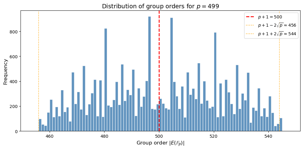
Sampled 24342 curves over F_499
Order range: [456, 544]
Hasse bounds: [456, 544]
Mean order: 500.1  (p+1 = 500)
Observation
The distribution of \(|E(\mathbb{F}_p)|\) is concentrated around \(p + 1\) and has a characteristic semicircular shape (related to the Sato-Tate distribution for the normalised trace \(a / (2\sqrt{p})\)). The histogram above illustrates this directly: most group orders cluster near \(p + 1\).
32.11 Experiment: Cyclic vs Non-Cyclic Groups#
How often is \(E(\mathbb{F}_p)\) cyclic? We survey many random curves for a fixed prime.
import numpy as np
import matplotlib.pyplot as plt
import math

def survey_cyclic(p, num_curves=500, seed=42):
    """Survey random curves over F_p and report cyclic vs non-cyclic counts."""
    rng = np.random.default_rng(seed)
    cyclic_count = 0
    noncyclic_count = 0
    noncyclic_examples = []

    attempts = 0
    while cyclic_count + noncyclic_count < num_curves and attempts < 5 * num_curves:
        attempts += 1
        A = int(rng.integers(1, p))
        B = int(rng.integers(1, p))
        disc = (4 * pow(A, 3, p) + 27 * pow(B, 2, p)) % p
        if disc == 0:
            continue
        try:
            E = ec_curve(A, B, p)
            N = naive_count(A, B, p)
            n1, n2 = group_structure(E, N)
            if n2 == 1:
                cyclic_count += 1
            else:
                noncyclic_count += 1
                if len(noncyclic_examples) < 5:
                    noncyclic_examples.append((A, B, N, n1, n2))
        except (ValueError, ZeroDivisionError):
            continue

    return cyclic_count, noncyclic_count, noncyclic_examples


# Survey for several primes
primes_survey = [101, 199, 307, 499, 701]
results = []

print(f"{'p':>6s}  {'Curves':>7s}  {'Cyclic':>7s}  {'Non-cyc':>8s}  {'% Cyclic':>9s}")
print("-" * 45)
for p in primes_survey:
    cyc, ncyc, examples = survey_cyclic(p, num_curves=300)
    total = cyc + ncyc
    pct = 100 * cyc / total if total > 0 else 0
    results.append((p, cyc, ncyc, pct))
    print(f"{int(p):>6d}  {int(total):>7d}  {int(cyc):>7d}  {int(ncyc):>8d}  {float(pct):>8.1f}%")
    if examples:
        print(f"         Non-cyclic examples: {examples[:2]}")
     p   Curves   Cyclic   Non-cyc   % Cyclic
---------------------------------------------
   101      300      254        46      84.7%
         Non-cyclic examples: [(79, 65, 84, 42, 2), (55, 45, 84, 42, 2)]
   199      300      234        66      78.0%
         Non-cyclic examples: [(18, 154, 184, 92, 2), (130, 87, 224, 112, 2)]
   307      300      242        58      80.7%
         Non-cyclic examples: [(167, 136, 288, 144, 2), (263, 254, 284, 142, 2)]
   499      300      250        50      83.3%
         Non-cyclic examples: [(419, 225, 480, 240, 2), (250, 185, 522, 174, 3)]
   701      300      254        46      84.7%
         Non-cyclic examples: [(65, 389, 700, 70, 10), (622, 45, 684, 342, 2)]
Show code cell source
import numpy as np
import matplotlib.pyplot as plt

# Bar chart: cyclic vs non-cyclic
primes_labels = [str(r[0]) for r in results]
cyc_counts = [r[1] for r in results]
ncyc_counts = [r[2] for r in results]

x_pos = np.arange(len(primes_labels))
width = 0.35

fig, ax = plt.subplots(figsize=(8, 5))
bars1 = ax.bar(x_pos - width/2, cyc_counts, width, label='Cyclic', color='steelblue')
bars2 = ax.bar(x_pos + width/2, ncyc_counts, width, label='Non-cyclic', color='salmon')

ax.set_xlabel('Prime $p$', fontsize=12)
ax.set_ylabel('Number of curves', fontsize=12)
ax.set_title('Cyclic vs Non-Cyclic Point Groups', fontsize=14)
ax.set_xticks(x_pos)
ax.set_xticklabels(primes_labels)
ax.legend(fontsize=11)

# Add percentage labels
for i, (c, n) in enumerate(zip(cyc_counts, ncyc_counts)):
    total = c + n
    ax.text(i - width/2, c + 3, f'{float(100*c/total):.0f}%', ha='center', fontsize=9)

plt.tight_layout()
plt.savefig('ch32_cyclic_vs_noncyclic.png', dpi=150, bbox_inches='tight')
plt.show()
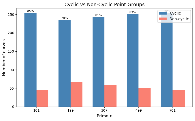
Observation
The vast majority of elliptic curves over \(\mathbb{F}_p\) have cyclic point groups. Non-cyclic groups (where \(E(\mathbb{F}_p) \cong \mathbb{Z}/n_1 \times \mathbb{Z}/n_2\) with \(n_2 > 1\)) do occur, but cyclic groups are much more common for random curves over large fields. Intuitively, the constraint \(n_2 \mid \gcd(n_1, p - 1)\) is hard to satisfy when \(p\) is large and the group order is essentially random within the Hasse interval. This is good news for cryptography: randomly chosen curves almost always yield the cyclic groups needed for ECDLP-based protocols.
32.12 Schoof’s Algorithm: Overview#
The naive counting method is \(O(p)\), which is exponential in \(\log p\). For cryptographic primes (\(p \approx 2^{256}\)), this is completely infeasible.
Schoof’s algorithm (1985) computes \(|E(\mathbb{F}_p)|\) in polynomial time \(O(\log^8 p)\) (or better with the Schoof-Elkies-Atkin improvements).
The key idea:
The Frobenius endomorphism \(\phi: (x, y) \mapsto (x^p, y^p)\) satisfies \(\phi^2 - a\phi + p = 0\) on \(E\), where \(a = p + 1 - |E(\mathbb{F}_p)|\).
For each small prime \(\ell\), restrict to the \(\ell\)-torsion subgroup \(E[\ell]\) and compute \(a \bmod \ell\) by checking which value makes the characteristic equation hold.
Use the Chinese Remainder Theorem to reconstruct \(a\) from its residues modulo \(\ell_1, \ell_2, \ldots, \ell_k\), where \(\prod \ell_i > 4\sqrt{p}\).
We illustrate the principle with a small example.
import numpy as np
import math

def extended_gcd(a, b):
    """Extended Euclidean algorithm: returns (g, x, y) such that a*x + b*y = g."""
    if a == 0:
        return b, 0, 1
    g, x, y = extended_gcd(b % a, a)
    return g, y - (b // a) * x, x


def crt(residues, moduli):
    """Chinese Remainder Theorem: solve x = r_i mod m_i."""
    if len(residues) == 0:
        return 0, 1
    x, M = residues[0], moduli[0]
    for r, m in zip(residues[1:], moduli[1:]):
        g, p_inv, _ = extended_gcd(M, m)
        if (r - x) % g != 0:
            raise ValueError("No solution")
        lcm = M * m // g
        x = (x + M * ((r - x) // g) * p_inv) % lcm
        M = lcm
    return x, M


def schoof_demo(A, B, p):
    """Demonstrate Schoof's approach for small p.
    For each small prime ell, find a point of order ell (if it exists),
    determine a mod ell by testing the Frobenius relation, then reconstruct a via CRT."""
    E = ec_curve(A, B, p)
    N_actual = naive_count(A, B, p)
    a_actual = p + 1 - N_actual
    hasse_bound = 2 * math.isqrt(p) + 1

    print(f"Curve: y^2 = x^3 + {A}x + {B} over F_{p}")
    print(f"Actual: |E| = {N_actual}, trace a = {a_actual}")
    print(f"Hasse bound: |a| <= {2 * math.isqrt(p)}")
    print(f"Need product of primes > {4 * math.isqrt(p)}")
    print()

    # Find torsion points and determine a mod ell
    pts = ec_all_points(E)
    residues = []
    moduli = []
    product = 1

    small_primes = sieve_primes(50)

    for ell in small_primes:
        if ell == p:
            continue
        if product > 4 * math.isqrt(p):
            break

        # Find a point of order ell
        torsion_pt = None
        for Q in pts:
            if Q == 'O':
                continue
            ord_Q = point_order(E, Q, N_actual)
            if ord_Q % ell == 0:
                # Scale to get order exactly ell
                torsion_pt = ec_mul(E, ord_Q // ell, Q)
                if torsion_pt != 'O':
                    break

        if torsion_pt is None:
            continue

        # Determine a mod ell by testing: phi^2(P) + p*P = a * phi(P)
        # In F_p, Frobenius is the identity on coordinates, so phi(P) = P
        # The relation becomes: P + p*P = a*P, i.e. (1+p)*P = a*P
        # So a = 1 + p mod ord(torsion_pt) = 1 + p mod ell
        # Actually for points in E(F_p), Frobenius fixes them,
        # so we directly compute: for which a_test does (p+1-a_test)*P = O?
        a_mod_ell = None
        for a_test in range(ell):
            if ec_mul(E, (p + 1 - a_test) % ell, torsion_pt) == 'O':
                a_mod_ell = a_test
                break

        if a_mod_ell is not None:
            residues.append(a_mod_ell)
            moduli.append(ell)
            product *= ell
            print(f"  ell = {int(ell):>3d}:  torsion point = {str(torsion_pt):>15s},  "
                  f"a = {a_mod_ell} mod {ell}  (actual: {a_actual % ell})")

    # Reconstruct a via CRT
    if len(residues) > 0:
        a_crt, M = crt(residues, moduli)
        # Adjust to the range [-2sqrt(p), 2sqrt(p)]
        if a_crt > M // 2:
            a_crt -= M
        print(f"\nCRT reconstruction: a = {a_crt} (mod {M})")
        print(f"Recovered |E| = p + 1 - a = {p + 1 - a_crt}")
        print(f"Correct: {p + 1 - a_crt == N_actual}")
    else:
        print("Could not find enough torsion points.")


schoof_demo(1, 1, 19)
Curve: y^2 = x^3 + 1x + 1 over F_19
Actual: |E| = 21, trace a = -1
Hasse bound: |a| <= 8
Need product of primes > 16

  ell =   3:  torsion point =          (2, 7),  a = 2 mod 3  (actual: 2)
  ell =   7:  torsion point =         (15, 3),  a = 6 mod 7  (actual: 6)

CRT reconstruction: a = -1 (mod 21)
Recovered |E| = p + 1 - a = 21
Correct: True
import numpy as np
import math

# Another example with a moderate prime whose group order has many small prime factors
# We pick (A, B, p) = (1, 9, 211) where |E| = 210 = 2 * 3 * 5 * 7,
# giving plenty of small-prime torsion for the CRT reconstruction.
print("=" * 60)
schoof_demo(1, 9, 211)
============================================================
Curve: y^2 = x^3 + 1x + 9 over F_211
Actual: |E| = 210, trace a = 2
Hasse bound: |a| <= 28
Need product of primes > 56

  ell =   2:  torsion point =        (112, 0),  a = 0 mod 2  (actual: 0)
  ell =   3:  torsion point =       (72, 131),  a = 2 mod 3  (actual: 2)
  ell =   5:  torsion point =       (126, 81),  a = 2 mod 5  (actual: 2)
  ell =   7:  torsion point =       (116, 26),  a = 2 mod 7  (actual: 2)

CRT reconstruction: a = 2 (mod 210)
Recovered |E| = p + 1 - a = 210
Correct: True
Important caveat
The demonstration above is not a true implementation of Schoof’s algorithm. The real algorithm works with division polynomials in the polynomial ring \(\mathbb{F}_p[x]\) to compute the action of the Frobenius on \(E[\ell]\) without enumerating individual \(\ell\)-torsion points. This is what makes it polynomial-time. Our demonstration merely illustrates the CRT-based reconstruction principle.
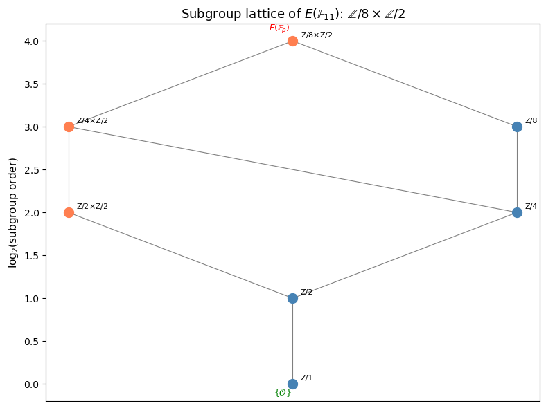
32.13 Visualising the Subgroup Lattice#
The subgroup lattice of a finite abelian group shows the inclusion relationships between all subgroups. For a cyclic group \(\mathbb{Z}/n\mathbb{Z}\), the subgroup lattice is isomorphic to the divisor lattice of \(n\). For \(\mathbb{Z}/n_1 \times \mathbb{Z}/n_2\), the structure is richer.
Show code cell source
import numpy as np
import matplotlib.pyplot as plt
import math

def divisors(n):
    """Return sorted list of divisors of n."""
    divs = []
    for d in range(1, int(math.isqrt(n)) + 1):
        if n % d == 0:
            divs.append(d)
            if d != n // d:
                divs.append(n // d)
    return sorted(divs)


def subgroup_orders(n1, n2):
    """Compute all possible subgroup orders for Z/n1 x Z/n2.
    A subgroup of Z/n1 x Z/n2 has the form Z/d1 x Z/d2 where d1 | n1, d2 | n2, d2 | d1.
    Returns list of (d1, d2) pairs and the total order d1*d2."""
    subgroups = []
    for d1 in divisors(n1):
        for d2 in divisors(n2):
            if d2 <= d1 and d1 % d2 == 0:
                subgroups.append((d1, d2, d1 * d2))
    return subgroups


def plot_subgroup_lattice(n1, n2, title=""):
    """Plot the subgroup lattice of Z/n1 x Z/n2."""
    subs = subgroup_orders(n1, n2)

    # Group by total order for y-position
    order_to_subs = {}
    for d1, d2, total in subs:
        order_to_subs.setdefault(total, []).append((d1, d2))

    sorted_orders = sorted(order_to_subs.keys())
    # Use log scale for y positions
    y_map = {}
    for i, order in enumerate(sorted_orders):
        y_map[order] = np.log2(order) if order > 0 else 0

    # Assign positions
    positions = {}  # (d1, d2) -> (x, y)
    for order in sorted_orders:
        group_list = order_to_subs[order]
        n_at_level = len(group_list)
        for j, (d1, d2) in enumerate(group_list):
            x = (j - (n_at_level - 1) / 2) * 1.5
            y = y_map[order]
            positions[(d1, d2)] = (x, y)

    # Determine edges: (d1, d2) is a subgroup of (e1, e2) if d1|e1 and d2|e2
    # Draw only Hasse diagram edges (direct covers)
    edges = []
    for i, (d1a, d2a, ta) in enumerate(subs):
        for j, (d1b, d2b, tb) in enumerate(subs):
            if ta < tb and d1b % d1a == 0 and d2b % d2a == 0:
                # Check it's a cover (no intermediate subgroup)
                is_cover = True
                for d1c, d2c, tc in subs:
                    if ta < tc < tb and d1c % d1a == 0 and d2c % d2a == 0 and d1b % d1c == 0 and d2b % d2c == 0:
                        is_cover = False
                        break
                if is_cover:
                    edges.append(((d1a, d2a), (d1b, d2b)))

    fig, ax = plt.subplots(figsize=(8, 6))

    # Draw edges
    for (a, b) in edges:
        xa, ya = positions[a]
        xb, yb = positions[b]
        ax.plot([xa, xb], [ya, yb], 'k-', linewidth=0.8, alpha=0.5)

    # Draw nodes
    for (d1, d2), (x, y) in positions.items():
        if d2 == 1:
            label = f"Z/{d1}"
            color = 'steelblue'
        else:
            label = f"Z/{d1}$\\times$Z/{d2}"
            color = 'coral'
        ax.plot(x, y, 'o', markersize=10, color=color, zorder=5)
        ax.annotate(label, (x, y), textcoords='offset points',
                    xytext=(8, 4), fontsize=8, ha='left')

    # Mark trivial and full group
    ax.annotate('$\\{\\mathcal{O}\\}$', positions[(1, 1)],
                textcoords='offset points', xytext=(-20, -12), fontsize=9,
                color='green', fontweight='bold')
    full = (n1, n2) if n2 > 1 else (n1, 1)
    ax.annotate('$E(\\mathbb{F}_p)$', positions[full],
                textcoords='offset points', xytext=(-25, 10), fontsize=9,
                color='red', fontweight='bold')

    ax.set_ylabel('log$_2$(subgroup order)', fontsize=11)
    ax.set_title(title if title else f'Subgroup lattice of $\\mathbb{{Z}}/{n1} \\times \\mathbb{{Z}}/{n2}$',
                 fontsize=13)
    ax.set_xticks([])
    plt.tight_layout()
    return fig, ax


# Example 1: Z/8 x Z/2 (non-cyclic, our E(F_11) example)
fig, ax = plot_subgroup_lattice(8, 2,
    title='Subgroup lattice of $E(\\mathbb{F}_{11})$: $\\mathbb{Z}/8 \\times \\mathbb{Z}/2$')
plt.savefig('ch32_lattice_z8xz2.png', dpi=150, bbox_inches='tight')
plt.show()
import numpy as np
import matplotlib.pyplot as plt
import math

# Example 2: Z/15 (cyclic, our E(F_19) example)
fig, ax = plot_subgroup_lattice(15, 1,
    title='Subgroup lattice of $E(\\mathbb{F}_{19})$: $\\mathbb{Z}/15$ (cyclic)')
plt.savefig('ch32_lattice_z15.png', dpi=150, bbox_inches='tight')
plt.show()
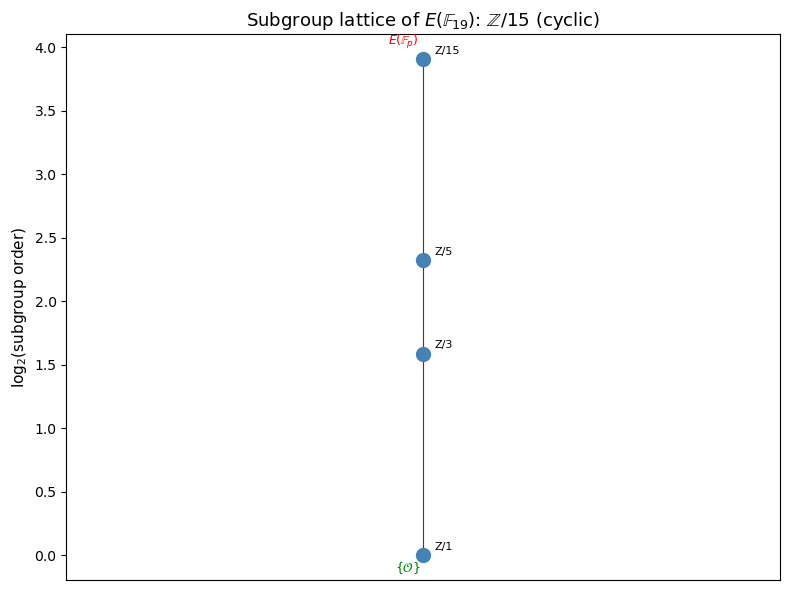
Comparing lattices
Notice that the lattice of \(\mathbb{Z}/8 \times \mathbb{Z}/2\) is wider than that of \(\mathbb{Z}/15\): at each level, there can be multiple subgroups of the same order. For the cyclic group \(\mathbb{Z}/15\), each divisor of 15 gives exactly one subgroup. This structural difference has consequences for cryptography: in a non-cyclic group, the discrete logarithm problem can potentially be decomposed into easier subproblems.
Invariant factors vs. subgroup lattice
The invariant-factor decomposition \(E(\mathbb{F}_p) \cong \mathbb{Z}/n_1 \times \mathbb{Z}/n_2\) tells us the isomorphism class (group type) of the point group, but it does not by itself describe the full subgroup lattice. Two groups can share the same invariant factors yet have subgroup lattices that look different when embedded in a larger context (for instance, considering the action of Frobenius or the rational structure over extension fields). The lattice diagrams above enumerate all abstract subgroups of the given abelian group; the actual subgroups realised over \(\mathbb{F}_p\) are always a subset of this abstract lattice.
32.14 The Collision Method for Point Counting#
When the group is cyclic, one can discover the group order via a collision method: choose a random point \(P\), compute successive doublings \(2^i P\), and look for a collision \(2^i P = 2^j P\) (with \(i \ne j\)). This implies \(\operatorname{ord}(P) \mid 2^i - 2^j\). From the factorisation of \(2^i - 2^j\), one can extract \(\operatorname{ord}(P)\) and check whether it falls in the Hasse interval \([p+1-2\sqrt{p},\, p+1+2\sqrt{p}]\).
import numpy as np
import math

def collision_method(E, P, max_steps=5000):
    """Find a collision 2^i P = 2^j P and return (i, j) with i > j."""
    seen = {}  # point -> step index
    Q = P
    for i in range(max_steps):
        key = Q  # points are tuples or 'O'
        if key in seen:
            return i, seen[key]
        seen[key] = i
        Q = ec_add(E, Q, Q)  # Q = 2*Q
    return None, None


def order_from_collision(E, P, i, j):
    """Given 2^i P = 2^j P, determine ord(P) by testing small prime factors of 2^i - 2^j."""
    # ord(P) divides 2^i - 2^j = 2^j (2^(i-j) - 1)
    diff_exp = i - j  # 2^j * (2^diff_exp - 1) divides the order relation

    # Instead of computing the huge number, we work with the exponent directly.
    # We know: (2^i - 2^j) * P = O, i.e., ord(P) | 2^j * (2^(i-j) - 1)
    # Try to narrow down the order using small factors.
    p = E['p']
    hasse_low = p + 1 - 2 * math.isqrt(p) - 1
    hasse_high = p + 1 + 2 * math.isqrt(p) + 1

    # Start with candidate = 2^j * (2^(i-j) - 1)
    # But this is huge. Instead, use small prime approach.
    # Compute candidate order by testing: for small primes q, check if (candidate/q)*P = O

    # First, find the order by computing (2^i - 2^j) mod possible orders in Hasse range
    for candidate_order in range(hasse_low, hasse_high + 1):
        if candidate_order <= 0:
            continue
        # Check if (2^i - 2^j) mod candidate_order == 0
        val = (pow(2, i, candidate_order) - pow(2, j, candidate_order)) % candidate_order
        if val == 0:
            # Verify: candidate_order * P == O
            if ec_mul(E, candidate_order, P) == 'O':
                # Verify it's the minimal such order (check divisors)
                order = candidate_order
                for (q, _) in trial_factor(candidate_order):
                    while order % q == 0 and ec_mul(E, order // q, P) == 'O':
                        order //= q
                return order
    return None


# Test: E(F_7927) with A=1, B=3
E7927 = ec_curve(1, 3, 7927)
P_col = (2643, 2059)
assert ec_on_curve(E7927, P_col), "Point not on curve!"

i, j = collision_method(E7927, P_col)
print(f"Collision found: 2^{i} P = 2^{j} P")

order = order_from_collision(E7927, P_col, i, j)
print(f"Order of P = {order}")

# Verify with naive count
N_verify = naive_count(1, 3, 7927)
print(f"Actual |E(F_7927)| = {N_verify}")
print(f"Order matches group size: {order == N_verify}")
print(f"Group is cyclic (generated by P): {order == N_verify}")
Collision found: 2^1580 P = 2^0 P
Order of P = 7925
Actual |E(F_7927)| = 7925
Order matches group size: True
Group is cyclic (generated by P): True
32.15 Sato-Tate Distribution: The Trace of Frobenius#
The Sato-Tate conjecture (now a theorem, proved by Taylor et al. in 2011 for non-CM curves over \(\mathbb{Q}\)) predicts that the normalised trace \(\theta = \arccos(a / (2\sqrt{p}))\) is distributed according to the density \(\frac{2}{\pi} \sin^2(\theta)\) on \([0, \pi]\).
Let us visualise this by computing the trace for many random curves.
Show code cell source
import numpy as np
import matplotlib.pyplot as plt
import math

p = 997
traces = []
rng = np.random.default_rng(0)

for _ in range(3000):
    A = int(rng.integers(1, p))
    B = int(rng.integers(1, p))
    disc = (4 * pow(A, 3, p) + 27 * pow(B, 2, p)) % p
    if disc == 0:
        continue
    N = naive_count(A, B, p)
    a = p + 1 - N
    # Normalise: theta = arccos(a / (2*sqrt(p)))
    normalised = a / (2 * math.sqrt(p))
    if -1 <= normalised <= 1:
        theta = math.acos(normalised)
        traces.append(theta)

traces = np.array(traces)

fig, ax = plt.subplots(figsize=(9, 5))
ax.hist(traces, bins=50, density=True, color='steelblue', edgecolor='white', alpha=0.8,
        label='Empirical (random curves)')

# Theoretical Sato-Tate density: (2/pi) * sin^2(theta)
theta_grid = np.linspace(0, np.pi, 300)
sato_tate = (2 / np.pi) * np.sin(theta_grid) ** 2
ax.plot(theta_grid, sato_tate, 'r-', linewidth=2.5, label='Sato-Tate density')

ax.set_xlabel(r'$\theta = \arccos(a\,/\,2\sqrt{p})$', fontsize=12)
ax.set_ylabel('Density', fontsize=12)
ax.set_title(f'Sato-Tate distribution for $p = {p}$', fontsize=14)
ax.legend(fontsize=11)
ax.set_xlim(0, np.pi)
plt.tight_layout()
plt.savefig('ch32_sato_tate.png', dpi=150, bbox_inches='tight')
plt.show()

print(f"Computed traces for {len(traces)} curves over F_{p}")
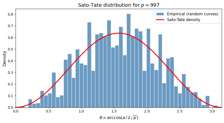
Computed traces for 2998 curves over F_997
32.16 Exercises#
Exercise 32.1: Point orders and cyclic detection
Consider the curve \(E: y^2 = x^3 + 11x + 3\) over \(\mathbb{F}_{193}\).
(a) Compute \(|E(\mathbb{F}_{193})|\) using the naive counting method.
(b) Find a point \(P\) on \(E\) and compute its order.
(c) Is \(E(\mathbb{F}_{193})\) cyclic? If so, find a generator. If not, find generators \(P_1, P_2\) for the two cyclic factors.
Hint
The group order should be close to \(p + 1 = 194\). For part (c), try computing the order of several random points. If the maximum order equals \(|E|\), the group is cyclic and that point is a generator.
Exercise 32.2: Non-cyclic group construction
Find an elliptic curve \(E\) over \(\mathbb{F}_p\) (for some small prime \(p < 100\)) such that \(E(\mathbb{F}_p)\) is not cyclic, i.e., \(E(\mathbb{F}_p) \cong \mathbb{Z}/n_1 \times \mathbb{Z}/n_2\) with \(n_2 > 1\).
(a) Find such a curve by systematic search.
(b) Verify that \(n_2 \mid n_1\) and \(n_2 \mid (p - 1)\).
(c) Explain why the condition \(n_2 \mid (p - 1)\) is necessary.
Hint
Try \(p = 11\) and test various \((A, B)\) pairs. The curve \(y^2 = x^3 + x + 2\) over \(\mathbb{F}_{11}\) is a known non-cyclic example with structure \(\mathbb{Z}/8 \times \mathbb{Z}/2\). Note \(n_2 = 2\) divides \(p - 1 = 10\).
Exercise 32.3: Collision method
Use the collision method to determine the order of the point group for each of these curves:
\((A, B) = (12, 5)\) over \(\mathbb{F}_{271}\)
\((A, B) = (199, 272)\) over \(\mathbb{F}_{1013}\)
(a) For each curve, find a point \(P\) and run the collision method.
(b) Verify that the order falls in the Hasse interval.
(c) If the order of \(P\) equals \(|E(\mathbb{F}_p)|\), the group is cyclic and \(P\) generates it. Verify this by checking that all multiples of \(P\) are distinct.
Hint
Start by finding a point: try \(x = 0, 1, 2, \ldots\) until \(x^3 + Ax + B\) is a quadratic
residue mod \(p\). Then apply collision_method and order_from_collision. The Hasse
interval is \([p + 1 - 2\lfloor\sqrt{p}\rfloor,\, p + 1 + 2\lfloor\sqrt{p}\rfloor]\).
Exercise 32.4: CRT and Schoof’s principle
Consider \(E: y^2 = x^3 + x + 1\) over \(\mathbb{F}_{1229}\).
(a) Compute \(|E(\mathbb{F}_{1229})|\) using the naive method.
(b) Find a \(3\)-torsion point (a point \(P\) with \(3P = \mathcal{O}\)) and determine \(a \bmod 3\) where \(a = p + 1 - |E|\).
(c) Find a \(47\)-torsion point and determine \(a \bmod 47\).
(d) Use the Chinese Remainder Theorem to reconstruct \(a\) from parts (b) and (c). Verify that \(p + 1 - a\) agrees with the naive count.
Hint
For \(p = 1229\), the Hasse bound gives \(|a| \le 2\sqrt{1229} \approx 70.1\). You need \(\prod \ell_i > 4\sqrt{p} \approx 140.2\), and indeed \(3 \times 47 = 141 > 140.2\). To find an \(\ell\)-torsion point, find any point \(Q\) and compute \((|E|/\ell) \cdot Q\); if \(\ell \mid |E|\), this gives an \(\ell\)-torsion point (possibly \(\mathcal{O}\), in which case try another \(Q\)).
Exercise 32.5: Subgroup lattice exploration
(a) Draw (by hand or using code) the subgroup lattice for \(\mathbb{Z}/12\). How many subgroups are there?
(b) Draw the subgroup lattice for \(\mathbb{Z}/6 \times \mathbb{Z}/2\). Compare it with the lattice for \(\mathbb{Z}/12\) – they have the same order (12) but different structures.
(c) For a group \(\mathbb{Z}/n_1 \times \mathbb{Z}/n_2\) with \(n_2 \mid n_1\), prove that the number of subgroups is at least the number of divisors of \(n_1 \cdot n_2\). When does equality hold?
Hint
For part (a), \(\mathbb{Z}/12\) has subgroups of orders \(1, 2, 3, 4, 6, 12\) (one for each divisor). For part (b), \(\mathbb{Z}/6 \times \mathbb{Z}/2\) has additional subgroups beyond those of \(\mathbb{Z}/12\): for example, it has three subgroups of order 2 (generated by \((3, 0)\), \((0, 1)\), and \((3, 1)\)). Equality in (c) holds when the group is cyclic (\(n_2 = 1\)).
32.17 Summary#
In this chapter we studied the algebraic structure of the point group \(E(\mathbb{F}_p)\):
Hasse’s theorem bounds \(|E(\mathbb{F}_p)|\) in the interval \([p + 1 - 2\sqrt{p},\, p + 1 + 2\sqrt{p}]\).
The structure theorem tells us \(E(\mathbb{F}_p) \cong \mathbb{Z}/n_1 \times \mathbb{Z}/n_2\) with \(n_2 \mid n_1\) and \(n_2 \mid (p - 1)\).
Naive counting is \(O(p)\) and only feasible for small primes.
Schoof’s algorithm computes \(|E(\mathbb{F}_p)|\) in polynomial time \(O(\log^8 p)\) by determining the trace of Frobenius modulo small primes and applying the CRT.
Most curves are cyclic: non-cyclic groups (where \(n_2 > 1\)) occur but are much rarer than cyclic groups for random curves over large fields, making cyclic groups overwhelmingly dominant in practice.
The Sato-Tate distribution describes how the trace of Frobenius distributes across random curves: the normalised angle follows a \(\frac{2}{\pi}\sin^2(\theta)\) density.
These results underpin the selection of elliptic curves for cryptographic applications. In the next chapter, we will use this theory to set up the Elliptic Curve Discrete Logarithm Problem (ECDLP) and study its hardness.
32.18 References#
Hasse, H. (1936). Zur Theorie der abstrakten elliptischen Funktionenkörper. Journal für die reine und angewandte Mathematik, 175, 193–208.
Schoof, R. (1985). Elliptic curves over finite fields and the computation of square roots mod \(p\). Mathematics of Computation, 44(170), 483–494.
Silverman, J.H. (2009). The Arithmetic of Elliptic Curves, 2nd edition. Springer GTM 106.
Washington, L.C. (2008). Elliptic Curves: Number Theory and Cryptography, 2nd edition. Chapman & Hall/CRC.
Taylor, R. (2008). Automorphy for some \(l\)-adic lifts of automorphic mod \(l\) Galois representations, II. Publ. Math. IHES, 108, 183–239. (Part of the Sato-Tate proof.)
Blake, I.F., Seroussi, G., Smart, N.P. (1999). Elliptic Curves in Cryptography. Cambridge University Press.