
Chapter 33: Elliptic Curve Cryptography in Practice (SageMath)#
Python Version Available
This notebook contains the SageMath implementation. A pure Python/NumPy version is available in Chapter 33: Elliptic Curve Cryptography in Practice.
33.1 Introduction#
Elliptic-curve cryptography (ECC) builds public-key protocols on top of the elliptic-curve discrete-logarithm problem (ECDLP):
Given points \(P\) and \(Q = [k]P\) on an elliptic curve \(E(\mathbb{F}_p)\), find the scalar \(k\).
The best generic algorithms for ECDLP run in \(O(\sqrt{n})\) time, which means a 256-bit elliptic-curve group offers roughly the same security as a 3072-bit RSA modulus. This chapter implements the two most widely deployed ECC protocols — ECDH (key exchange) and ECDSA (digital signatures) — and then examines attacks that exploit weak curve parameters.
All arithmetic is performed over small prime fields so that every step is
transparent. We use SageMath’s built-in EllipticCurve, GF, and
factor facilities for curve construction, point arithmetic, and group
order analysis.
Prerequisites
Chapter 31 (finite-field arithmetic on curves) and Chapter 32 (group structure and the ECDLP) are assumed.
33.2 Warm-up: Curves over Small Fields#
Before diving into cryptographic protocols, let us review how SageMath handles elliptic curves over finite fields.
We initialise the curve \(y^2 = x^3 + x + 2\) over \(\mathbb{F}_5\).
When \(x\) and \(y\) belong to the ring \(\mathbb{Z}/5=\{0,1,2,3,4\}\) it is easy to find all solutions to the congruence \(y^2\equiv x^3+x+2(\textrm{mod }5)\).
We perform both addition and multiplication in \(\mathbb{Z}/5\) in the usual \(\textrm{mod }5\) way. These two operations constitute a structure of a field on \(\mathbb{Z}/5\). We denote this structure as \(\mathbb{F}_{5}\).
For example: \(2+3=0\) in \(\mathbb{F}_{5}\). We can write both the addition and multiplication table:
F5=GF(5)
#addition table
add=[[0]+[F5(i) for i in range(0,5)]]+[[F5(i)]+[F5(i)+F5(j) for j in range(0,5)] for i in range(0,5)];
pretty_print(matrix(add))
#multiplication table
mul=[[0]+[F5(i) for i in range(1,5)]]+[[F5(i)]+[F5(i)*F5(j) for j in range(1,5)] for i in range(1,5)];
pretty_print(matrix(mul))
E=EllipticCurve([GF(5)(1),2]);
We generate all points on \(E\) over the finite field \(\mathbb{F}_5\).
Apart from the points of the form \((x,y)\) we have one additional point ‘at infinity’ which is the neutral point of the group law on \(E\).
E.rational_points() #(x:y:1) - projective coordinates of the point (x,y);
                    #(0:1:0) - point at infinity
[(0 : 1 : 0), (1 : 2 : 1), (1 : 3 : 1), (4 : 0 : 1)]
The group under consideration is formed from the set \(E(\mathbb{F}_{5})\) which consists of \(3\) points \((1,2), (1,3)\) and \((4,0)\)
and one more point at ‘infinity’. \((0:1:0)\) (the notation is different because this point has ‘‘zero denominator’’, which makes the form \((x,y)\) impossible to write.
P=E([1,2]) #we pick one of these points
We add the point \(P\) several times to itself. It will turn out that the points listed above are multiples of \(P\). That means that the group \(E(\mathbb{F}_{5})\) is cyclic and generated by \(P\)!
print(P)
print(2*P)
print(3*P)
print(4*P)
(1 : 2 : 1)
(4 : 0 : 1)
(1 : 3 : 1)
(0 : 1 : 0)
Algebraic group law on \(E\) is expressed by a complicated formula which we reveal below.
Fx.<x>=FunctionField(GF(5))
RY.<Y>=Fx[]
Fy.<y>=Fx.extension(x^3+x+3-Y^2)
Fw.<w>=FunctionField(Fy)
RZ.<Z>=Fw[]
Fz.<z>=Fw.extension(w^3+w+3-Z^2)
EF=EllipticCurve([Fz(1),3])
P1=EF([x,y])
P2=EF([w,z])

(P1+P2)[0]==(1 + w + x + w^2*x + w*x^2 + 3*y*z)/(w^2 + 3*w*x + x^2)
(P1+P2)[1]==(2*y + 3*w*y + w^3*y + x*y + 3*w^2*x*y + 3*z + 4*w*z + 2*x*z + 2*w*x^2*z + 4*x^3*z)/(w^3 + 2*w^2*x + 3*w*x^2 + 4*x^3)
True
pretty_print(P1+P2)
Addition of points on \(E\) is complicated algebraically but intuitive geometrically. At the same time these computations can be performed fast on the computer.
pretty_print(2*P1)
In principle, the curve above could be used for cryptographic purposes but the group under consideration has only \(4\) elements which is obviously not safe enough for any reasonable coding.
What we need to change is first of all the field of definition of our curve.
In practice, we need point orders of at least 256 bits (approximately \(10^{77}\)) to achieve adequate security. Standard curves like NIST P-256 use a prime-order group of that size, providing roughly 128-bit security against generic attacks such as Pollard’s rho.
33.3 Encoding Messages on Curves (Koblitz Method)#
Definition: Koblitz encoding
We encode our message \(m\) as a point on the curve. The first coordinate is going to be \(\kappa\cdot m+j\), where our message should be \(m<p/\kappa\) and \(1\leq j\leq \kappa\). This guarantees we will find a suitable point in the randomised procedure (with chance of success \(1-1/2^\kappa\)). Coordinate \(y\) is chosen in such a way that \(y^2=x^3+ax+b\), where \(a,b\) are fixed, and \(x=\kappa\cdot m+j\) for a fixed \(j\).
#letter encoding (not reasonable, why?)
def EncodePoint(E,char,kappa=100):
    p=E.base_field().characteristic() #field characteristic
    m=ord(char) #ASCII code
    assert m <= p*1.0/kappa
    pol=E.defining_polynomial()
    for i in range(0,kappa):
        val=-pol([kappa*m+i,0,1])
        if val.is_square():
            sq=sqrt(val)
            P=E([kappa*m+i,sq,1])
            break;

    return P
EE=EllipticCurve([GF(160174168162444816244821958911111)(1),3])
EncodePoint(EE,"m")
(10901 : 42332909399061611549525231919913 : 1)
RealField(20)(log(EE.order(),10)) #EE.order() ~= 10^32, is a large number!
32.205
#unfortunately the cyclic subgroups here are of rather small order which means we
#should choose a better curve
EE.order().factor()
2^3 * 5 * 41 * 59 * 269 * 1232450832397 * 4993151403869
Decoding procedure is very simple. We compute the floor of the expression \(x/\kappa\), where \(x\) is the first coordinate of a point.
def DecodePoint(P,kappa=100):
    x=int(P[0])
    return chr(int(x/kappa))
Exemplary coding and decoding of a point (points on the curve are not displayed)
alphabet=[ "a", "b", "c", "d", "e", "f", "g", "h", "i", "j", "k", "l", "m", "n", "o",
"p", "q", "r", "s", "t", "u", "v", "w", "x", "y", "z" ];
EE=EllipticCurve([GF(160174168162444816244821958911111)(1),3]);
print([DecodePoint(EncodePoint(EE,x)) for x in alphabet])==alphabet
['a', 'b', 'c', 'd', 'e', 'f', 'g', 'h', 'i', 'j', 'k', 'l', 'm', 'n', 'o', 'p', 'q', 'r', 's', 't', 'u', 'v', 'w', 'x', 'y', 'z']
False
Point orders and group order
The orders of points are not always equal to the order of the group, which makes our cryptosystem weaker. It is reasonable to choose our group in such a way that there are just a few prime factors in the group order.
pp=[(EncodePoint(EE,x)) for x in alphabet]
[x.order()==EE.order() for x in pp]
[False,
 True,
 False,
 True,
 False,
 False,
 False,
 False,
 True,
 True,
 False,
 False,
 False,
 True,
 False,
 True,
 False,
 True,
 False,
 False,
 True,
 True,
 False,
 False,
 True,
 True]
33.4 ECDH — Elliptic-Curve Diffie–Hellman#
The Elliptic-Curve Diffie–Hellman protocol is the curve analogue of classical DH key exchange. Two parties, Alice and Bob, agree on public parameters \((E, P, n)\) where \(P\) is a base point of order \(n\).
Step |
Alice |
Bob |
|---|---|---|
1 |
Choose secret \(a\); publish \(A = [a]P\) |
Choose secret \(b\); publish \(B = [b]P\) |
2 |
Compute \(S = [a]B = [ab]P\) |
Compute \(S = [b]A = [ab]P\) |
Both parties arrive at the same shared secret \(S = [ab]P\) without ever transmitting \(a\) or \(b\). Security reduces to the Computational Diffie–Hellman (CDH) problem on the curve.
In SageMath, we use EllipticCurve(GF(p), [a, b]) to define the curve
and native point multiplication k * P for scalar multiplication.
# -- ECDH on y^2 = x^3 + 2x + 15 over F_97 --
# Using a curve with prime group order (107) for reliable protocols
p = 97; a_coeff = 2; b_coeff = 15
E = EllipticCurve(GF(p), [a_coeff, b_coeff])
G = E([1, 42])  # generator
n = G.order()
print(f'Curve: y^2 = x^3 + {a_coeff}x + {b_coeff}  (mod {p})')
print(f'Generator G = {G},  order = {n}')
Curve: y^2 = x^3 + 2x + 15  (mod 97)
Generator G = (1 : 42 : 1),  order = 107
# Alice
set_random_seed(42)
a_priv = randint(1, n - 1)
A_pub = a_priv * G
print(f'Alice: private = {a_priv},  public A = {A_pub}')

# Bob
set_random_seed(99)
b_priv = randint(1, n - 1)
B_pub = b_priv * G
print(f'Bob:   private = {b_priv},  public B = {B_pub}')

# Shared secret
S_alice = a_priv * B_pub
S_bob   = b_priv * A_pub
print(f'\nAlice computes S = {S_alice}')
print(f'Bob   computes S = {S_bob}')
print(f'Shared secrets match: {S_alice == S_bob}')
Alice: private = 47,  public A = (23 : 43 : 1)
Bob:   private = 8,  public B = (59 : 58 : 1)

Alice computes S = (63 : 5 : 1)
Bob   computes S = (63 : 5 : 1)
Shared secrets match: True
Why ECDH beats classical DH
For 128-bit security, classical DH requires a 3072-bit prime, while ECDH needs only a 256-bit curve. Key generation and shared-secret computation are both faster and produce shorter keys.
33.5 Elliptic ElGamal Cryptosystem#
Public key: selected elliptic curve \(E:y^2=x^3+ax+b\), fixed point \(P\) and point \(B\) which is an \(s\)-multiple of \(P\).
Private key: integer \(s\).
Alice sends a message \(M\) to Bob and encodes it as a sequence of symbols. For simplicity we assume that \(\tilde{m}\) represents a single letter (why this is bad, explain). Symbol \(\tilde{m}\) is encoded as a point on the elliptic curve \(E\).
def EncodeElGamal(char,public_key):
    E,P,B=public_key
    m=EncodePoint(E,char)
    k=randint(1,10^10)
    M1=k*P
    M2=m+k*B
    return (M1,M2)
Bob generates his private key \(s\) and a public key for Alice.
s=2020; #this is secret (better to choose randomly)
E=EllipticCurve([GF(160174168162444816244821958911111)(1),3])
P=E.gens()[0] #this is one of the large order generators
BobPublicKey=(E,P,s*P) #generating a public key is fast
%timeit BobPublicKey=(E,P,s*P)
26.2 μs ± 3 μs per loop (mean ± std. dev. of 7 runs, 10,000 loops each)
Now, we only need to write a decryption procedure of the ElGamal protocol.
def DecodeElGamal(encoded_message,secret):
    M1,M2=encoded_message
    m=M2-secret*M1
    return DecodePoint(m)
Testing ElGamal#
encrypted_char=EncodeElGamal("a",BobPublicKey)
print("Cryptogram:")
print(encrypted_char)
Cryptogram:
((127186194458596706675934158377818 : 109254454223149324656428247715959 : 1), (10451303170838791351088794210754 : 140417541533607506552449256150622 : 1))
decoded_char=DecodeElGamal(encrypted_char,s);
print("Plain text")
print(decoded_char)
Plain text
a
Sending a longer message#
#secret message
message="Santa Claus is coming to town!";
Preparing a message
#secret computation on Alice's computer
cipher=[];
for i in [0..len(message)-1]:
    cipher.append(EncodeElGamal(message[i],BobPublicKey))
Our ciphertext looks complicated enough
print(cipher)
[((88754055202807240826457994739731 : 123651553228241701995443802024215 : 1), (136643374313131550609056365206222 : 119413187727415398654155098515087 : 1)), ((140993361985861783409354921874639 : 14702260542316621709669252396216 : 1), (155361326792522889533542570728239 : 32382069188072450595626775947123 : 1)), ((52476224141289507724459654828498 : 17844455751672962332257351331426 : 1), (63005878806415406297240246640764 : 117858124866278158184766881561803 : 1)), ((129577116265235893751090885270280 : 97536352840093858921460292015056 : 1), (95117270000534415109653918584622 : 155257028476570156997896979393703 : 1)), ((158947791206389038809435507896382 : 11746697135517623743763844757758 : 1), (45834000603422942477700714313401 : 94715130810474753103353030984240 : 1)), ((137070153584347304673414219939940 : 5797878320722646805563903722699 : 1), (142628152071757306068909781127407 : 131705212147088495181048604226298 : 1)), ((21850993980640461816324509386686 : 114825038463875915284275964314084 : 1), (144077138129673280003811971911432 : 28207321186809835074387946744073 : 1)), ((41960003274603396490598777091940 : 152062272964116820160000967052851 : 1), (85906925531729802515610576035847 : 133187398806311741981824971150942 : 1)), ((96526924613441583459322085291900 : 89826765797264158173267305703036 : 1), (81926748498873734707525567755231 : 148405763296515465741236234414030 : 1)), ((12710203290273322564673726719226 : 87919045801808781007440321199184 : 1), (4768549249993895229557578096857 : 72094664247182421858394264013384 : 1)), ((21295333190962984581530576117684 : 30104826090679993481673718217923 : 1), (86885975993146044970492010907566 : 55919658342948337511034969701080 : 1)), ((42643339380197052380151264437126 : 55518965963908433288187424495266 : 1), (70570277018279879434400076986009 : 67741397447817482404461144637755 : 1)), ((147249731035274602616568891015517 : 8989803236669216983007342817410 : 1), (6344607625415267793480701992292 : 114671111290267925160200788451748 : 1)), ((45805226983549675639012969293548 : 87952290255878483112299895105321 : 1), (75616063651411381838099144898161 : 57152574093877284665305341193889 : 1)), ((102365585431936089819956192062887 : 134634393666385056508697691131766 : 1), (137587369138697333520924123395448 : 56744666253689762775251352800590 : 1)), ((14617748014855090334315243781804 : 73279051193479671030270245572090 : 1), (58945772412512274420537565529337 : 117237619756526220483493678035750 : 1)), ((85960804419892863932325710362449 : 103209354814049169729300418341834 : 1), (46553586620026674466748464990476 : 34285086813333299127757651226690 : 1)), ((63070740069015663648742844187714 : 12725591418381312885599101634696 : 1), (109609961889470367599242439690244 : 81352731161026864654650765905368 : 1)), ((91738795308286709870950214746095 : 21730494336325458093701840825755 : 1), (132920975546960497564402452590162 : 25209666640129089650645302652584 : 1)), ((146810824100633178709502244435183 : 41586901429481089242902058516487 : 1), (6881203165024452198554546907234 : 5752959212169546838614115599673 : 1)), ((118741781589420484637197063293760 : 7035876436516412571030212584205 : 1), (125076685127018061457334460584453 : 138223467542461774103507537879010 : 1)), ((16412716239932765354900825607663 : 157087322405527438934631006633033 : 1), (81973251018638587490888990861482 : 67294248766559726742520768330941 : 1)), ((138596176093079520434493917190647 : 32947512499067423925294412046148 : 1), (155923140055278715673094925354706 : 5284531364119482823220290670327 : 1)), ((144984809243183486370684047733026 : 117740585177105863071135854915524 : 1), (107945502495495363003069836085116 : 40155120896184500149595632407778 : 1)), ((41970701080142165034338335965019 : 51602097850805429308983024147615 : 1), (115395883512511211538346181279898 : 149389082058074436295756394900123 : 1)), ((38357970214545961191297731895509 : 38242644932958734885322553858492 : 1), (123369365786044115447402218919409 : 127250827101205912836949395627246 : 1)), ((72591751492763579137200134845262 : 124303270184025695518106737062770 : 1), (5385286883746158806063729479714 : 135338359353448374814725314530107 : 1)), ((67998121312671716208478508691956 : 62335618706582296863409735697141 : 1), (109915762039799404262229418342255 : 77889689447311005472107722695607 : 1)), ((42827927108190862828959325044127 : 64774599826005410527591874887659 : 1), (70257785385649808465575872167806 : 14278791845497006023524013373122 : 1)), ((140434381546738912216609963356396 : 128252134398132165671836824517547 : 1), (81828977806956334634237456182123 : 19643191702668979572028703582317 : 1))]
We send our cipher through a public channel. If no one guessed our secret key \(s\), it will be very hard to get your hands on the message (DLP type problem).
Deciphering happens on Bob’s computer with the help of the secret key \(s\).
#Bob's deciphering procedure
plain_text=[DecodeElGamal(char,s) for char in cipher]
print(''.join(plain_text))
Santa Claus is coming to town!
33.6 ECDSA — Elliptic-Curve Digital Signature Algorithm#
ECDSA adapts the classical DSA scheme to elliptic curves. Public parameters are the same as for ECDH: \((E, P, n)\) with \(P\) of prime order \(n\).
Key generation. Choose private key \(d \in \{1,\dots,n-1\}\); publish \(Q = [d]P\).
Signing a message \(m\):
Compute hash \(e = H(m)\).
Pick random \(k \in \{1,\dots,n-1\}\).
Compute \(R = [k]P\); set \(r = x_R \bmod n\). If \(r = 0\), go to 2.
Compute \(s = k^{-1}(e + d \cdot r) \bmod n\). If \(s = 0\), go to 2.
Signature is \((r, s)\).
Verification of \((r, s)\) on message \(m\):
Compute \(e = H(m)\).
Compute \(w = s^{-1} \bmod n\).
Compute \(u_1 = e \cdot w \bmod n\), \(u_2 = r \cdot w \bmod n\).
Compute \(R' = [u_1]P + [u_2]Q\).
Accept iff \(x_{R'} \equiv r \pmod{n}\).
# -- ECDSA (toy implementation) in SageMath --
import hashlib

def ecdsa_hash(m, n):
    """Hash using SHA-256 reduced modulo n (toy but collision-resistant)."""
    if isinstance(m, str):
        m = m.encode('utf-8')
    elif isinstance(m, int):
        m = str(m).encode('utf-8')
    h = hashlib.sha256(m).hexdigest()
    return ZZ('0x' + h) % n

def ecdsa_sign(m, d, G, n):
    """Sign message m with private key d. Return (r, s)."""
    e = ecdsa_hash(m, n)
    while True:
        k = randint(1, n - 1)
        R = k * G
        if R.is_zero():
            continue
        r = ZZ(R.xy()[0]) % n
        if r == 0:
            continue
        k_inv = inverse_mod(k, n)
        s = (k_inv * (e + d * r)) % n
        if s == 0:
            continue
        return (r, s)

def ecdsa_verify(m, signature, Q, G, n):
    """Verify signature (r, s) on message m with public key Q."""
    r, s = signature
    if not (1 <= r < n and 1 <= s < n):
        return False
    e = ecdsa_hash(m, n)
    w  = inverse_mod(s, n)
    u1 = (e * w) % n
    u2 = (r * w) % n
    R_prime = u1 * G + u2 * Q
    if R_prime.is_zero():
        return False
    return ZZ(R_prime.xy()[0]) % n == r

print('ECDSA functions defined.')
ECDSA functions defined.
# -- Demo: ECDSA on y^2 = x^3 + 2x + 15 over F_97 --
# Using a curve with prime group order (107) for reliable ECDSA
p = 97; a_coeff = 2; b_coeff = 15
E = EllipticCurve(GF(p), [a_coeff, b_coeff])
G = E([1, 42])
n = G.order()

# Key generation
set_random_seed(2024)
d = randint(1, n - 1)
Q = d * G
print(f'Curve: y^2 = x^3 + {a_coeff}x + {b_coeff} (mod {p}), order = {n}')
print(f'Private key d = {d}')
print(f'Public key  Q = {Q}')

# Sign
msg = 'hello'
set_random_seed(7777)
sig = ecdsa_sign(msg, d, G, n)
print(f'\nMessage:   "{msg}"')
print(f'Signature: (r={sig[0]}, s={sig[1]})')

# Verify
ok  = ecdsa_verify(msg, sig, Q, G, n)
bad = ecdsa_verify('world', sig, Q, G, n)
print(f'\nVerify "{msg}":  {ok}')
print(f'Verify "world": {bad}')
Curve: y^2 = x^3 + 2x + 15 (mod 97), order = 107
Private key d = 33
Public key  Q = (58 : 51 : 1)

Message:   "hello"
Signature: (r=87, s=91)

Verify "hello":  True
Verify "world": False
Nonce reuse is catastrophic
If the same nonce \(k\) is used for two different messages \(m_1, m_2\), then \(r_1 = r_2\) and an attacker can recover the private key:
This is exactly the attack that compromised the PlayStation 3 ECDSA implementation in 2010.
# -- Nonce-reuse attack demonstration --
# Using a curve with prime group order for reliable ECDSA
p = 97; a_coeff = 2; b_coeff = 15
E = EllipticCurve(GF(p), [a_coeff, b_coeff])
G = E([1, 42])
n = G.order()

set_random_seed(1234)
d_secret = randint(1, n - 1)
Q_pub = d_secret * G

# Alice signs two messages with THE SAME nonce (bad!)
m1, m2 = 'msg_one', 'msg_two'
set_random_seed(5555)
sig1 = ecdsa_sign(m1, d_secret, G, n)
set_random_seed(5555)  # same seed => same nonce k
sig2 = ecdsa_sign(m2, d_secret, G, n)

r1, s1 = sig1
r2, s2 = sig2
e1 = ecdsa_hash(m1, n)
e2 = ecdsa_hash(m2, n)

print(f'sig1: r={r1}, s={s1}   (r values match: r1==r2 is {r1==r2})')
print(f'sig2: r={r2}, s={s2}')

# Recover private key
numerator   = (s2 * e1 - s1 * e2) % n
denominator = (s1 * r2 - s2 * r1) % n
d_recovered = (numerator * inverse_mod(denominator, n)) % n

print(f'\nTrue private key:      {d_secret}')
print(f'Recovered private key: {d_recovered}')
print(f'Attack succeeded: {d_secret == d_recovered}')
sig1: r=45, s=57   (r values match: r1==r2 is True)
sig2: r=45, s=1

True private key:      58
Recovered private key: 58
Attack succeeded: True
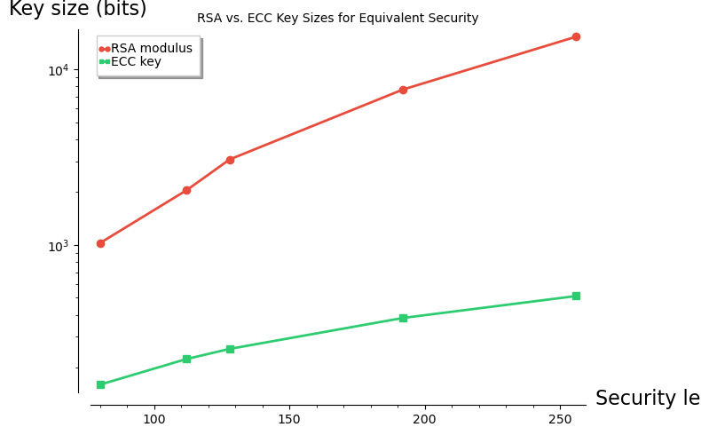
33.7 Security Comparison: RSA vs. ECC Key Sizes#
The following table (based on NIST SP 800-57 recommendations) compares the key lengths needed for equivalent security levels.
# NIST SP 800-57 recommended key sizes
security_bits = [80, 112, 128, 192, 256]
rsa_bits      = [1024, 2048, 3072, 7680, 15360]
ecc_bits      = [160, 224, 256, 384, 512]

# SageMath bar chart
from sage.plot.bar_chart import BarChart

G_rsa = bar_chart(rsa_bits, color='#e74c3c', width=0.4)
G_ecc = bar_chart(ecc_bits, color='#2ecc71', width=0.4)

# Use a text table for clarity (SageMath bar_chart is limited)
header = f'{"Security (bits)":>16s}  {"RSA modulus":>12s}  {"ECC key":>10s}  {"Ratio":>7s}'
print(header)
print('-' * len(header))
for sb, rb, eb in zip(security_bits, rsa_bits, ecc_bits):
    print(f'{int(sb):>16d}  {int(rb):>12d}  {int(eb):>10d}  {float(rb/eb):>7.1f}x')

print(f'\nAt 256-bit security, RSA needs 15360 bits vs. ECC\'s 512 bits.')
 Security (bits)   RSA modulus     ECC key    Ratio
---------------------------------------------------
              80          1024         160      6.4x
             112          2048         224      9.1x
             128          3072         256     12.0x
             192          7680         384     20.0x
             256         15360         512     30.0x

At 256-bit security, RSA needs 15360 bits vs. ECC's 512 bits.
# SageMath visualisation of RSA vs ECC key sizes
rsa_plot = list_plot(
    list(zip(security_bits, rsa_bits)),
    plotjoined=True, color='#e74c3c', marker='o',
    legend_label='RSA modulus', thickness=2
)
ecc_plot = list_plot(
    list(zip(security_bits, ecc_bits)),
    plotjoined=True, color='#2ecc71', marker='s',
    legend_label='ECC key', thickness=2
)
combined = rsa_plot + ecc_plot
combined.axes_labels(['Security level (bits)', 'Key size (bits)'])
show(combined, title='RSA vs. ECC Key Sizes for Equivalent Security',
     figsize=(8, 5), scale='semilogy')
33.8 Attacking the ECDLP#
The security of ECDH and ECDSA rests on the hardness of the ECDLP. We now study two classical attacks:
Pohlig–Hellman decomposition (exploits smooth group order).
Pollard’s rho algorithm (generic \(O(\sqrt{n})\) attack).
A third, more theoretical attack — the MOV attack — uses pairings to transfer the ECDLP into a finite-field DLP, where sub-exponential algorithms (index calculus) apply.
33.8.1 Baby-Step Giant-Step for ECDLP#
The BSGS algorithm solves the ECDLP in \(O(\sqrt{n})\) time and space.
In SageMath, we can use the built-in discrete_log function, but
let us also implement BSGS directly using SageMath point arithmetic.
def bsgs_ec(G, Q, n):
    """Baby-step giant-step for ECDLP: find k s.t. k*G = Q.

    Parameters
    ----------
    G : base point (SageMath elliptic curve point)
    Q : target point = k*G
    n : order of G
    """
    m = isqrt(n) + 1
    # Baby steps: table[j*G] = j for j = 0..m-1
    table = {}
    R = G.curve()(0)  # point at infinity
    for j in range(m):
        table[R] = j
        R = R + G

    # Giant step factor: -m*G
    factor = -(m * G)

    # Giant steps
    gamma = Q
    for i in range(m):
        if gamma in table:
            k = (i * m + table[gamma]) % n
            return k
        gamma = gamma + factor

    raise ValueError('BSGS failed')

# Quick test
p = 97; a_c = 2; b_c = 15
E = EllipticCurve(GF(p), [a_c, b_c])
G = E([1, 42])
n = G.order()
k_test = 17
Q_test = k_test * G
k_found = bsgs_ec(G, Q_test, n)
print(f'BSGS: k*G = Q  =>  k = {k_found}  (expected {k_test})')
BSGS: k*G = Q => k = 17 (expected 17)
# Compare with SageMath built-in discrete_log
k_builtin = discrete_log(Q_test, G, n, operation='+')
print(f'SageMath discrete_log: k = {k_builtin}')
print(f'Match: {k_builtin == k_found}')
SageMath discrete_log: k = 17
Match: True
33.8.2 Pohlig–Hellman on Elliptic Curves#
If the group order \(n = |\langle P \rangle|\) factors as \(n = \prod p_i^{e_i}\) with small prime powers, then we can:
For each prime power \(p_i^{e_i}\), project the ECDLP into a subgroup of order \(p_i^{e_i}\) and solve a much smaller DLP.
Combine the results via the Chinese Remainder Theorem.
The total cost is \(O\bigl(\sum e_i (\log n + \sqrt{p_i})\bigr)\), which is devastating when all \(p_i\) are small (“smooth” order).
def pohlig_hellman_ec(G, Q, n):
    """Pohlig-Hellman decomposition for ECDLP: find k s.t. k*G = Q.

    Uses SageMath's factor() and CRT.
    Works well when the group order n has only small prime factors.
    """
    fac = factor(n)
    residues = []
    moduli   = []

    for pi, ei in fac:
        pe = pi^ei
        # Project into subgroup of order pi^ei
        exp = n // pe
        Gi = exp * G   # order pi^ei
        Qi = exp * Q

        # Solve ECDLP in small subgroup using BSGS
        ki = bsgs_ec(Gi, Qi, pe)
        residues.append(ki)
        moduli.append(pe)

    return crt(residues, moduli)

print('pohlig_hellman_ec defined.')
pohlig_hellman_ec defined.
# -- Pohlig-Hellman attack on a curve with smooth order --
# Curve: y^2 = x^3 + x + 6 over F_101
p = 101; a_c = 1; b_c = 6
E = EllipticCurve(GF(p), [a_c, b_c])
N = E.order()
print(f'Curve: y^2 = x^3 + x + 6 (mod {p})')
print(f'#E(F_{p}) = {N}')
print(f'Factorisation of {N}: {factor(N)}')

# Find a generator
pts = E.rational_points()
G = pts[1]  # first non-trivial point
n = G.order()
print(f'\nGenerator G = {G},  ord(G) = {n}')
print(f'Factorisation of order: {factor(n)}')

# Secret scalar
k_secret = 73
Q = k_secret * G
print(f'\nSecret k = {k_secret},  Q = k*G = {Q}')

# Attack
k_found = pohlig_hellman_ec(G, Q, n)
print(f'Pohlig-Hellman recovered k = {k_found}')
print(f'Verification: {k_found}*G = {k_found * G}  ==  Q = {Q}')
print(f'Success: {k_found * G == Q}')
Curve: y^2 = x^3 + x + 6 (mod 101)
#E(F_101) = 112
Factorisation of 112: 2^4 * 7

Generator G = (0 : 39 : 1),  ord(G) = 112
Factorisation of order: 2^4 * 7

Secret k = 73,  Q = k*G = (46 : 78 : 1)
Pohlig-Hellman recovered k = 73
Verification: 73*G = (46 : 78 : 1)  ==  Q = (46 : 78 : 1)
Success: True
Smooth-order curves are insecure
The Pohlig–Hellman attack shows why NIST and other standards require that the curve group order contain a large prime factor. In practice, \(n\) itself is usually chosen to be prime.
33.8.3 Pollard’s Rho for ECDLP#
Pollard’s rho is a generic \(O(\sqrt{n})\) algorithm that needs only \(O(1)\) memory. The idea is to define a pseudo-random walk on the group \(\langle P \rangle\) and detect a collision.
We partition the group into three subsets \(S_0, S_1, S_2\) (e.g., by \(x \bmod 3\)) and define the iteration:
Each \(R_i = [a_i]P + [b_i]Q\) with known \(a_i, b_i\). When a collision \(R_i = R_j\) occurs, we have \(a_i - a_j \equiv k(b_j - b_i) \pmod{n}\), which reveals \(k\).
def pollard_rho_ec(G, Q, n):
    """Pollard rho for ECDLP: find k s.t. k*G = Q.
    Uses SageMath point arithmetic and Floyd's cycle detection.
    """
    E = G.curve()
    O = E(0)  # point at infinity

    def step(R, aR, bR):
        if R == O:
            x_mod = 0
        else:
            x_mod = ZZ(R.xy()[0]) % 3
        if x_mod == 0:
            R  = R + Q
            bR = (bR + 1) % n
        elif x_mod == 1:
            R  = R + R
            aR = (2 * aR) % n
            bR = (2 * bR) % n
        else:
            R  = R + G
            aR = (aR + 1) % n
        return R, aR, bR

    # Floyd's cycle detection
    # Tortoise
    T, aT, bT = G, 1, 0
    # Hare
    H, aH, bH = G, 1, 0

    for _ in range(3 * n):
        T, aT, bT = step(T, aT, bT)
        H, aH, bH = step(*step(H, aH, bH))

        if T == H:
            db = (bT - bH) % n
            da = (aH - aT) % n
            if db == 0:
                continue
            g = gcd(db, n)
            if g == 1:
                return (da * inverse_mod(db, n)) % n
            else:
                base = (da // g * inverse_mod(db // g, n // g)) % (n // g)
                for j in range(g):
                    candidate = (base + j * (n // g)) % n
                    if candidate * G == Q:
                        return candidate
            # Reset if no solution found
            T, aT, bT = G, 1, 0
            H, aH, bH = G, 1, 0

    raise ValueError('Pollard rho did not converge')

print('pollard_rho_ec defined.')
pollard_rho_ec defined.
# -- Demo: Pollard rho on a small curve --
p = 97; a_c = 2; b_c = 15
E = EllipticCurve(GF(p), [a_c, b_c])
G = E([1, 42])
n = G.order()

k_secret = 41
Q = k_secret * G

print(f'Curve: y^2 = x^3 + {a_c}x + {b_c} (mod {p})')
print(f'G = {G}, ord(G) = {n}')
print(f'Q = {Q}  (secret k = {k_secret})')

k_found = pollard_rho_ec(G, Q, n)
print(f'\nPollard rho found k = {k_found}')
print(f'Verification: {k_found}*G = {k_found * G}')
print(f'Match: {k_found * G == Q}')
Curve: y^2 = x^3 + 2x + 15 (mod 97)
G = (1 : 42 : 1), ord(G) = 107
Q = (29 : 55 : 1)  (secret k = 41)

Pollard rho found k = 41
Verification: 41*G = (29 : 55 : 1)
Match: True
# -- Measure Pollard-rho runtime vs. group order --
import time

test_curves = [
    # (a, b, p, Gx, Gy) -- small curves with verified generators
    (2, 3,  23,   1,  11),
    (2, 3,  43,   1,   7),
    (2, 3,  67,   3,   6),
    (2, 15, 97,   1,  42),
    (1, 6,  101,  0,  39),
    (2, 3,  131,  5,  20),
    (2, 3,  157,  4,  46),
    (3, 7,  199,  0,  87),
]

orders = []
times  = []

for (a_c, b_c, pp, gx, gy) in test_curves:
    Ei = EllipticCurve(GF(pp), [a_c, b_c])
    GG = Ei([gx, gy])
    nn = GG.order()
    if nn < 5:
        continue
    k_test = nn // 3 + 1
    Qt = k_test * GG
    t0 = time.perf_counter()
    kk = pollard_rho_ec(GG, Qt, nn)
    elapsed = time.perf_counter() - t0
    assert kk * GG == Qt
    orders.append(nn)
    times.append(elapsed)

# SageMath scatter plot
sqrt_orders = [float(sqrt(o)) for o in orders]
times_ms = [t * 1000 for t in times]
pts_data = list(zip(sqrt_orders, times_ms))

P_plot = point2d(pts_data, color='#e74c3c', size=60, zorder=5)
P_plot.axes_labels([r'$\sqrt{n}$  (group order)', 'Time (ms)'])
show(P_plot, title=r'Pollard Rho: Runtime vs. $\sqrt{n}$',
     figsize=(7, 4.5), gridlines=True)
print(f'Timings collected for {len(orders)} curves.')

Timings collected for 8 curves.
33.9 The MOV Attack (Conceptual)#
The Menezes–Okamoto–Vanstone (MOV) attack (1993) reduces the ECDLP to the ordinary discrete-logarithm problem in a finite field \(\mathbb{F}_{p^k}^*\) using the Weil pairing (or Tate pairing).
Key idea. Let \(P\) have order \(n\) on \(E(\mathbb{F}_p)\) and let \(Q = [d]P\). There exists a bilinear, non-degenerate map
(the Weil pairing), where \(k\) is the embedding degree — the smallest integer such that \(n \mid p^k - 1\).
Applying the pairing:
for a suitable second point \(R\). Now we need to solve \(\alpha^d = \beta\) in \(\mathbb{F}_{p^k}^*\) — a finite-field DLP vulnerable to index-calculus methods.
When is the MOV attack practical?
The attack is efficient only when the embedding degree \(k\) is small. For supersingular curves over \(\mathbb{F}_p\) with \(p > 3\), we have \(k \leq 6\). Secure curves are chosen so that \(k\) is astronomically large (e.g., \(k \approx n\) for random curves), making the transfer to \(\mathbb{F}_{p^k}^*\) infeasible.
def embedding_degree(p, n, max_k=200):
    """Find smallest k such that n | p^k - 1."""
    pk = 1
    for k in range(1, max_k + 1):
        pk = (pk * p) % n
        if pk == 1:
            return k
    return None  # not found within bound

# -- Compute embedding degrees for various small curves --
print(f'{"p":>6s}  {"#E":>6s}  {"n":>6s}  {"k":>4s}   MOV risk')
print('-' * 45)

test_cases = [
    (97,  2, 3),
    (101, 1, 6),
    (211, 0, 1),    # supersingular-like
    (233, 1, 1),
    (263, 2, 7),
]

for (pp, aa, bb) in test_cases:
    Ei = EllipticCurve(GF(pp), [aa, bb])
    N_E = Ei.order()
    # Find point of large prime order
    pts = Ei.rational_points()
    best_G = pts[1] if len(pts) > 1 else pts[0]
    best_n = best_G.order()
    for pt in pts[2:min(10, len(pts))]:
        nn = pt.order()
        if nn > best_n:
            best_n = nn
            best_G = pt
    k = embedding_degree(pp, best_n)
    risk = 'HIGH' if k is not None and k <= 6 else 'low'
    k_str = str(k) if k is not None else '>200'
    print(f'{int(pp):>6d}  {int(N_E):>6d}  {int(best_n):>6d}  {k_str:>4s}   {risk}')
     p      #E       n     k   MOV risk
---------------------------------------------
    97     100      50    20   low
   101     112     112    12   low
   211     228     114    18   low
   233     237     237    78   low
   263     276     138    22   low
33.10 End-to-End Protocol Demo#
We bring ECDH and ECDSA together in a realistic scenario: Alice and Bob establish a shared secret via ECDH, then Alice signs a message with ECDSA and Bob verifies it.
# -- Curve parameters (toy-sized, prime group order) --
p = 97; a_c = 2; b_c = 15
E = EllipticCurve(GF(p), [a_c, b_c])
G = E([1, 42])
n = G.order()
print(f'=== Curve: y^2 = x^3 + {a_c}x + {b_c} (mod {p}) ===')
print(f'Generator G = {G},  order n = {n}\n')

# -- Step 1: ECDH key exchange --
set_random_seed(101)
a_priv = randint(1, n - 1)
A_pub = a_priv * G

set_random_seed(202)
b_priv = randint(1, n - 1)
B_pub = b_priv * G

S_a = a_priv * B_pub
S_b = b_priv * A_pub

print('--- ECDH Key Exchange ---')
print(f'Alice: priv={a_priv}, pub={A_pub}')
print(f'Bob:   priv={b_priv}, pub={B_pub}')
print(f'Shared secret (Alice): {S_a}')
print(f'Shared secret (Bob):   {S_b}')
print(f'Match: {S_a == S_b}\n')

# -- Step 2: Alice signs a message --
set_random_seed(303)
d_sign = randint(1, n - 1)
Q_sign = d_sign * G

msg = 'Transfer 100 coins to Bob'
set_random_seed(404)
sig = ecdsa_sign(msg, d_sign, G, n)

print('--- ECDSA Signature ---')
print(f'Message: "{msg}"')
print(f'Signing key: d={d_sign}, Q={Q_sign}')
print(f'Signature: (r={sig[0]}, s={sig[1]})')

# -- Step 3: Bob verifies --
valid = ecdsa_verify(msg, sig, Q_sign, G, n)
print(f'\n--- ECDSA Verification ---')
print(f'Signature valid: {valid}')

# Tampered message
tampered = 'Transfer 999 coins to Bob'
valid_t  = ecdsa_verify(tampered, sig, Q_sign, G, n)
print(f'Tampered message valid: {valid_t}')
=== Curve: y^2 = x^3 + 2x + 15 (mod 97) ===
Generator G = (1 : 42 : 1),  order n = 107

--- ECDH Key Exchange ---
Alice: priv=9, pub=(35 : 59 : 1)
Bob:   priv=42, pub=(76 : 86 : 1)
Shared secret (Alice): (55 : 40 : 1)
Shared secret (Bob):   (55 : 40 : 1)
Match: True

--- ECDSA Signature ---
Message: "Transfer 100 coins to Bob"
Signing key: d=71, Q=(38 : 62 : 1)
Signature: (r=67, s=21)

--- ECDSA Verification ---
Signature valid: True
Tampered message valid: False
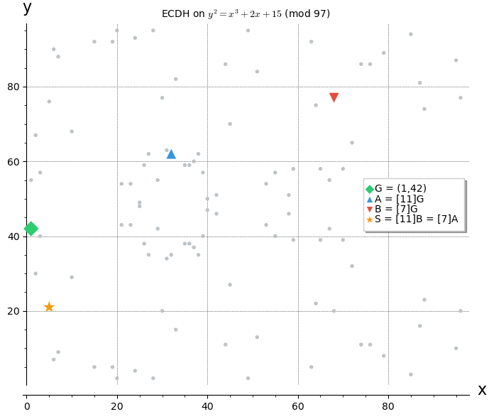
# -- Visualise ECDH on the curve using SageMath plotting --
p = 97; a_c = 2; b_c = 15
E = EllipticCurve(GF(p), [a_c, b_c])
G = E([1, 42])
n = G.order()

all_pts = E.rational_points()
affine_pts = [(ZZ(pt.xy()[0]), ZZ(pt.xy()[1])) for pt in all_pts if not pt.is_zero()]

# ECDH keys
a_priv_v = 11; b_priv_v = 7
A_pub_v = a_priv_v * G
B_pub_v = b_priv_v * G
S_v     = a_priv_v * B_pub_v

# Build plot
P_all = point2d(affine_pts, color='#bdc3c7', size=15, zorder=2)
P_G   = point2d([(ZZ(G.xy()[0]), ZZ(G.xy()[1]))],
                color='#2ecc71', size=120, marker='D', zorder=5,
                legend_label=f'G = ({G.xy()[0]},{G.xy()[1]})')
P_A   = point2d([(ZZ(A_pub_v.xy()[0]), ZZ(A_pub_v.xy()[1]))],
                color='#3498db', size=100, marker='^', zorder=5,
                legend_label=f'A = [{a_priv_v}]G')
P_B   = point2d([(ZZ(B_pub_v.xy()[0]), ZZ(B_pub_v.xy()[1]))],
                color='#e74c3c', size=100, marker='v', zorder=5,
                legend_label=f'B = [{b_priv_v}]G')
P_S   = point2d([(ZZ(S_v.xy()[0]), ZZ(S_v.xy()[1]))],
                color='#f39c12', size=160, marker='*', zorder=5,
                legend_label=f'S = [{a_priv_v}]B = [{b_priv_v}]A')

combined = P_all + P_G + P_A + P_B + P_S
combined.axes_labels(['x', 'y'])
show(combined,
     title=f'ECDH on $y^2 = x^3 + {a_c}x + {b_c}$ (mod {p})',
     figsize=(7, 6), gridlines=True)
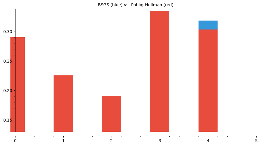
33.11 Attack Complexity Comparison#
Attack |
Complexity |
Requirement |
|---|---|---|
Brute force |
\(O(n)\) |
None |
Baby-step giant-step |
\(O(\sqrt{n})\) time & space |
Deterministic |
Pollard’s rho |
\(O(\sqrt{n})\) time, \(O(1)\) space |
Probabilistic |
Pohlig–Hellman |
\(O(\sum e_i(\log n + \sqrt{p_i}))\) |
Smooth order |
MOV attack |
\(L_{p^k}[1/3]\) |
Small embedding degree |
For a well-chosen curve (prime order \(n \approx 2^{256}\), large embedding degree), the best known attack is Pollard’s rho with \(\approx 2^{128}\) group operations.
# -- Compare BSGS vs Pohlig-Hellman on curves with different smoothness --
import time

test_data = [
    # (p, a, b, label)
    (101, 1, 6,  'p=101'),
    (97,  2, 15, 'p=97'),
    (131, 2, 3,  'p=131'),
    (157, 2, 3,  'p=157'),
    (199, 3, 7,  'p=199'),
]

labels = []
bsgs_times = []
ph_times   = []

for (pp, aa, bb, lbl) in test_data:
    Ei = EllipticCurve(GF(pp), [aa, bb])
    pts = Ei.rational_points()
    if len(pts) < 3:
        continue
    GG = pts[1]
    nn = GG.order()
    if nn < 5:
        continue
    k_test = nn // 2 + 1
    Qt = k_test * GG

    # BSGS timing
    t0 = time.perf_counter()
    bsgs_ec(GG, Qt, nn)
    bsgs_t = time.perf_counter() - t0

    # Pohlig-Hellman timing
    t0 = time.perf_counter()
    pohlig_hellman_ec(GG, Qt, nn)
    ph_t = time.perf_counter() - t0

    fac = factor(nn)
    largest = max(f[0] for f in fac)

    labels.append(f'{lbl}\nn={nn}\nmax_p={largest}')
    bsgs_times.append(bsgs_t * 1000)
    ph_times.append(ph_t * 1000)

# Display results as a table
print(f'{"Curve":>20s}  {"BSGS (ms)":>10s}  {"Pohlig-H (ms)":>14s}')
print('-' * 50)
for lbl, bt, pt in zip(labels, bsgs_times, ph_times):
    short_lbl = lbl.split('\n')[0]
    print(f'{short_lbl:>20s}  {float(bt):>10.3f}  {float(pt):>14.3f}')

# SageMath bar chart
x_pos = list(range(len(labels)))
bsgs_bar = bar_chart(bsgs_times, color='#3498db', width=0.4)
ph_bar   = bar_chart(ph_times,   color='#e74c3c', width=0.4)
show(bsgs_bar + ph_bar, title='BSGS (blue) vs. Pohlig-Hellman (red)', figsize=(9, 5))
               Curve   BSGS (ms)   Pohlig-H (ms)
--------------------------------------------------
               p=101       0.259           0.290
                p=97       0.189           0.225
               p=131       0.134           0.191
               p=157       0.193           0.334
               p=199       0.318           0.303
33.12 Exercises#
33.13 Summary#
This chapter implemented the cornerstone ECC protocols and the main classes of attack:
Topic |
Key takeaway |
|---|---|
Koblitz encoding |
Map messages to curve points via \(x = \kappa m + j\) |
ElGamal on EC |
Encryption via random \(k\); decryption via \(M_2 - sM_1\) |
ECDH |
Shared secret from scalar multiplication; 256-bit ECC \(\approx\) 3072-bit RSA |
ECDSA |
Sign = random nonce + scalar arithmetic; verify = two-scalar multi-mult |
Nonce reuse |
Reusing \(k\) leaks the private key in two signatures |
Pohlig–Hellman |
Smooth group order \(\Rightarrow\) trivial ECDLP |
Pollard’s rho |
Generic \(O(\sqrt{n})\) attack; sets the security baseline |
MOV attack |
Pairing-based reduction to finite-field DLP; foiled by large embedding degree |
Secure parameter selection requires:
Prime (or near-prime) group order to defeat Pohlig–Hellman.
Large embedding degree to defeat MOV.
Resistance to specialised attacks (anomalous curves, etc.).
Efficient arithmetic (e.g., curves over Mersenne-like primes).
References#
V. S. Miller, “Use of elliptic curves in cryptography,” CRYPTO 1985, LNCS 218, pp. 417–426, 1986.
N. Koblitz, “Elliptic curve cryptosystems,” Mathematics of Computation, vol. 48, no. 177, pp. 203–209, 1987.
A. Menezes, T. Okamoto, S. Vanstone, “Reducing elliptic curve logarithms to logarithms in a finite field,” IEEE Trans. Inf. Theory, vol. 39, no. 5, pp. 1639–1646, 1993.
D. Hankerson, A. Menezes, S. Vanstone, Guide to Elliptic Curve Cryptography, Springer, 2004.
NIST, “Recommended elliptic curves for federal government use,” FIPS 186-4, 2013 (updated FIPS 186-5, 2023).
J. M. Pollard, “Monte Carlo methods for index computation (mod \(p\)),” Mathematics of Computation, vol. 32, no. 143, pp. 918–924, 1978.
S. Pohlig, M. Hellman, “An improved algorithm for computing logarithms over \(GF(p)\) and its cryptographic significance,” IEEE Trans. Inf. Theory, vol. 24, no. 1, pp. 106–110, 1978.