
Chapter 5: The Vigenère Cipher and Kasiski Examination (SageMath)#
“A polyalphabetic cipher renders frequency analysis powerless — until one discovers the period.”
In the previous chapters we saw how monoalphabetic substitution ciphers are fundamentally vulnerable to frequency analysis: each plaintext letter is always mapped to the same ciphertext letter, so the statistical signature of the underlying language shines through. The Vigenère cipher was designed to defeat exactly this attack by cycling through multiple substitution alphabets, and for nearly three centuries it was considered unbreakable. In this chapter we study its design, formalize the notion of polyalphabetic substitution, and then demonstrate how Kasiski examination — a technique that exploits repeated patterns in ciphertext — recovers the key length and ultimately breaks the cipher.
Python Version Available
This notebook contains the SageMath implementation. A pure Python/NumPy version is available in Chapter 5: The Vigenere Cipher and Kasiski Test.
5.1 Historical Background#
5.1.1 Blaise de Vigenère and “Le Chiffre Indéchiffrable”#
The idea of using multiple cipher alphabets dates back to Leon Battista Alberti (c. 1467), but it was Blaise de Vigenère who, in his 1586 Traité des chiffres, described the mature form of the cipher that now bears his name. Earlier, in 1553, Giovan Battista Bellaso had published a similar scheme, and the attribution to Vigenère is historically debated. Nevertheless, the cipher became known as the Vigenère cipher and earned the reputation of “le chiffre indéchiffrable” — the indecipherable cipher.
The cipher’s strength lies in its polyalphabetic nature: rather than applying one fixed substitution, it cycles through \(L\) different Caesar shifts determined by a keyword of length \(L\). This flattens the frequency distribution of the ciphertext, making single-letter frequency analysis ineffective.
5.1.2 Babbage and Kasiski#
The Vigenère cipher resisted cryptanalysis for roughly 300 years. The first known break was accomplished by Charles Babbage around 1846, but he never published his work (possibly because the British government wished to keep the method secret during the Crimean War). Independently, the Prussian infantry officer Friedrich Wilhelm Kasiski published essentially the same technique in his 1863 book Die Geheimschriften und die Dechiffrir-Kunst (“Secret Writing and the Art of Deciphering”). The method is now universally known as the Kasiski examination.
Historical Note. Babbage’s unpublished notes, discovered much later, show he had cracked the Vigenère cipher as early as 1846 — seventeen years before Kasiski’s publication. This is one of several instances in the history of cryptanalysis where classified intelligence work anticipated published academic results.
5.2 Formal Definitions#
5.2.1 Polyalphabetic vs. Monoalphabetic Substitution#
Recall that a monoalphabetic substitution cipher uses a single permutation \(\pi: \mathbb{Z}_{26} \to \mathbb{Z}_{26}\) to encrypt every letter:
A polyalphabetic substitution cipher uses a family of permutations \(\{\pi_0, \pi_1, \ldots, \pi_{L-1}\}\), cycling through them with period \(L\):
The key distinction is that the same plaintext letter can map to different ciphertext letters depending on its position, which disrupts the frequency signature.
5.2.2 The Vigenère Cipher#
The Vigenère cipher is the special case where each \(\pi_j\) is a Caesar shift by \(k_j\):
Definition 5.1 (Vigenère Cipher). Let \(\mathbf{k} = (k_0, k_1, \ldots, k_{L-1}) \in \mathbb{Z}_{26}^L\) be a key of length \(L\). The Vigenère encryption of a plaintext message \(\mathbf{m} = (m_0, m_1, \ldots, m_{n-1})\) is:
\[E(m_i) = c_i = (m_i + k_{i \bmod L}) \bmod 26,\]and decryption is:
\[D(c_i) = m_i = (c_i - k_{i \bmod L}) \bmod 26.\]
Equivalently, we can think of the keyword as a string of letters (e.g., ENIGMA corresponds to \(\mathbf{k} = (4, 13, 8, 6, 12, 0)\)), and the encryption shifts each plaintext letter by the corresponding keyword letter.
5.2.3 The Kasiski Examination#
The Kasiski examination exploits the following observation: if the same plaintext trigram (or any \(n\)-gram) appears at two positions whose distance is a multiple of the key length \(L\), then it will be encrypted to the same ciphertext trigram. We can therefore search for repeated \(n\)-grams in the ciphertext, compute the distances between their occurrences, and take the GCD of those distances to estimate \(L\).
Definition 5.2 (Kasiski Examination). Given a ciphertext \(\mathbf{c}\), the Kasiski examination proceeds as follows:
Find all repeated \(n\)-grams (typically trigrams, \(n=3\)) in \(\mathbf{c}\).
For each repeated \(n\)-gram, compute the distances between all pairs of occurrences.
Compute the GCD of these distances. The result is likely a multiple of (or equal to) the key length \(L\).
5.3 Key Theoretical Results#
Theorem 5.1 (Kasiski’s Observation). Let \(\mathbf{m}\) be a plaintext and \(\mathbf{k}\) a Vigenère key of length \(L\). If a trigram \(m_i m_{i+1} m_{i+2}\) appears again at position \(j\) (i.e., \(m_j m_{j+1} m_{j+2} = m_i m_{i+1} m_{i+2}\)) and \(L \mid (j - i)\), then the corresponding ciphertext trigrams are identical:
\[c_i c_{i+1} c_{i+2} = c_j c_{j+1} c_{j+2}.\]
Proof. Since \(L \mid (j - i)\), we have \((j + r) \bmod L = (i + r) \bmod L\) for \(r = 0, 1, 2\). Therefore:
Corollary 5.1. The GCD of the distances between repeated ciphertext trigrams is likely a multiple of the key length \(L\). In practice, with sufficiently long ciphertext, the GCD often equals \(L\) exactly.
Caveat. Not every repeated ciphertext trigram arises from a repeated plaintext trigram at a distance divisible by \(L\). Coincidental repeats can occur. However, with longer ciphertext and more repeated \(n\)-grams, the statistical signal of the true key length dominates.
5.4 Implementation#
5.4.1 Vigenère Encrypt / Decrypt#
The following functions implement the Vigenère cipher using pure Python (no NumPy required in SageMath).
Algorithm for Vigenère Encryption:
Input the plaintext and the key.
Create a dictionary that maps each letter of the alphabet to its position.
Create an empty list to store the ciphertext.
Convert the key to lowercase.
Loop over each letter in the plaintext and encrypt it.
If the current character is not a letter, append it and continue.
Determine the index of the key letter to use (modulo key length).
Determine the index of the current plaintext letter.
Encrypt by adding the key index to the plaintext index, modulo 26.
Append the encrypted letter to the ciphertext list.
Convert the ciphertext list to a string and return it.
# Vigenere cipher -- SageMath implementation

import string
import re

def vigenere_encrypt(plaintext, key):
    """Encrypt plaintext with Vigenere cipher."""
    alphabet = string.ascii_lowercase
    letter_to_index = dict(zip(alphabet, range(len(alphabet))))
    ciphertext = []
    key = key.lower()

    for i, letter in enumerate(plaintext):
        if letter.lower() not in alphabet:
            ciphertext.append(letter)
            continue
        key_letter = key[i % len(key)]
        key_index = letter_to_index[key_letter]
        plaintext_index = letter_to_index[letter.lower()]
        ciphertext_letter = alphabet[(plaintext_index + key_index) % len(alphabet)]
        ciphertext.append(ciphertext_letter)

    return ''.join(ciphertext)


def vigenere_decrypt(ciphertext, key):
    """Decrypt ciphertext with Vigenere cipher."""
    alphabet = string.ascii_lowercase
    letter_to_index = dict(zip(alphabet, range(len(alphabet))))
    plaintext = []
    key = key.lower()

    for i, letter in enumerate(ciphertext):
        if letter.lower() not in alphabet:
            plaintext.append(letter)
            continue
        key_letter = key[i % len(key)]
        key_index = letter_to_index[key_letter]
        ciphertext_index = letter_to_index[letter.lower()]
        plaintext_letter = alphabet[(ciphertext_index - key_index) % len(alphabet)]
        plaintext.append(plaintext_letter)

    return ''.join(plaintext)

print("vigenere_encrypt / vigenere_decrypt loaded.")
vigenere_encrypt / vigenere_decrypt loaded.
# Remove all non-lowercase-letter characters
def lclear(text):
    return re.sub(r'[^a-z]', '', text.lower())

lalphabet = string.ascii_lowercase
print("lclear() loaded.  lalphabet =", lalphabet)
lclear() loaded. lalphabet = abcdefghijklmnopqrstuvwxyz
# Quick round-trip test
plaintext = lclear("hello world this is a short text to encrypt and decipher. "
                    "Notice that this is done in pure english. We write and we send, "
                    "this is our missions. Vignere cipher is safe, so they say. "
                    "However, I am not so sure anymore, is it?")
print("Plaintext: ", plaintext)

key = "enigma"
ciphertext = vigenere_encrypt(plaintext, key)
print("Ciphertext:", ciphertext)

decrypted_plaintext = vigenere_decrypt(ciphertext, key)
print("Decrypted: ", decrypted_plaintext)

assert decrypted_plaintext == plaintext, "Round-trip failed!"
print("\nEncrypt/Decrypt round-trip: OK")
Plaintext:  helloworldthisisashorttexttoencryptanddeciphernoticethatthisisdoneinpureenglishwewriteandwesendthisisourmissionsvignerecipherissafesotheysayhoweveriamnotsosureanymoreisit
Ciphertext: lrtrawsetjfhmfqymslbzzfebgbuqngegvfarqlkoitumxzoxvkkfhegbnusmfluzemaxadeiaorusljmcdixritpwifmtptlvaoeoyeuoesmbvyhikamxqcmcpkdiwfilqssgpkkselpuiezrzommrbbyasyemgzyqbzkusmg
Decrypted:  helloworldthisisashorttexttoencryptanddeciphernoticethatthisisdoneinpureenglishwewriteandwesendthisisourmissionsvignerecipherissafesotheysayhoweveriamnotsosureanymoreisit

Encrypt/Decrypt round-trip: OK
5.4.2 Index of Coincidence#
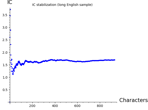
We use the index of coincidence (IC) to estimate the key length of a Vigenère cipher. The IC measures how likely it is that two randomly chosen letters from a text are the same. For English text, \(\mathrm{IC} \approx 1.73\) (when scaled by alphabet size 26), while for uniformly random text \(\mathrm{IC} \approx 1.0\).
When we split the ciphertext into \(L\) streams (one for each key position) and compute the IC of each stream, the correct key length \(L\) will produce streams whose IC is close to the English value.
def IC(sample, alphabet):
    """Compute the index of coincidence (scaled by alphabet size)."""
    s = lclear(sample)
    n = len(s)
    return float(len(alphabet) * sum([s.count(x) * (s.count(x) - 1)
                                       for x in alphabet]) / (n * (n - 1)))
# IC of ciphertext (should be closer to 1.0 -- random-like)
print("IC(ciphertext) =", IC(ciphertext, lalphabet))

# IC of plaintext (should be closer to 1.73 -- English-like)
print("IC(plaintext)  =", IC(plaintext, lalphabet))
IC(ciphertext) = 1.053393665158371
IC(plaintext)  = 1.860633484162896
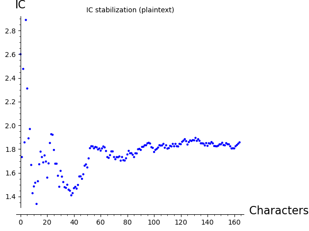
IC Stabilization#
As we include more text, the IC stabilizes toward its theoretical value. The following plots show this convergence for a long English sample and for our plaintext.
sample = '''This is the model used by many trade magazines (industry-based periodicals) distributed only to qualifying readers, often for free and determined by some form of survey. Because of costs (e.g., printing and postage) associated with the medium of print, publishers may not distribute free copies to everyone who requests one (unqualified leads); instead, they operate under controlled circulation, deciding who may receive free subscriptions based on each person's qualification as a member of the trade (and likelihood of buying, for example, likelihood of having corporate purchasing authority, as determined from job title). This allows a high level of certainty that advertisements will be received by the advertiser's target audience,[5] and it avoids wasted printing and distribution expenses. This latter model was widely used before the rise of the World Wide Web and is still employed by some titles. For example, in the United Kingdom, a number of computer-industry magazines use this model, including Computer Weekly and Computing, and in finance, Waters Magazine. For the global media industry, an example would be VideoAge International.'''

# IC stabilization for the long sample
list_plot([IC(sample[0:k], lalphabet) for k in range(5, len(lclear(sample)))],
          axes_labels=['Characters included', 'IC'],
          title='IC stabilization (long English sample)')
# IC stabilization for our plaintext
list_plot([IC(plaintext[0:k], lalphabet) for k in range(5, len(plaintext))],
          axes_labels=['Characters included', 'IC'],
          title='IC stabilization (plaintext)')
Using IC to Estimate Key Length#
If we split the ciphertext into streams by guessing key length \(L\), then for the correct \(L\) each stream is a simple Caesar cipher and its IC should be close to the English value (\(\approx 1.73\)). For incorrect guesses, letters from different shifts are mixed and the IC stays near \(1.0\).
# Subsequence extraction demo
a = 0
k = 3
N = len('123456789')
print("Every k-th character:", ''.join(['123456789'[k*i + a] for i in range(0, N // k)]))
Every k-th character: 147
# IC for different candidate key lengths (1 through 9)
N = len(ciphertext)

ic_by_length = [IC(''.join([ciphertext[kk*i] for i in range(0, N // kk)]), lalphabet)
                for kk in range(1, 10)]
print("IC values for candidate key lengths 1..9:")
for kk, ic_val in enumerate(ic_by_length, 1):
    marker = " <-- likely key length" if ic_val > 1.5 else ""
    print(f"  L={kk}: IC = {float(ic_val):.4f}{marker}")
IC values for candidate key lengths 1..9:
  L=1: IC = 1.0534
  L=2: IC = 1.3692
  L=3: IC = 1.1987
  L=4: IC = 1.9628 <-- likely key length
  L=5: IC = 0.9269
  L=6: IC = 1.5132 <-- likely key length
  L=7: IC = 0.4710
  L=8: IC = 1.3619
  L=9: IC = 0.6797
# Reference IC values
print("Random text IC (approx):", 1.9/26, "* 26 =", 0.0385*26)
print("English text IC (approx):", 0.0667*26)
Random text IC (approx): 0.0730769230769231 * 26 = 1.00100000000000
English text IC (approx): 1.73420000000000
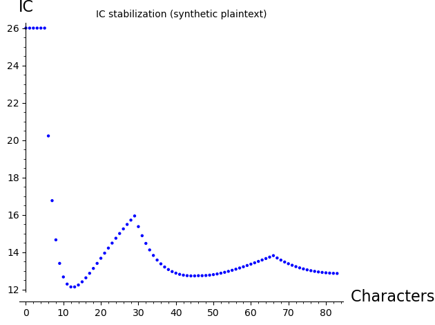
Synthetic Example#
One can apply the index of coincidence to a synthetic example. Notice how differently the IC stabilizes as we expand our context. How would you explain it?
# Synthetic example
plaintext2 = lclear("aaaaaaaabbbbbbbbaaaaaaaaaaaaaaaabbbbbbbbbbbbbbbbbaaaaaaaaaaaaaaaaaaaabbbbbbbbbbbbbbbbbb")
key2 = "confuse"
ciphertext2 = vigenere_encrypt(plaintext2, key2)
print("Ciphertext2:", ciphertext2)

decrypted_plaintext2 = vigenere_decrypt(ciphertext2, key2)
print("Decrypted2: ", decrypted_plaintext2)
Ciphertext2: confusecpogvtfdpnfuseconfuseconfvtfdpogvtfdpogvtfconfuseconfuseconfusfdpogvtfdpogvtfdpo
Decrypted2:  aaaaaaaabbbbbbbbaaaaaaaaaaaaaaaabbbbbbbbbbbbbbbbbaaaaaaaaaaaaaaaaaaaabbbbbbbbbbbbbbbbbb
# IC stabilization for synthetic plaintext
list_plot([IC(plaintext2[0:k], lalphabet) for k in range(3, len(lclear(plaintext2)))],
          axes_labels=['Characters included', 'IC'],
          title='IC stabilization (synthetic plaintext)')
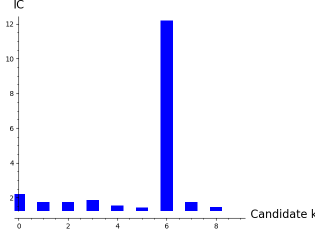
# IC per candidate key length for synthetic ciphertext
N = len(ciphertext2)
bar_chart([IC(''.join([ciphertext2[kk*i] for i in range(0, N // kk)]), lalphabet)
           for kk in range(1, 10)],
          axes_labels=['Candidate key length', 'IC'])
5.5 Experiments#
Experiment 1: Frequency Analysis#
Fails Against Vigenère
We encrypt a long English text with a Vigenère cipher (key length 5) and show that the single-letter frequency distribution of the ciphertext is nearly flat — far from the distinctive shape of English.
# --- Long English plaintext ---
long_text = (
    "Ciphers oh ciphers secrets they keep locked away in code deep and discreet "
    "symbols and numbers jumbled and mixed a message encoded ready to be fixed "
    "through history they have been used to hide plans of war love letters beside "
    "the Rosetta Stone a mystery solved a codebreakers work duly evolved "
    "from Caesar to Enigma through time they change yet the essence remains "
    "mysterious and strange a puzzle to solve a game to play a message to decipher "
    "in every way crack the code reveal the truth a challenge to minds sharp and "
    "astute for ciphers oh ciphers they hold the key to secrets untold waiting to "
    "be set free deep within the caves so dark and cold the dwarves they sat and "
    "stories told of treasure hoards and ancient lore and secrets kept for evermore "
    "but in their hands they held a tool a wondrous thing so sharp and cool "
    "a blade of steel that could carve letters and keep their secrets safe forever "
    "they used this tool to write their code a cipher strong that none could decode "
    "for every letter they would add another from their secret pad the Vigenere "
    "cipher was their art a thing of beauty a thing apart for only those who held "
    "the key could read the messages meant to be and so they wrote in cryptic lines "
    "their secrets safe from prying eyes for only those who knew the code could "
    "ever hope to share the load and though the world may never know the secrets "
    "kept so long ago the dwarves will always have their craft the Vigenere cipher "
    "strong and steadfast"
)

plaintext_long = lclear(long_text)
print(f"Plaintext length: {len(plaintext_long)} characters")

# Encrypt with key "flame" (length 5)
key_exp = "flame"
ciphertext_exp = vigenere_encrypt(plaintext_long, key_exp)
print(f"Key: '{key_exp}' (length {len(key_exp)})")
print(f"Ciphertext (first 80 chars): {ciphertext_exp[:80]}")

# --- Frequency analysis ---
def letter_frequencies(text, alphabet):
    """Compute letter frequency distribution."""
    n = len(text)
    return [float(text.count(ch)) / n for ch in alphabet]

plain_freq = letter_frequencies(plaintext_long, lalphabet)
cipher_freq = letter_frequencies(ciphertext_exp, lalphabet)

# Standard English frequencies
english_freq = [
    0.0817, 0.0150, 0.0278, 0.0425, 0.1270, 0.0223, 0.0202, 0.0609, 0.0697,
    0.0015, 0.0077, 0.0403, 0.0241, 0.0675, 0.0751, 0.0193, 0.0010, 0.0599,
    0.0633, 0.0906, 0.0276, 0.0098, 0.0236, 0.0015, 0.0197, 0.0007
]

# SageMath bar charts
G1 = bar_chart(english_freq, color='steelblue')
G2 = bar_chart(plain_freq, color='forestgreen')
G3 = bar_chart(cipher_freq, color='firebrick')

graphics_array([[G1, G2, G3]]).show(figsize=[16, 4])

print(f"\nPlaintext max frequency:  {float(max(plain_freq)):.4f}")
print(f"Ciphertext max frequency: {float(max(cipher_freq)):.4f}")
print("\nThe ciphertext frequencies are much flatter -- frequency analysis fails!")
Plaintext length: 1189 characters
Key: 'flame' (length 5)
Ciphertext (first 80 chars): htptiwdotgnahqvxdeovjesfljjkqiuwooojoaiedtnosipdqiulnphndcdijeskqgzleesongqgpren
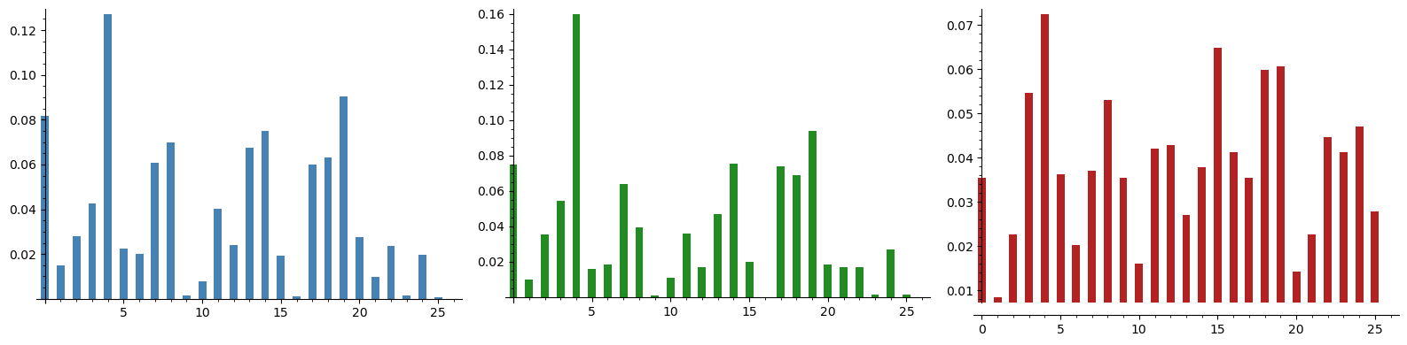
Plaintext max frequency:  0.1598
Ciphertext max frequency: 0.0723

The ciphertext frequencies are much flatter -- frequency analysis fails!
Observation. The Vigenère ciphertext has a much flatter frequency distribution than the plaintext. The standard deviation of ciphertext letter frequencies is roughly half that of plaintext frequencies, making it impossible to identify individual letters by frequency alone.
Experiment 2: Kasiski Examination Recovers the Key Length#
We now apply the Kasiski examination to the ciphertext. We find repeated trigrams, compute distances between their occurrences, and show that the GCD of these distances reveals the key length.
def find_substring_distance(s, n):
    """
    Find the distance between the first pair of identical substrings
    of length n. Returns -1 if no such substring is found.
    """
    substring_indices = {}
    for i in range(len(s) - n + 1):
        substring = s[i:i+n]
        if substring in substring_indices:
            return i - substring_indices[substring]
        else:
            substring_indices[substring] = i
    return -1

# Quick test
s = "abc1243654364872364782346823abcfkdjfkdjfdkabc"
print("Distance for trigrams in test string:", find_substring_distance(s, 3))
Distance for trigrams in test string: 4
# Apply Kasiski to the ciphertext encrypted with key "enigma" (length 6)
print("Distances for n-gram lengths 2..9:")
print([[find_substring_distance(ciphertext, k), k] for k in range(2, 10)])
Distances for n-gram lengths 2..9:
[[42, 2], [108, 3], [-1, 4], [-1, 5], [-1, 6], [-1, 7], [-1, 8], [-1, 9]]
# Full Kasiski examination on ciphertext_exp (key = "flame", length 5)

# Find repeated trigrams and their positions
trips = [ciphertext_exp[i:i+3] for i in range(0, len(ciphertext_exp) - 3)]
tripsd = {i: ciphertext_exp[i:i+3] for i in range(0, len(ciphertext_exp) - 3)}
repeated_trips = set([(x, trips.count(x)) for x in trips if trips.count(x) > 1])

print(f"Number of repeated trigrams: {len(repeated_trips)}")
print("\nSample repeated trigrams:")
for trigram, count in sorted(repeated_trips, key=lambda x: -x[1])[:10]:
    positions = [k for k in tripsd.keys() if tripsd[k] == trigram]
    print(f"  '{trigram}': count={count}, positions={positions}")
Number of repeated trigrams: 139

Sample repeated trigrams:
  'yse': count=10, positions=[285, 380, 474, 620, 630, 735, 850, 870, 985, 1120]
  'tti': count=8, positions=[137, 272, 712, 922, 937, 962, 1077, 1097]
  'xmp': count=6, positions=[459, 529, 539, 1034, 1144, 1154]
  'flj': count=6, positions=[23, 393, 508, 758, 813, 828]
  'lnp': count=5, positions=[51, 86, 546, 576, 626]
  'ehq': count=4, positions=[186, 451, 836, 1061]
  'hqv': count=4, positions=[12, 187, 362, 447]
  'nah': count=4, positions=[10, 360, 445, 511]
  'azh': count=4, positions=[312, 522, 957, 1177]
  'iwd': count=3, positions=[4, 439, 1169]
# Compute distances between repeated trigram occurrences
# and factor them using SageMath's ZZ().prime_factors()

outs_exp = [[[k for k in tripsd.keys() if tripsd[k] == f[0]], f[0]] for f in repeated_trips]

# Prime factorization of distances
pr_exp = [ZZ(x[0][1] - x[0][0]).prime_factors() for x in outs_exp if len(x[0]) >= 2]
print("Prime factors of trigram distances:")
print(pr_exp)

# Count factor frequencies
pprep = []
for el in pr_exp:
    pprep += el
factor_freq = [[x, pprep.count(x)] for x in sorted(list(set(pprep)))]
print("\nFactor frequency (factor, count):")
for f, c in factor_freq:
    marker = " <-- TRUE KEY LENGTH" if f == len(key_exp) else ""
    print(f"  {f}: {c}{marker}")
Prime factors of trigram distances:
[[2, 47], [3, 5, 29], [3, 5, 29], [2, 5, 79], [2, 5], [3, 5, 7], [2, 5, 11], [2, 5], [2, 3, 5], [5, 23], [2, 3, 5], [5, 7], [3, 5], [3, 5, 11], [2, 5], [3, 5], [2, 5, 11], [3, 5, 19], [2, 5], [2, 5, 7], [3, 5], [5, 13], [2, 5], [3, 5], [3, 5], [3, 5, 7], [2, 3, 5], [3, 5, 7], [3, 5, 7], [2, 3, 5], [2, 3, 17], [2, 3, 43], [3, 5, 7], [3, 5, 7], [3, 5, 13], [3, 163], [5], [2, 5, 37], [2, 3, 5, 31], [3, 5], [5, 11], [2, 5, 31], [2, 5, 17], [2, 3, 5], [2, 5], [3, 5, 29], [2, 5], [5, 53], [2, 5], [3, 5], [3, 5, 11], [2, 5, 7], [2, 5, 11], [5, 13], [2, 5], [5], [2, 5], [2, 3, 5], [2, 5, 7], [2, 5, 73], [3, 5, 11], [2, 5, 17], [5, 7], [3, 5, 13], [5, 173], [2, 5, 7], [5, 19], [2, 5, 11], [2, 5], [3, 5, 11], [2, 5], [5, 29], [2, 5], [3, 13], [5, 13], [2, 5, 17], [2, 5, 37], [2, 3, 5], [5, 11, 17], [5, 7], [2, 5, 7], [2, 5], [2, 5, 73], [3, 5, 29], [2, 5], [3, 5, 29], [2, 3, 5, 13], [2, 5, 11], [2, 5, 17], [3, 5, 7], [5, 7, 17], [2, 3, 5], [3, 5, 13], [2, 5], [2, 5], [2, 5], [5, 7, 11], [3, 5, 7], [2, 5], [5, 13], [3, 5, 29], [3, 5, 29], [2, 5], [307], [2, 5, 7], [2, 5], [3, 5, 7], [3, 5, 59], [5, 7], [2, 29], [3, 5, 11], [2, 3, 5], [2, 5], [3, 5, 7], [2, 3, 5], [2, 5, 7], [2, 5], [367], [3, 5, 29], [2, 5, 7], [2, 5], [2, 5], [2, 5, 59], [5], [2, 3, 5, 7], [5, 29], [2, 5, 59], [3, 5, 43], [2, 3, 5], [2, 5, 11], [5, 13], [3, 5, 29], [3, 5, 29], [199], [3, 5, 29], [3, 5, 43], [2, 3, 5, 7], [5, 7], [2, 3, 37]]

Factor frequency (factor, count):
  2: 71
  3: 60
  5: 129 <-- TRUE KEY LENGTH
  7: 27
  11: 14
  13: 10
  17: 7
  19: 2
  23: 1
  29: 14
  31: 2
  37: 3
  43: 3
  47: 1
  53: 1
  59: 3
  73: 2
  79: 1
  163: 1
  173: 1
  199: 1
  307: 1
  367: 1
# Also check doublets (bigrams) for more data points
doubles_exp = [ciphertext_exp[i:i+2] for i in range(0, len(ciphertext_exp) - 2)]
doublesd_exp = {i: ciphertext_exp[i:i+2] for i in range(0, len(ciphertext_exp) - 2)}
dd_exp = set([(x, doubles_exp.count(x)) for x in doubles_exp if doubles_exp.count(x) > 1])

outs_d = [[[k for k in doublesd_exp.keys() if doublesd_exp[k] == f[0]], f[0]] for f in dd_exp]
pr_d = [ZZ(x[0][1] - x[0][0]).prime_factors() for x in outs_d if len(x[0]) >= 2]

pprep_d = []
for el in pr_d:
    pprep_d += el
factor_freq_d = [[x, pprep_d.count(x)] for x in sorted(list(set(pprep_d)))]
print("Factor frequency from bigram distances:")
for f, c in factor_freq_d:
    marker = " <-- TRUE KEY LENGTH" if f == len(key_exp) else ""
    print(f"  {f}: {c}{marker}")
Factor frequency from bigram distances:
  2: 144
  3: 106
  5: 161 <-- TRUE KEY LENGTH
  7: 40
  11: 23
  13: 20
  17: 12
  19: 10
  23: 13
  29: 13
  31: 2
  37: 4
  41: 8
  43: 6
  47: 2
  53: 4
  59: 4
  61: 2
  67: 4
  71: 3
  73: 1
  79: 5
  89: 2
  97: 2
  101: 1
  107: 1
  113: 1
  127: 1
  131: 1
  149: 2
  151: 2
  157: 3
  167: 1
  179: 1
  181: 2
  191: 1
  199: 1
  223: 1
  229: 1
  241: 1
  269: 1
  281: 1
  307: 2
  331: 1
  337: 1
  379: 1
  383: 1
  401: 1
  409: 1
  461: 1
  491: 1
  587: 1
  593: 1
  743: 1
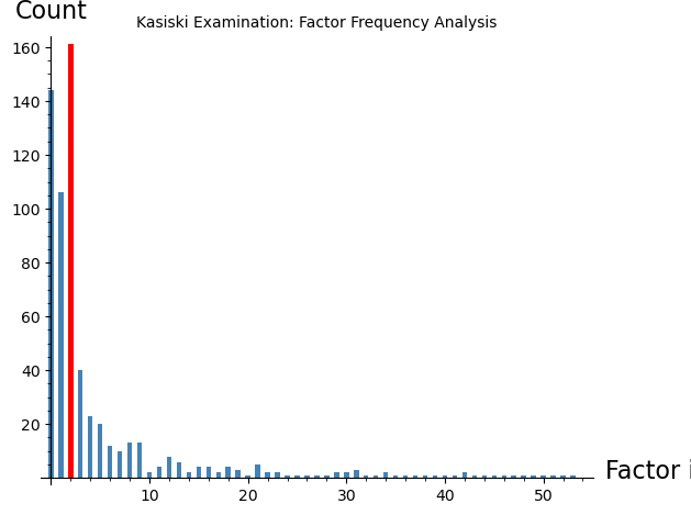
# Visualize factor frequency as a bar chart
factors = [f for f, c in factor_freq_d]
counts = [c for f, c in factor_freq_d]
colors = ['red' if f == len(key_exp) else 'steelblue' for f in factors]

bar_chart(counts, color=colors,
          axes_labels=['Factor index', 'Count'],
          title='Kasiski Examination: Factor Frequency Analysis')
Experiment 3: Splitting Ciphertext into \(L\) Streams#
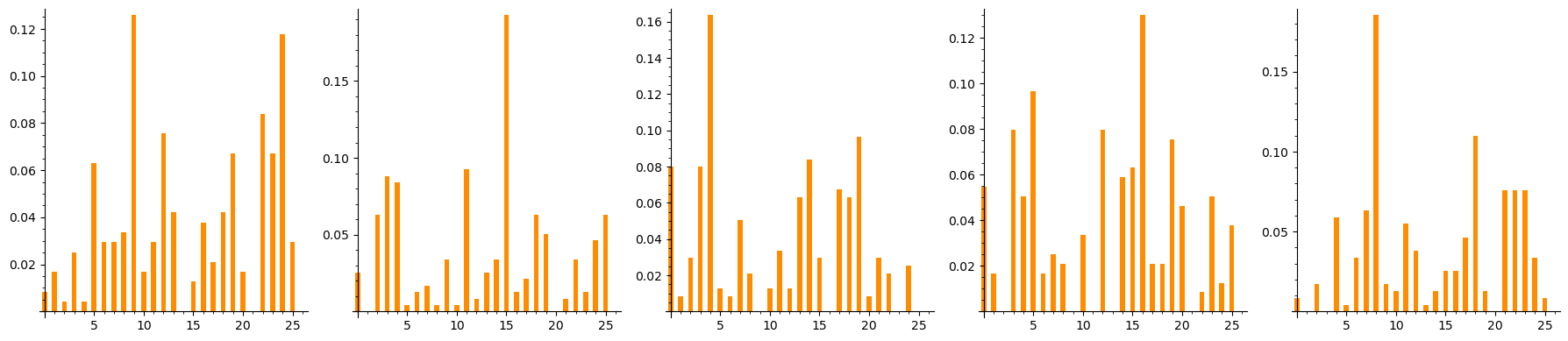
Once the key length \(L\) is known (or guessed), we can split the ciphertext into \(L\) independent streams. Stream \(j\) consists of every \(L\)-th character starting from position \(j\):
Each stream has been encrypted with a single Caesar shift \(k_j\), so we can apply frequency analysis to each stream independently.
# Split ciphertext into L=5 streams
L = 5  # key length from Kasiski examination

streams = [ciphertext_exp[j::L] for j in range(L)]

print(f"Ciphertext length: {len(ciphertext_exp)}")
print(f"Key length L = {L}")
for j, s in enumerate(streams):
    print(f"  Stream {j}: {len(s)} chars, first 30: '{s[:30]}'")
Ciphertext length: 1189
Key length L = 5
  Stream 0: 238 chars, first 30: 'hwnxjjujdiunjgsgzinrltjtcwmwdg'
  Stream 1: 238 chars, first 30: 'tdadejwotpldezopxlippolmpztjsp'
  Stream 2: 238 chars, first 30: 'poheskoandncslnrbneseededustae'
  Stream 3: 238 chars, first 30: 'ttqofqoioqpdkegexppezpkrfsfthz'
  Stream 4: 237 chars, first 30: 'igvvlioesihiqeqniqeegvxmllsiiy'
# Frequency distributions of individual streams (SageMath bar charts)
plots = []
for j in range(L):
    stream = streams[j]
    freq = [float(stream.count(ch)) / len(stream) for ch in lalphabet]
    p = bar_chart(freq, color='darkorange')
    plots.append(p)

graphics_array([plots]).show(figsize=[18, 4])
print("Each stream shows a shifted version of the English frequency distribution!")
Each stream shows a shifted version of the English frequency distribution!
Key Insight. Each individual stream is just a Caesar cipher! The frequency distribution of each stream is a shifted copy of the English frequency distribution. We can recover the shift (and thus the corresponding key letter) by finding which shift maximizes the correlation with the standard English frequencies.
Experiment 4: Full Attack#
Pipeline
We now implement the complete attack: Kasiski examination determines the key length, then frequency analysis on each stream recovers each key letter, and finally we decrypt the message.
# --- Full Vigenere Attack Pipeline (SageMath) ---

def Frequency(text, alphabet):
    """Compute letter frequency distribution."""
    s = lclear(text)
    return [float(s.count(let)) / len(s) for let in alphabet]

def chi_squared_score(observed, expected):
    """Compute chi-squared statistic."""
    return sum([(observed[i] - expected[i])^2 / expected[i]
                for i in range(len(expected)) if expected[i] > 0])

def recover_shift(stream_text):
    """Determine the Caesar shift for a single stream."""
    best_shift = 0
    best_score = Infinity
    for shift in range(26):
        decrypted = ''.join([chr(ord('a') + (ord(ch) - ord('a') - shift) % 26)
                             for ch in stream_text])
        freq = Frequency(decrypted, lalphabet)
        score = chi_squared_score(freq, english_freq)
        if score < best_score:
            best_score = score
            best_shift = shift
    return best_shift

print("=" * 60)
print("FULL VIGENERE ATTACK PIPELINE (SageMath)")
print("=" * 60)
print(f"\nStep 1: Key length from Kasiski examination: L = {L}")

recovered_key = []
print(f"\nStep 2: Recovering key letters via frequency analysis:")
for j in range(L):
    stream = ciphertext_exp[j::L]
    shift = recover_shift(stream)
    key_letter = chr(shift + ord('a'))
    recovered_key.append(key_letter)
    print(f"  Stream {j}: best shift = {int(shift):2d} -> key letter = '{key_letter}'")

recovered_key_str = ''.join(recovered_key)
print(f"\nRecovered key: '{recovered_key_str}'")
print(f"Actual key:    '{key_exp}'")
print(f"Key recovery:  {'SUCCESS' if recovered_key_str == key_exp else 'PARTIAL'}")

# --- Step 3: Decrypt ---
decrypted_text = vigenere_decrypt(ciphertext_exp, recovered_key_str)
print(f"\nStep 3: Decrypted text (first 200 chars):")
print(f"  {decrypted_text[:200]}")
print(f"\nDecryption matches original plaintext: {decrypted_text == plaintext_long}")
============================================================
FULL VIGENERE ATTACK PIPELINE (SageMath)
============================================================

Step 1: Key length from Kasiski examination: L = 5

Step 2: Recovering key letters via frequency analysis:
  Stream 0: best shift =  5 -> key letter = 'f'
  Stream 1: best shift = 11 -> key letter = 'l'
  Stream 2: best shift =  0 -> key letter = 'a'
  Stream 3: best shift = 12 -> key letter = 'm'
  Stream 4: best shift =  4 -> key letter = 'e'

Recovered key: 'flame'
Actual key:    'flame'
Key recovery:  SUCCESS

Step 3: Decrypted text (first 200 chars):
  ciphersohcipherssecretstheykeeplockedawayincodedeepanddiscreetsymbolsandnumbersjumbledandmixedamessageencodedreadytobefixedthroughhistorytheyhavebeenusedtohideplansofwarlovelettersbesidetherosettaston

Decryption matches original plaintext: True
Complete Break. The Vigenère cipher, once considered unbreakable, falls to a two-stage attack:
Kasiski examination reveals the key length \(L\) from repeated ciphertext patterns.
Frequency analysis on each of the \(L\) Caesar-cipher streams recovers each key letter.
The entire attack requires only the ciphertext (a ciphertext-only attack) and knowledge that the underlying language is English.
Experiment 5: A Complete Attack on a Different Key#
We demonstrate the full attack pipeline end-to-end on a ciphertext encrypted with the key "hunter" (length 6). This follows the user’s original SageMath attack workflow using ZZ, factor(), and gcd().
poem = '''Ciphers, oh ciphers, secrets they keep
Locked away in code, deep and discreet
Symbols and numbers, jumbled and mixed
A message encoded, ready to be fixed

Through history they've been used to hide
Plans of war, love letters beside
The Rosetta Stone, a mystery solved
A codebreaker's work, duly evolved

From Caesar to Enigma, through time they change
Yet the essence remains, mysterious and strange
A puzzle to solve, a game to play
A message to decipher, in every way

Crack the code, reveal the truth
A challenge to minds, sharp and astute
For ciphers, oh ciphers, they hold the key
To secrets untold, waiting to be set free.'''

plaintext_poem = lclear(poem)
key5 = "hunter"  # six letters
ciphertext5 = vigenere_encrypt(plaintext_poem, key5)

print("First substring distances:")
print([[find_substring_distance(ciphertext5, k), k] for k in range(2, 20)])

# Find repeated trigrams
trips5 = [ciphertext5[i:i+3] for i in range(0, len(ciphertext5) - 3)]
tripsd5 = {i: ciphertext5[i:i+3] for i in range(0, len(ciphertext5) - 3)}
tt5 = set([(x, trips5.count(x)) for x in trips5 if trips5.count(x) > 1])
print("\nRepeated trigrams:", tt5)
First substring distances:
[[12, 2], [18, 3], [114, 4], [348, 5], [348, 6], [-1, 7], [-1, 8], [-1, 9], [-1, 10], [-1, 11], [-1, 12], [-1, 13], [-1, 14], [-1, 15], [-1, 16], [-1, 17], [-1, 18], [-1, 19]]

Repeated trigrams: {('nux', 3), ('yel', 3), ('koy', 3), ('lnb', 2), ('bli', 2), ('rms', 2), ('ika', 2), ('iiz', 2), ('oye', 2), ('ekm', 2), ('tru', 2), ('abr', 2), ('lik', 2), ('vmg', 2), ('mgo', 2), ('brv', 2), ('gyh', 2), ('goy', 2), ('wko', 2), ('oyl', 3), ('sul', 2), ('lll', 2)}
# Positions and prime factors of trigram distances
outs5 = [[[k for k in tripsd5.keys() if tripsd5[k] == f[0]], f[0]] for f in tt5]
print("Trigram positions:")
print(outs5)

print("\nPrime factors of distances:")
print([ZZ(x[0][1] - x[0][0]).prime_factors() for x in outs5 if len(x[0]) >= 2])
Trigram positions:
[[[283, 391, 457], 'nux'], [[13, 175, 223], 'yel'], [[23, 137, 449], 'koy'], [[263, 408], 'lnb'], [[188, 464], 'bli'], [[326, 338], 'rms'], [[172, 190], 'ika'], [[4, 76], 'iiz'], [[12, 360], 'oye'], [[311, 413], 'ekm'], [[51, 69], 'tru'], [[270, 378], 'abr'], [[189, 489], 'lik'], [[9, 357], 'vmg'], [[10, 358], 'mgo'], [[363, 379], 'brv'], [[274, 400], 'gyh'], [[11, 359], 'goy'], [[22, 448], 'wko'], [[24, 138, 450], 'oyl'], [[342, 382], 'sul'], [[204, 205], 'lll']]

Prime factors of distances:
[[2, 3], [2, 3], [2, 3, 19], [5, 29], [2, 3, 23], [2, 3], [2, 3], [2, 3], [2, 3, 29], [2, 3, 17], [2, 3], [2, 3], [2, 3, 5], [2, 3, 29], [2, 3, 29], [2], [2, 3, 7], [2, 3, 29], [2, 3, 71], [2, 3, 19], [2, 5], []]
# Doublet (bigram) analysis for more evidence
doubles5 = [ciphertext5[i:i+2] for i in range(0, len(ciphertext5) - 2)]
doublesd5 = {i: ciphertext5[i:i+2] for i in range(0, len(ciphertext5) - 2)}
dd5 = set([(x, doubles5.count(x)) for x in doubles5 if doubles5.count(x) > 1])

outs52 = [[[k for k in doublesd5.keys() if doublesd5[k] == f[0]], f[0]] for f in dd5]

pr5 = [ZZ(x[0][1] - x[0][0]).prime_factors() for x in outs52 if len(x[0]) >= 2]
print("Prime factors from bigram distances:")
print(pr5)

pprep = []
for el in pr5:
    pprep += el
factor_counts_5 = [[x, pprep.count(x)] for x in sorted(list(set(pprep)))]
print("\nFactor frequency:")
for f, c in factor_counts_5:
    print(f"  {f}: {c}")
print("\nConclusion: the most likely key length is 6")
Prime factors from bigram distances:
[[11, 13], [2, 3, 17], [2, 3, 5], [3, 101], [7, 17], [2, 5], [151], [2, 3, 7], [2, 61], [3], [2, 3, 7], [79], [2, 11], [17], [2, 3, 53], [2, 3, 13], [2, 71], [3, 41], [2, 3], [2], [13], [2, 3, 11], [2, 3], [2, 3, 19], [199], [2, 3], [3, 23], [2, 3], [3, 37], [2, 3, 5], [2, 5, 13], [2, 5, 11], [227], [5, 19], [3, 13], [3, 19], [7, 29], [2], [2, 89], [2, 7], [2, 3, 5], [109], [2, 3], [3, 5, 23], [2, 3, 7], [2, 3], [2], [2, 13], [2, 3, 19], [2, 5, 7], [401], [2, 3, 17], [2, 3, 5], [2, 3, 11], [3, 11], [2, 3, 23], [2, 61], [2, 13], [2, 3], [2, 17], [2, 5], [2, 11], [2, 3], [2, 3, 13], [2, 3, 5, 7], [2, 3, 7], [2, 3], [2, 3], [], [2, 3], [3, 5], [2, 3, 17], [3, 31], [2, 3], [2, 7, 11], [263], [2, 3, 7], [2, 3], [2, 3], [2, 67], [2, 3], [2, 3], [5, 13], [5, 37], [2, 3], [13, 19], [2, 3, 11], [113], [109], [2, 3], [2, 3, 41], [2, 3], [2, 3, 7], [2, 3, 41], [13], [2, 3], [2, 3, 23], [2, 3, 29], [2, 3], [11], [97], [2, 3, 17], [2, 5, 11], [2, 3, 71], [3], [2, 3], [2, 3, 29], [2, 3, 13], [11, 29], [2, 3, 7], [2, 7, 23]]

Factor frequency:
  2: 76
  3: 66
  5: 16
  7: 14
  11: 12
  13: 12
  17: 7
  19: 5
  23: 5
  29: 4
  31: 1
  37: 2
  41: 3
  53: 1
  61: 2
  67: 1
  71: 2
  79: 1
  89: 1
  97: 1
  101: 1
  109: 2
  113: 1
  151: 1
  199: 1
  227: 1
  263: 1
  401: 1

Conclusion: the most likely key length is 6
Applying Frequency Analysis to Find the Key Letters#
Once we have established the key length, we apply frequency analysis to find the exact key. We split the ciphertext into 6 streams and find the most common letter in each. Since ‘e’ is the most common English letter, the most frequent ciphertext letter in each stream likely corresponds to ‘e’ shifted by the key letter.
# Split into 6 streams and recover key via chi-squared scoring
letlist = [ciphertext5[k::6] for k in range(6)]

# Recover each key letter using chi-squared (more robust than most-common-letter)
print("Key recovery by frequency analysis:")
print("=" * 50)
recovered = []
for j in range(6):
    stream = letlist[j]
    shift = recover_shift(stream)
    key_letter = chr(shift + ord('a'))
    recovered.append(key_letter)
    print(f"  Stream {j}: length = {len(stream)}, "
          f"best shift = {int(shift):2d} -> key letter = '{key_letter}'")

print(f"\nRecovered key: '{''.join(recovered)}'")
print(f"Actual key:    '{key5}'")
print(f"Match: {''.join(recovered) == key5}")
Key recovery by frequency analysis:
==================================================
  Stream 0: length = 83, best shift =  7 -> key letter = 'h'
  Stream 1: length = 83, best shift = 20 -> key letter = 'u'
  Stream 2: length = 83, best shift = 13 -> key letter = 'n'
  Stream 3: length = 83, best shift = 19 -> key letter = 't'
  Stream 4: length = 82, best shift =  4 -> key letter = 'e'
  Stream 5: length = 82, best shift = 17 -> key letter = 'r'

Recovered key: 'hunter'
Actual key:    'hunter'
Match: True
Experiment 6: Effect of Key Length on Security#
How does the key length affect the difficulty of the Kasiski attack? Longer keys produce fewer repeated trigrams, making the examination harder. We test multiple key lengths and track the number of repeated trigrams.
# Test multiple key lengths
test_keys = {
    2: "ab",
    3: "key",
    4: "code",
    5: "flame",
    6: "hunter",
    7: "richard",
    8: "security",
    10: "encryption",
    12: "cryptography",
}

results = []
for L_test, k_test in sorted(test_keys.items()):
    ct = vigenere_encrypt(plaintext_long, k_test)

    # Count repeated trigrams
    ngram_pos = {}
    for i in range(len(ct) - 2):
        ng = ct[i:i+3]
        if ng not in ngram_pos:
            ngram_pos[ng] = []
        ngram_pos[ng].append(i)
    repeated = {ng: pos for ng, pos in ngram_pos.items() if len(pos) > 1}
    n_repeated = len(repeated)

    results.append((L_test, n_repeated))
    print(f"Key length {int(L_test):2d} ('{k_test:12s}'): {int(n_repeated):3d} repeated trigrams")

# Plot using SageMath list_plot
list_plot(results, plotjoined=True, marker='o', color='steelblue',
          axes_labels=['Key length $L$', 'Repeated trigrams'],
          title='Effect of Key Length on Kasiski Examination',
          figsize=[9, 5])
Key length  2 ('ab          '): 206 repeated trigrams
Key length  3 ('key         '): 185 repeated trigrams
Key length  4 ('code        '): 176 repeated trigrams
Key length  5 ('flame       '): 140 repeated trigrams
Key length  6 ('hunter      '): 132 repeated trigrams
Key length  7 ('richard     '): 148 repeated trigrams
Key length  8 ('security    '): 138 repeated trigrams
Key length 10 ('encryption  '): 110 repeated trigrams
Key length 12 ('cryptography'): 104 repeated trigrams
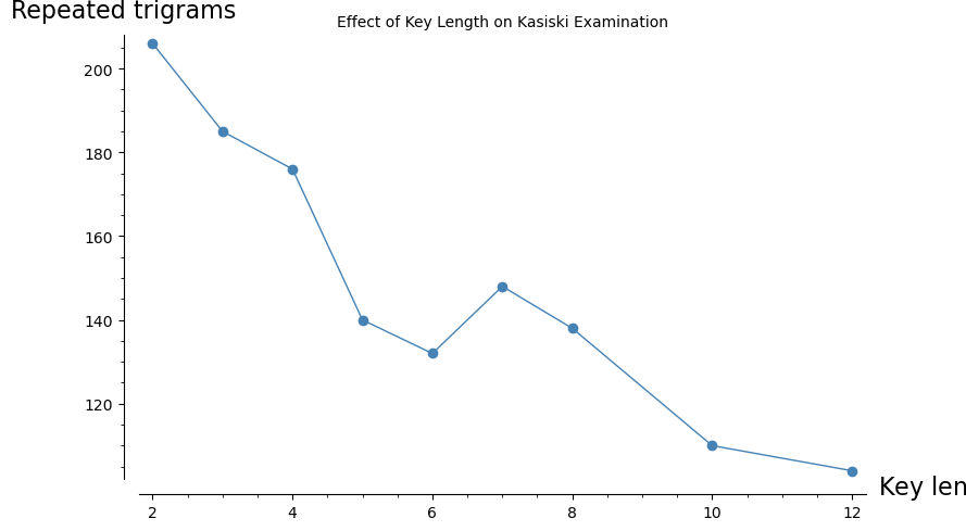
Observation. As the key length increases, the number of repeated trigrams decreases.
For very long keys (approaching the length of the plaintext), the cipher becomes a one-time pad and is theoretically unbreakable. In practice, the Kasiski method works well for key lengths up to about 10–15 with texts of a few hundred characters.
Experiment 7: Kasiski with Short Keys#
Let us explore the Kasiski method with short keys where the pattern is especially clear.
# Key "abcd" (length 4) -- very clear Kasiski pattern
key_short = "abcd"
ct_short = vigenere_encrypt(plaintext, key_short)

print("Substring distances for key 'abcd':")
print([[find_substring_distance(ct_short, k), k] for k in range(2, 20)])

# Find repeated trigrams
trips_s = [ct_short[i:i+3] for i in range(0, len(ct_short) - 3)]
tripsd_s = {i: ct_short[i:i+3] for i in range(0, len(ct_short) - 3)}
tt_s = set([(x, trips_s.count(x)) for x in trips_s if trips_s.count(x) > 1])
print("\nRepeated trigrams:", tt_s)
Substring distances for key 'abcd':
[[4, 2], [20, 3], [-1, 4], [-1, 5], [-1, 6], [-1, 7], [-1, 8], [-1, 9], [-1, 10], [-1, 11], [-1, 12], [-1, 13], [-1, 14], [-1, 15], [-1, 16], [-1, 17], [-1, 18], [-1, 19]]

Repeated trigrams: {('kvi', 2), ('juv', 2), ('prt', 2)}
# Positions and factorizations of repeated trigram distances
for trigram, count in sorted(tt_s, key=lambda x: -x[1])[:5]:
    positions = [k for k in tripsd_s.keys() if tripsd_s[k] == trigram]
    if len(positions) >= 2:
        dist = positions[1] - positions[0]
        print(f"'{trigram}': positions={positions}, distance={dist}, factors={ZZ(dist).factor()}")
'kvi': positions=[58, 166], distance=108, factors=2^2 * 3^3
'juv': positions=[105, 125], distance=20, factors=2^2 * 5
'prt': positions=[46, 150], distance=104, factors=2^3 * 13
# Key "abcde" (length 5)
key_5 = "abcde"
ct_5 = vigenere_encrypt(plaintext, key_5)

trips3 = [ct_5[i:i+3] for i in range(0, len(ct_5) - 3)]
tripsd3 = {i: ct_5[i:i+3] for i in range(0, len(ct_5) - 3)}
tt3 = set([(x, trips3.count(x)) for x in trips3 if trips3.count(x) > 1])

outs3 = [[[k for k in tripsd3.keys() if tripsd3[k] == f[0]], f[0]] for f in tt3]
print("Positions of repeated trigrams for key 'abcde':")
print(outs3)

# Distances and their GCD
distances = [x[0][1] - x[0][0] for x in outs3 if len(x[0]) >= 2]
print("\nDistances:", distances)
if len(distances) >= 2:
    print("GCD:", gcd(distances))
Positions of repeated trigrams for key 'abcde':
[[[10, 95], 'tik'], [[11, 96], 'ikv'], [[12, 97], 'kvm'], [[105, 125], 'itu'], [[9, 94], 'hti'], [[13, 98], 'vms']]

Distances: [85, 85, 85, 20, 85, 85]
GCD: 5
# Key "richard" (length 7) -- using SageMath factor()
key_7 = "richard"
ct_7 = vigenere_encrypt(plaintext, key_7)

doubles4 = [ct_7[i:i+2] for i in range(0, len(ct_7) - 2)]
doublesd4 = {i: ct_7[i:i+2] for i in range(0, len(ct_7) - 2)}
dd4 = set([(x, doubles4.count(x)) for x in doubles4 if doubles4.count(x) > 1])

outs = [[[k for k in doublesd4.keys() if doublesd4[k] == f[0]], f[0]] for f in dd4]

# Prime factor analysis using SageMath
pr = [ZZ(x[0][1] - x[0][0]).prime_factors() for x in outs if len(x[0]) >= 2]
print("Prime factors of bigram distances for key 'richard':")
print(pr)

pprep = []
for el in pr:
    pprep += el
print("\nFactor frequency:")
print([[x, pprep.count(x)] for x in sorted(list(set(pprep)))])
Prime factors of bigram distances for key 'richard':
[[2, 3, 7], [2, 7], [2, 7, 11], [3, 5], [7], [3, 7], [2], [2, 3], [73], [13], [17], [3, 13], [3, 5], [2, 11], [7, 11], [7, 13], [7], [2, 11], [5, 29], [2, 3, 7], [23], [2, 7, 11], [2, 29], [7, 13]]

Factor frequency:
[[2, 10], [3, 7], [5, 3], [7, 11], [11, 5], [13, 4], [17, 1], [23, 1], [29, 2], [73, 1]]
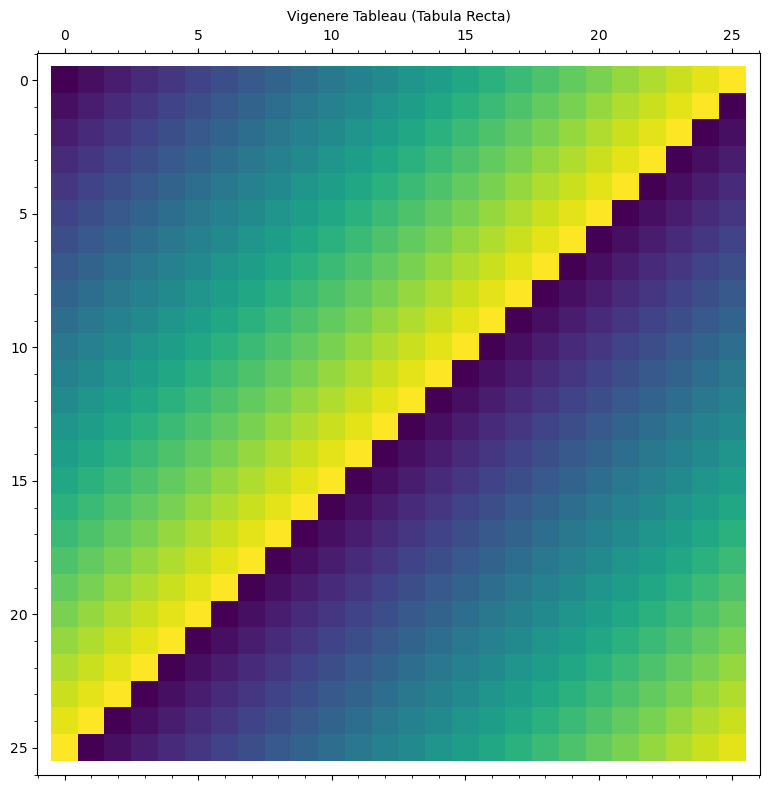
Experiment 8: Visualizing the Vigenère Tableau#
The classical Vigenère tableau (or tabula recta) is a \(26 \times 26\) table where row \(i\) is the alphabet shifted by \(i\) positions. We visualize it as a heatmap using SageMath’s matrix_plot.
# Build and visualize the Vigenere tableau
tableau = matrix(ZZ, 26, 26, lambda i, j: (i + j) % 26)

matrix_plot(tableau, cmap='viridis', figsize=[9, 8],
            title='Vigenere Tableau (Tabula Recta)')
5.6 Exercises#
Exercise 5.1 (Manual Vigenère). Encrypt the plaintext
ATTACKATDAWNwith the Vigenère keyLEMONby hand, using the Vigenère tableau. Verify your result with thevigenere_encryptfunction.
Exercise 5.2 (Kasiski by Hand). Given the ciphertext below (encrypted with a Vigenère cipher of unknown key length), find all repeated trigrams and their distances. What key length does the Kasiski examination suggest?
Ciphertext:
VVHQWVVRHMUSGJGTHKIHTSSEJCHLSFCBGVWCRLRYQTFSVGAHWKCUHWAUGLQHNSLRLJSHBLTSPISPRDXLJSVEEGHLQWKASSKUWEPHint: Look for trigrams that appear at least twice and compute the GCD of all distances.
Exercise 5.3 (Chi-Squared vs. Dot Product). In the key-recovery step, we used the chi-squared statistic to measure how well a candidate shift matches the expected English frequencies. An alternative is the dot product (or correlation) method:
\[\text{score}(s) = \sum_{i=0}^{25} f_i \cdot e_{(i - s) \bmod 26}\]where \(f_i\) is the frequency of letter \(i\) in the stream and \(e_j\) is the expected English frequency of letter \(j\). Implement this alternative and compare the results. Which method is more robust with short texts?
Exercise 5.4 (Key Length vs. Text Length). Experimentally determine the minimum ciphertext length needed for a successful Kasiski attack as a function of key length. For key lengths \(L = 3, 4, 5, \ldots, 12\), find the shortest prefix of the ciphertext for which the Kasiski examination correctly identifies \(L\). Plot your results using
list_plot().
Exercise 5.5 (Autokey Cipher). The autokey cipher (also attributed to Vigenère) uses the plaintext itself to extend the key:
\[\begin{split}c_i = (m_i + k_i) \bmod 26, \quad \text{where } k_i = \begin{cases} \text{keyword}[i] & \text{if } i < L, \\ m_{i - L} & \text{if } i \geq L. \end{cases}\end{split}\]Implement the autokey cipher. Explain why the Kasiski examination does not work against it. What alternative attack strategies might apply?
5.7 Summary#
In this chapter we studied the Vigenère cipher and its cryptanalysis via the Kasiski examination:
Concept |
Key Point |
|---|---|
Vigenère cipher |
Polyalphabetic substitution: \(c_i = (m_i + k_{i \bmod L}) \bmod 26\) |
Polyalphabetic advantage |
Same plaintext letter maps to different ciphertext letters, flattening frequency distributions |
Index of coincidence |
IC \(\approx 1.73\) for English, \(\approx 1.0\) for random; use per-stream IC to identify correct key length |
Kasiski examination |
Repeated ciphertext \(n\)-grams reveal the key length via GCD of distances |
SageMath tools |
|
Theorem 5.1 |
If \(L \mid (j-i)\) and plaintext trigrams at \(i, j\) are equal, then ciphertext trigrams at \(i, j\) are equal |
Stream decomposition |
Once \(L\) is known, split into \(L\) Caesar streams and apply frequency analysis independently |
Full attack |
Ciphertext-only: Kasiski \(\to\) key length \(\to\) frequency analysis per stream \(\to\) key recovery \(\to\) decryption |
Limitations |
Longer keys require longer ciphertext; very long keys approach one-time-pad security |
Looking Ahead. In Chapter 6, we will study the index of coincidence (Friedman, 1922) in greater depth, which provides a more systematic and robust method for determining the key length of a polyalphabetic cipher. Unlike Kasiski examination, which relies on finding repeated \(n\)-grams, the index of coincidence uses a global statistical measure.
5.8 References#
Vigenère, B. (1586). Traité des chiffres, ou secrètes manières d’escrire. Paris.
Kasiski, F. W. (1863). Die Geheimschriften und die Dechiffrir-Kunst. Berlin: E. S. Mittler und Sohn.
Babbage, C. (c. 1846). Unpublished notes on breaking the Vigenère cipher, held in the British Library.
Singh, S. (1999). The Code Book: The Science of Secrecy from Ancient Egypt to Quantum Cryptography. Anchor Books. Chapter 2.
Katz, J. and Lindell, Y. (2020). Introduction to Modern Cryptography. 3rd ed. CRC Press. Section 1.3.
Stinson, D. R. and Paterson, M. (2018). Cryptography: Theory and Practice. 4th ed. CRC Press. Chapter 2.
Friedman, W. F. (1922). The Index of Coincidence and Its Applications in Cryptanalysis. Department of Ciphers, Riverbank Laboratories, Publication No. 22.