Chapter 14: Block Cipher

Design (SageMath)

Python Version Available

This notebook contains the SageMath implementation. A pure Python/NumPy version is available in Chapter 14: Block Cipher Design.

14.1 Historical Context

The design of modern block ciphers rests on a foundation laid over several decades by a small number of remarkably influential thinkers.

Claude Shannon (1949). In his landmark paper Communication Theory of Secrecy Systems, Shannon introduced two properties that every strong cipher should possess: confusion and diffusion. Confusion obscures the relationship between the key and the ciphertext, while diffusion spreads the influence of each plaintext bit across the entire ciphertext. Shannon observed that simple substitution provides confusion and simple transposition provides diffusion, and he proposed that a product cipher – one that alternates substitution and transposition layers – could achieve both properties simultaneously. This insight is the intellectual ancestor of every modern block cipher.

Horst Feistel and IBM (1970s). In the early 1970s, Horst Feistel, working at IBM’s Thomas J. Watson Research Center, translated Shannon’s theoretical principles into a practical cipher design. Feistel proposed an iterated structure – now called a Feistel network – in which the plaintext block is split into two halves, and a round function is applied repeatedly with different subkeys. The crucial advantage of the Feistel structure is that the round function need not be invertible; the structure itself guarantees invertibility. This design was embodied in the Lucifer cipher (1971) and later refined into the Data Encryption Standard (DES), adopted as a U.S. federal standard in 1977.

From product ciphers to modern designs. The limitations of DES – principally its 56-bit key and 64-bit block size – spurred the development of more sophisticated designs. The Substitution-Permutation Network (SPN) architecture, analyzed rigorously by Heys and Tavares in the 1990s, provided an alternative to the Feistel structure. In an SPN, the entire block passes through layers of S-boxes (substitution) and P-boxes (permutation) in each round. The Advanced Encryption Standard (AES), standardized in 2001, follows an SPN-like design (though its exact structure, based on operations over \(\mathrm{GF}(2^8)\), is more nuanced). Today, both Feistel networks and SPNs remain the two dominant paradigms in block cipher design.

Tip

Design philosophy matters. Understanding why block ciphers are designed the way they are – with iterated rounds of confusion and diffusion – is essential for understanding how to attack them. Differential and linear cryptanalysis, which we study in subsequent chapters, exploit precisely the situations where confusion or diffusion is insufficient.

14.2 Formal Definitions

We now define the core concepts rigorously.

Definition 14.1 (Block Cipher)

A block cipher with block size \(n\) and key length \(\kappa\) is a function

\[ E : \{0,1\}^\kappa \times \{0,1\}^n \to \{0,1\}^n\]

such that for every key \(k \in \{0,1\}^\kappa\), the function \(E_k(\cdot) = E(k, \cdot)\) is a permutation on \(\{0,1\}^n\). That is, \(E_k\) is a bijection, and there exists a unique inverse \(D_k = E_k^{-1}\) satisfying \(D_k(E_k(m)) = m\) for all \(m \in \{0,1\}^n\).

A block cipher is thus a family of \(2^\kappa\) permutations on \(\{0,1\}^n\), indexed by the key.

Definition 14.2 (Confusion)

Confusion is the property that each bit of the ciphertext depends on the key in a complex, nonlinear way. Formally, for a block cipher \(E_k\), confusion requires that the mapping \(k \mapsto E_k(m)\) is highly nonlinear for every fixed plaintext \(m\). This makes it infeasible to deduce the key from statistical analysis of plaintext-ciphertext pairs.

In practice, confusion is achieved through substitution boxes (S-boxes) – small nonlinear lookup tables.

Definition 14.3 (Diffusion)

Diffusion is the property that each plaintext bit influences many (ideally all) ciphertext bits, and each ciphertext bit depends on many plaintext bits. Formally, if we flip bit \(i\) of the plaintext, the resulting change should propagate to approximately half of all ciphertext bits after a sufficient number of rounds.

Quantitatively, full diffusion means that the avalanche criterion is satisfied: flipping any single input bit causes each output bit to change with probability \(\frac{1}{2}\), independently.

In practice, diffusion is achieved through permutation layers (P-boxes) and linear mixing operations.

Definition 14.4 (S-box)

An S-box (substitution box) is a nonlinear function \(S : \{0,1\}^m \to \{0,1\}^n\). When \(m = n\), the S-box is a permutation on \(\{0,1\}^m\) and is therefore invertible.

The S-box is the only source of nonlinearity in an SPN. Its cryptographic quality is measured by properties including:

• Nonlinearity: resistance to linear approximation (measured via the Walsh-Hadamard transform).

• Differential uniformity: resistance to differential attack (measured via the difference distribution table).

• Algebraic degree: the degree of the Boolean polynomial representing each output bit.

Definition 14.5 (Permutation Layer / P-box)

A permutation layer (or P-box) is a bijection \(\pi : \{0, 1, \ldots, n-1\} \to \{0, 1, \ldots, n-1\}\) that rearranges the bit positions of an \(n\)-bit block. If \(x = (x_0, x_1, \ldots, x_{n-1})\), then the permuted block is \(y = (x_{\pi(0)}, x_{\pi(1)}, \ldots, x_{\pi(n-1)})\).

The P-box is a linear operation. Its purpose is purely to provide diffusion by ensuring that the outputs of one S-box feed into the inputs of different S-boxes in the next round.

Definition 14.6 (Substitution-Permutation Network)

A Substitution-Permutation Network (SPN) is a block cipher constructed by composing the following operations over \(R\) rounds:

For round \(r = 1, 2, \ldots, R\):

1. Key mixing: XOR the current state with the round key \(K_r\).

2. Substitution layer: Partition the state into blocks of \(m\) bits and apply an S-box \(S : \{0,1\}^m \to \{0,1\}^m\) independently to each block.

3. Permutation layer: Apply a P-box \(\pi\) to rearrange the bit positions of the full state.

After the final round, a terminal key mixing step XORs the state with \(K_{R+1}\) (no permutation layer in the last round).

The round keys \(K_1, K_2, \ldots, K_{R+1}\) are derived from the master key via a key schedule algorithm.

14.3 Implementation: S-Box

We begin by implementing an S-box. The S-box we use throughout this chapter is the one from Heys’s tutorial SPN (Heys, 2002), a 4-bit to 4-bit permutation:

Input	0	1	2	3	4	5	6	7	8	9	A	B	C	D	E	F
Output	E	4	D	1	2	F	B	8	3	A	6	C	5	9	0	7

This S-box maps, for example, \(0 \mapsto 14\) (0xE), \(1 \mapsto 4\), \(2 \mapsto 13\) (0xD), and so on.

In SageMath, we model the S-box using helper functions that convert between bit-list and hex representations, following the original course implementation.

# S-Box implementation
# Helper functions for bit-list <-> hex conversion

def BlockToHex(key):
    size=len(key)//4
    hlist=[]
    for i in range(0,size):
        kpart=key[4*i:4*i+4]
        hlist.append(hex(int(''.join(map(str,kpart)),base=2))[2:].upper())
    return ''.join(hlist)

def leftpadding(li,n):
    return [0]*(n-len(li))+li

def HexToBlock(h):
    key=[]
    for hel in h:
        key+=leftpadding(list(map(int,bin(int(hel,base=16))[2:])),4)
    return key

Sboxlist=['E','4','D','1','2','F','B','8','3','A','6','C','5','9','0','7']

Sboxinvlist=['E', '3', '4', '8', '1', 'C', 'A', 'F', '7', 'D', '9', '6', 'B', '2', '0', '5']

def SBox(chunk4):
    """Apply the Heys 4-bit S-box to a 4-element bit list."""
    return HexToBlock(Sboxlist[int(BlockToHex(chunk4),base=16)])

def SBoxinv(chunk4):
    """Apply the inverse S-box."""
    return HexToBlock(Sboxinvlist[int(BlockToHex(chunk4),base=16)])


def S(block16):
    """Apply four parallel S-boxes to a 16-bit block."""
    Sout=[]
    for i in range(0,4):
        Sout+=SBox(block16[4*i:4*(i+1)])
    return Sout

def Sinv(block16):
    """Apply four parallel inverse S-boxes."""
    Sout=[]
    for i in range(0,4):
        Sout+=SBoxinv(block16[4*i:4*(i+1)])
    return Sout

# --- Verify S-box properties ---
print("S-box lookup table:")
print("  Input:  ", " ".join(f"{i:X}" for i in range(16)))
print("  Output: ", " ".join(Sboxlist))
print("  Inverse:", " ".join(Sboxinvlist))

# Verify bijectivity (permutation)
is_perm = len(set(Sboxlist)) == 16
print(f"\nIs permutation: {is_perm}")

# Verify invertibility
all_correct = all(
    SBoxinv(SBox(leftpadding(list(map(int, bin(x)[2:])), 4))) == leftpadding(list(map(int, bin(x)[2:])), 4)
    for x in range(16)
)
print(f"S^{{-1}}(S(x)) == x for all x: {all_correct}")

S-box lookup table:
  Input:   0 1 2 3 4 5 6 7 8 9 A B C D E F
  Output:  E 4 D 1 2 F B 8 3 A 6 C 5 9 0 7
  Inverse: E 3 4 8 1 C A F 7 D 9 6 B 2 0 5

Is permutation: True
S^{-1}(S(x)) == x for all x: True

14.4 Implementation: Permutation Layer (P-box)

The permutation layer rearranges the 16 bits of the state. The Heys tutorial uses the following bit permutation: bit \(i\) of the input is sent to bit position \(\pi(i)\) of the output, where

\[ \pi(i) = 4 \cdot (i \bmod 4) + \lfloor i / 4 \rfloor.\]

This has the effect of transposing a \(4 \times 4\) matrix of bits (reading the state as 4 nibbles of 4 bits each). The key property is that the output bits of one S-box feed into the inputs of four different S-boxes in the next round, ensuring rapid diffusion.

In SageMath, we use SymmetricGroup and PermutationGroupElement to model the permutation and compute its inverse algebraically.

# Permutation P -- using SageMath's SymmetricGroup
Plist=[0, 4, 8, 12, 1, 5, 9, 13, 2, 6, 10, 14, 3, 7, 11, 15]

G = SymmetricGroup(range(0,16))
Pperm=PermutationGroupElement(Plist,G)

# Compute inverse permutation algebraically
Pinvlist=[(Pperm**(-1))(i) for i in range(0,16)]

def P(block16):
    """Apply the bit permutation to a 16-bit block."""
    return [block16[x] for x in Plist]
def Pinv(block16):
    """Apply the inverse permutation."""
    return [block16[x] for x in Pinvlist]

# --- Display and verify ---
print(f"Permutation P:     {Plist}")
print(f"Inverse P:         {Pinvlist}")
print(f"Permutation element: {Pperm}")
print(f"Order of P:        {Pperm.order()}")
print()

# Verify: P is an involution (self-inverse) for the Heys permutation
is_involution = all(Plist[Plist[i]] == i for i in range(16))
print(f"P is an involution (P^2 = id): {is_involution}")
print()

# Show the permutation mapping
print("Permutation mapping (input bit -> output bit position):")
for i in range(16):
    print(f"  bit {int(i):2d} -> position {int(Plist[i]):2d}", end="")
    if (i + 1) % 4 == 0:
        print()

Permutation P:     [0, 4, 8, 12, 1, 5, 9, 13, 2, 6, 10, 14, 3, 7, 11, 15]
Inverse P:         [0, 4, 8, 12, 1, 5, 9, 13, 2, 6, 10, 14, 3, 7, 11, 15]
Permutation element: (1,4)(2,8)(3,12)(6,9)(7,13)(11,14)
Order of P:        2

P is an involution (P^2 = id): True

Permutation mapping (input bit -> output bit position):
  bit  0 -> position  0  bit  1 -> position  4  bit  2 -> position  8  bit  3 -> position 12
  bit  4 -> position  1  bit  5 -> position  5  bit  6 -> position  9  bit  7 -> position 13
  bit  8 -> position  2  bit  9 -> position  6  bit 10 -> position 10  bit 11 -> position 14
  bit 12 -> position  3  bit 13 -> position  7  bit 14 -> position 11  bit 15 -> position 15

14.5 Implementation: The Heys Tutorial SPN

We now implement the complete Heys tutorial SPN – a 16-bit block cipher with a 28-bit key, 3 full rounds, and a final key-mixing step. This cipher is intentionally small (and therefore insecure) to allow for pedagogical analysis.

Structure of one round:

1. XOR the 16-bit state with the round key \(K_r\).

2. Split the state into four 4-bit nibbles; apply the S-box to each.

3. Apply the P-box to the full 16-bit state.

Final step (after round 3): 4. Apply S-boxes, then XOR with \(K_4\) (no P-box).

Key schedule: The 28-bit master key is partitioned into four 16-bit round keys:

• \(K_1 = \) key bits \([0:16]\)

• \(K_2 = \) key bits \([4:20]\)

• \(K_3 = \) key bits \([8:24]\)

• \(K_4 = \) key bits \([12:28]\)

Warning

This cipher is designed for educational purposes only. Its 16-bit block and 28-bit key make it trivially breakable by exhaustive search. It is used here to illustrate SPN structure and to set up the linear and differential cryptanalysis exercises in subsequent chapters.

# XORing lists -- using SageMath's ^^ operator for XOR
def ListXOR(li1,li2):
    return [li1[i]^^li2[i] for i in range(0,len(li1))]

# Key schedule
def KeySchedule(key28):
    """Derive four 16-bit round keys from a 28-bit master key."""
    return [key28[4*i:4*(i+4)] for i in range(0,4)]

def RoundKey(expkey,r):
    """Return round key r from the expanded key."""
    return expkey[r]

# Display the key schedule structure
print("Key schedule structure (28-bit key -> four 16-bit round keys):")
for i in range(4):
    start = 4*i
    end = 4*(i+4)
    print(f"  K{i+1}: key bits [{start}:{end}]")

Key schedule structure (28-bit key -> four 16-bit round keys):
  K1: key bits [0:16]
  K2: key bits [4:20]
  K3: key bits [8:24]
  K4: key bits [12:28]

def SPNEncryption(plaintext16,key28):
    """Encrypt a 16-bit plaintext using the Heys tutorial SPN."""
    expkey=KeySchedule(key28)
    state=plaintext16
    
    #round 1
    state=ListXOR(state,RoundKey(expkey,0))
    state=S(state)
    state=P(state)
    
    #round 2
    
    state=ListXOR(state,RoundKey(expkey,1))
    state=S(state)
    state=P(state)
    
    #round 3
    
    state=ListXOR(state,RoundKey(expkey,2))
    state=S(state)
    
    #final XOR
    state=ListXOR(state,RoundKey(expkey,3))
    
    return state

def SPNDecryption(plaintext16,key28):
    """Decrypt a 16-bit ciphertext using the Heys tutorial SPN."""
    expkey=KeySchedule(key28)
    state=plaintext16
    
    state=ListXOR(state,RoundKey(expkey,3))
    state=Sinv(state)
    state=ListXOR(state,RoundKey(expkey,2))
    state=Pinv(state)
    state=Sinv(state)
    state=ListXOR(state,RoundKey(expkey,1))
    state=Pinv(state)
    state=Sinv(state)
    state=ListXOR(state,RoundKey(expkey,0))

    return state

# --- Demonstration ---
set_random_seed(2024)
li=[choice([0,1]) for _ in range(0,16)]
k=[choice([0,1]) for _ in range(0,28)]

print("Heys Tutorial SPN (SageMath)")
print("=" * 50)
print(f"Plaintext:  {li}")
print(f"Key:        {k}")
ct = SPNEncryption(li, k)
print(f"Ciphertext: {ct}")
dt = SPNDecryption(ct, k)
print(f"Decrypted:  {dt}")
print(f"Correct:    {dt == li}")
print()

# Verify over many random plaintexts
n_tests = 1000
all_ok = True
for _ in range(n_tests):
    pt = [choice([0,1]) for _ in range(0, 16)]
    key = [choice([0,1]) for _ in range(0, 28)]
    ct = SPNEncryption(pt, key)
    dt = SPNDecryption(ct, key)
    if dt != pt:
        all_ok = False
        break

print(f"Encrypt-decrypt consistency over {n_tests} random tests: {all_ok}")

Heys Tutorial SPN (SageMath)
==================================================
Plaintext:  [1, 1, 1, 0, 0, 0, 0, 0, 0, 0, 0, 1, 0, 0, 0, 0]
Key:        [1, 0, 1, 1, 0, 0, 0, 0, 1, 1, 0, 1, 0, 0, 0, 0, 0, 0, 1, 0, 0, 0, 1, 1, 1, 1, 1, 0]
Ciphertext: [0, 0, 0, 1, 0, 0, 0, 0, 0, 0, 1, 0, 1, 0, 1, 1]
Decrypted:  [1, 1, 1, 0, 0, 0, 0, 0, 0, 0, 0, 1, 0, 0, 0, 0]
Correct:    True

Encrypt-decrypt consistency over 1000 random tests: True

14.6 Experiments

We now study the cryptographic properties of the Heys SPN through a series of experiments: S-box nonlinearity, the avalanche effect, diffusion across rounds, and key schedule structure.

Experiment 1: S-box Nonlinearity via Walsh-Hadamard Transform

The Walsh-Hadamard transform (WHT) of an S-box \(S\) measures the correlation between each linear function of the input and each linear function of the output. The Walsh coefficient for input mask \(a\) and output mask \(b\) is

\[ W_S(a, b) = \sum_{x=0}^{2^m - 1} (-1)^{a \cdot x \oplus b \cdot S(x)}\]

where \(a \cdot x\) denotes the bitwise dot product modulo 2. A perfectly nonlinear S-box would have all Walsh coefficients equal to zero (for \(a, b \neq 0\)), but this is impossible for bijective S-boxes. The nonlinearity is defined as

\[ \mathrm{NL}(S) = 2^{m-1} - \frac{1}{2} \max_{a \neq 0,\, b \neq 0} |W_S(a, b)|.\]

Higher nonlinearity means greater resistance to linear cryptanalysis.

# Walsh-Hadamard spectrum of the Heys S-box (SageMath)

HEYS_SBOX = [0xE, 0x4, 0xD, 0x1, 0x2, 0xF, 0xB, 0x8,
             0x3, 0xA, 0x6, 0xC, 0x5, 0x9, 0x0, 0x7]

def walsh_hadamard_spectrum(table):
    """Compute the Walsh-Hadamard transform for a 4-bit S-box."""
    n = len(table)
    W = matrix(ZZ, n, n)
    for a in range(n):
        for b in range(n):
            total = 0
            for x in range(n):
                ax = bin(a & x).count('1') % 2
                bs = bin(b & table[x]).count('1') % 2
                total += (-1) ** (ax ^^ bs)
            W[a, b] = total
    return W

def compute_nonlinearity(W):
    """Compute nonlinearity from Walsh spectrum (4-bit S-box)."""
    m = 4
    W_sub = W[1:, 1:]
    max_abs = max(abs(w) for w in W_sub.list())
    return 2^(m - 1) - max_abs // 2

W = walsh_hadamard_spectrum(HEYS_SBOX)
nl = compute_nonlinearity(W)

# Display as a color-coded matrix plot
p1 = matrix_plot(W, cmap='RdBu_r', vmin=-16, vmax=16, colorbar=True,
                 figsize=6)
p1.axes_labels(['Output mask $b$', 'Input mask $a$'])
p1.show(title='Walsh-Hadamard Spectrum $W_S(a, b)$')

# Distribution of |W(a,b)| for a,b != 0
W_sub = W[1:, 1:]
abs_vals = [abs(w) for w in W_sub.list()]
val_counts = {}
for v in abs_vals:
    val_counts[v] = val_counts.get(v, 0) + 1

sorted_items = sorted(val_counts.items())
p2 = bar_chart([c for _, c in sorted_items], figsize=6)
p2.show(title='Distribution of $|W_S(a,b)|$ for $a,b \\neq 0$')

print(f"\nS-box nonlinearity: NL(S) = {nl}")
print(f"Maximum Walsh coefficient magnitude (a,b != 0): {max(abs(w) for w in W_sub.list())}")
print(f"For a perfect 4-bit S-box, the theoretical maximum nonlinearity is 4.")

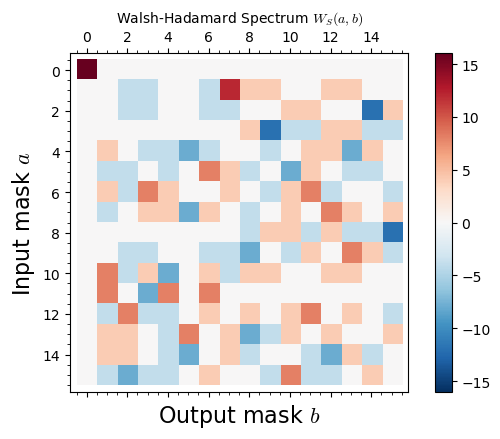
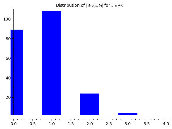
S-box nonlinearity: NL(S) = 2
Maximum Walsh coefficient magnitude (a,b != 0): 12
For a perfect 4-bit S-box, the theoretical maximum nonlinearity is 4.

Experiment 2: Avalanche Effect

The avalanche effect is the most direct manifestation of diffusion. We flip a single bit in the plaintext and measure how many ciphertext bits change. Ideally, flipping one input bit should cause approximately half (8 out of 16) of the output bits to flip.

We measure the avalanche effect as a function of the number of rounds to see how diffusion builds up progressively.

# Avalanche effect experiment (SageMath)

def encrypt_partial(plaintext_bits, round_keys, n_rounds):
    """Encrypt using only the first n_rounds rounds (out of 3+final)."""
    state = list(plaintext_bits)
    
    rounds_done = min(n_rounds, 3)
    for r in range(rounds_done):
        state = ListXOR(state, round_keys[r])
        state = S(state)
        state = P(state)
    
    if n_rounds >= 4:
        state = ListXOR(state, round_keys[2])
        state = S(state)
        state = ListXOR(state, round_keys[3])
    
    return state

# Generate round keys
set_random_seed(2024)
master_key = [choice([0,1]) for _ in range(0, 28)]
round_keys = KeySchedule(master_key)

# Measure avalanche for each round count
n_samples = 2000
max_rounds = 4
avalanche_data = {r: [] for r in range(1, max_rounds + 1)}

for trial in range(n_samples):
    pt = [choice([0,1]) for _ in range(0, 16)]
    flip_bit = ZZ.random_element(0, 16)
    pt_flipped = list(pt)
    pt_flipped[flip_bit] = 1 - pt_flipped[flip_bit]
    
    for nr in range(1, max_rounds + 1):
        ct_orig = encrypt_partial(pt, round_keys, nr)
        ct_flip = encrypt_partial(pt_flipped, round_keys, nr)
        diff = sum(1 for a, b in zip(ct_orig, ct_flip) if a != b)
        avalanche_data[nr].append(diff)

# Plot: mean avalanche per round
means = [mean(avalanche_data[r]) for r in range(1, max_rounds + 1)]
stds = [std(avalanche_data[r]) for r in range(1, max_rounds + 1)]

pts = [(r, float(means[r-1])) for r in range(1, max_rounds + 1)]
p = list_plot(pts, plotjoined=True, marker='o', color='blue',
              legend_label='Measured mean', figsize=7,
              axes_labels=['Number of rounds', 'Mean flipped bits'])
p += line([(0.5, 8), (max_rounds + 0.5, 8)], color='red',
          linestyle='--', legend_label='Ideal (8 bits)')
p.show(ymin=0, ymax=16, title='Avalanche Effect: Convergence to Ideal')

print("\nAvalanche statistics:")
for r in range(1, max_rounds + 1):
    print(f"  Round {r}: mean = {float(means[r-1])):.3f}, std = {float(stds[r-1])):.3f}")
print(f"\nIdeal avalanche: 8.000 bits (half of 16-bit block)")

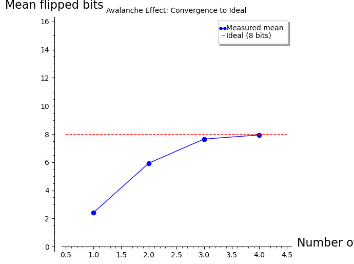
Avalanche statistics:
  Round 1: mean = 2.421, std = 0.550
  Round 2: mean = 5.936, std = 1.693
  Round 3: mean = 7.648, std = 2.188
  Round 4: mean = 7.939, std = 2.105

Ideal avalanche: 8.000 bits (half of 16-bit block)

Experiment 3: Diffusion Heatmap

To visualize diffusion more precisely, we construct a diffusion matrix. For each input bit position \(i\) (0 through 15), we flip that single bit across many random plaintexts and record the probability that each output bit position \(j\) changes. After full diffusion, every entry of this matrix should be close to 0.5.

We show this matrix after each round to observe how diffusion spreads.

# Diffusion heatmap experiment (SageMath)

set_random_seed(2024)
master_key = [choice([0,1]) for _ in range(0, 28)]
round_keys = KeySchedule(master_key)

# Build diffusion matrices for each round
n_samples = 2000
max_rounds = 4
diffusion_matrices = []

for nr in range(1, max_rounds + 1):
    D = matrix(RR, 16, 16, 0)
    for input_bit in range(16):
        for trial in range(n_samples):
            pt = [choice([0,1]) for _ in range(0, 16)]
            pt_flipped = list(pt)
            pt_flipped[input_bit] = 1 - pt_flipped[input_bit]
            ct_orig = encrypt_partial(pt, round_keys, nr)
            ct_flip = encrypt_partial(pt_flipped, round_keys, nr)
            for j in range(16):
                if ct_orig[j] != ct_flip[j]:
                    D[input_bit, j] += 1.0
    D = D / n_samples
    diffusion_matrices.append(D)

# Plot diffusion matrices for all 4 rounds
ga = graphics_array([
    matrix_plot(diffusion_matrices[r], cmap='YlOrRd', vmin=0, vmax=1,
                figsize=4)
    for r in range(4)
], ncols=4)
ga.show(figsize=[20, 5])

print("Mean diffusion probability per round (ideal = 0.500):")
for r in range(4):
    vals = diffusion_matrices[r].list()
    print(f"  Round {r+1}: {float(mean(vals))):.4f}")

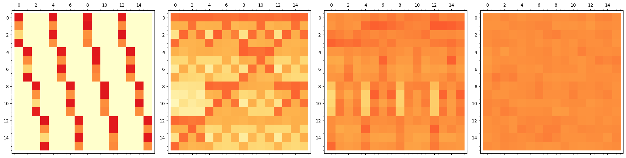
Mean diffusion probability per round (ideal = 0.500):
  Round 1: 0.1524
  Round 2: 0.3718
  Round 3: 0.4816
  Round 4: 0.4949

Experiment 4: Key Schedule Visualization

The key schedule determines which bits of the master key are used in each round. In the Heys tutorial SPN, the key schedule is simple: the 28-bit master key is sliced into four 16-bit windows, each shifted by 4 bits. We visualize which master key bits contribute to each round key.

# Key schedule visualization (SageMath)

n_round_keys = 4
master_key_len = 28
round_key_len = 16

# Build the contribution matrix
contribution = matrix(ZZ, n_round_keys, master_key_len, 0)
for i in range(n_round_keys):
    start = 4 * i
    for j in range(start, start + round_key_len):
        contribution[i, j] = 1

# Plot the key schedule
p = matrix_plot(contribution, cmap='Blues', figsize=10)
p.show(title='Key Schedule: Master Key Bit Usage per Round Key')

print("Key schedule summary:")
for i in range(n_round_keys):
    start = 4 * i
    print(f"  K{i+1}: master key bits [{start}:{start + round_key_len - 1}]")
print(f"\nNote: Each master key bit is used in multiple round keys.")
print(f"Bit overlap between consecutive keys: {round_key_len - 4} bits (out of {round_key_len}).")

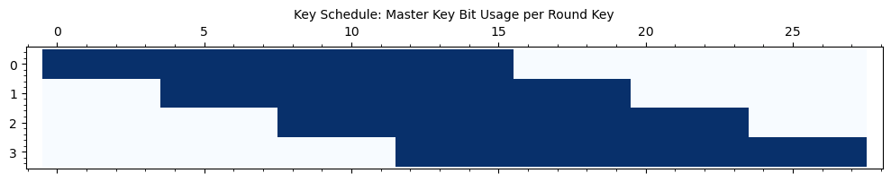
Key schedule summary:
  K1: master key bits [0:15]
  K2: master key bits [4:19]
  K3: master key bits [8:23]
  K4: master key bits [12:27]

Note: Each master key bit is used in multiple round keys.
Bit overlap between consecutive keys: 12 bits (out of 16).

Experiment 5: Comparing S-boxes – Good vs. Poor Design

To appreciate the importance of S-box design, we compare the Heys S-box against two alternatives:

1. The identity S-box (\(S(x) = x\)), which provides no confusion at all.

2. A linear S-box (\(S(x) = Ax\), matrix multiplication over \(\mathrm{GF}(2)\)), which has zero nonlinearity.

We visualize the Walsh spectrum of each to highlight the difference.

# Comparing S-boxes: nonlinear vs linear vs identity (SageMath)

sboxes = {
    'Heys (nonlinear)': [0xE, 0x4, 0xD, 0x1, 0x2, 0xF, 0xB, 0x8,
                         0x3, 0xA, 0x6, 0xC, 0x5, 0x9, 0x0, 0x7],
    'Identity (trivial)': list(range(16)),
    'Linear (affine)': [0x0, 0x5, 0xA, 0xF, 0x3, 0x6, 0x9, 0xC,
                        0x7, 0x2, 0xD, 0x8, 0x4, 0x1, 0xE, 0xB],
}

plots = []
for name, table in sboxes.items():
    W = walsh_hadamard_spectrum(table)
    nl = compute_nonlinearity(W)
    p = matrix_plot(W, cmap='RdBu_r', vmin=-16, vmax=16,
                    figsize=4)
    plots.append(p)

ga = graphics_array(plots, ncols=3)
ga.show(figsize=[18, 5])

print("Nonlinearity comparison:")
for name, table in sboxes.items():
    W = walsh_hadamard_spectrum(table)
    nl = compute_nonlinearity(W)
    max_w = max(abs(w) for w in W[1:, 1:].list())
    print(f"  {name:25s}: NL = {nl}, max|W| = {max_w}")
print("\nThe identity and linear S-boxes have NL = 0, meaning they can be")
print("perfectly approximated by a linear function -- making the cipher")
print("trivially vulnerable to linear cryptanalysis.")

Nonlinearity comparison:
  Heys (nonlinear)         : NL = 2, max|W| = 12
  Identity (trivial)       : NL = 0, max|W| = 16
  Linear (affine)          : NL = 0, max|W| = 16

The identity and linear S-boxes have NL = 0, meaning they can be
perfectly approximated by a linear function -- making the cipher
trivially vulnerable to linear cryptanalysis.

14.7 XOR Encryption and Perfect Secrecy

Before block ciphers, the simplest symmetric encryption is the XOR cipher (one-time pad). Shannon proved in 1949 that the one-time pad achieves perfect secrecy – the ciphertext reveals no information whatsoever about the plaintext – provided the key is at least as long as the message and is used only once.

Theorem 14.1 (Shannon, 1949)

A cryptosystem \((\mathcal{P}, \mathcal{C}, \mathcal{K}, \mathcal{E}, \mathcal{D})\) achieves perfect secrecy if and only if \(|\mathcal{K}| \geq |\mathcal{P}|\), and for every plaintext \(m\) and ciphertext \(c\) with \(\Pr[C = c] > 0\),

\[ \Pr[M = m \mid C = c] = \Pr[M = m].\]

The XOR cipher (one-time pad) with uniformly random keys achieves this bound with equality.

However, perfect secrecy requires keys as long as the message – impractical for most applications. Block ciphers trade perfect secrecy for computational security with short, reusable keys.

# XOR Encryption (One-Time Pad) -- SageMath
# Using SageMath's ^^ for XOR (as in the original course code)

XOR = lambda li1, li2: bytes(a ^^ b for a, b in zip(li1, li2))

def XOREncryption(block, key):
    return XOR(block, key)

def XORDecryption(block, key):
    return XOR(block, key)

# Demonstration
key = b'01101001010101'
plaintext = b'00000000000000'

ciphertext = XOREncryption(plaintext, key)
recovered = XORDecryption(ciphertext, key)

print("XOR Encryption (One-Time Pad) Demonstration")
print("=" * 55)
print(f"Plaintext:  {plaintext}")
print(f"Key:        {key}")
print(f"Ciphertext: {ciphertext}")
print(f"Decrypted:  {recovered}")
print(f"Correct:    {recovered == plaintext}")
print()

# Key reuse vulnerability
print("Key reuse vulnerability:")
msg1 = b'ATTACK AT DAWN'
msg2 = b'DEFEND AT DUSK'
set_random_seed(42)
key_reused = bytes([ZZ.random_element(0, 256) for _ in range(len(msg1))])

c1 = XOREncryption(msg1, key_reused)
c2 = XOREncryption(msg2, key_reused)

# XOR of two ciphertexts = XOR of two plaintexts (key cancels)
c1_xor_c2 = bytes(a ^^ b for a, b in zip(c1, c2))
m1_xor_m2 = bytes(a ^^ b for a, b in zip(msg1, msg2))
print(f"  c1 XOR c2 = {list(c1_xor_c2)}")
print(f"  m1 XOR m2 = {list(m1_xor_m2)}")
print(f"  Equal:      {c1_xor_c2 == m1_xor_m2}")
print("  -> The key cancels! An adversary can recover plaintext XOR differences.")

XOR Encryption (One-Time Pad) Demonstration
=======================================================
Plaintext:  b'00000000000000'
Key:        b'01101001010101'
Ciphertext: b'\x00\x01\x01\x00\x01\x00\x00\x01\x00\x01\x00\x01\x00\x01'
Decrypted:  b'00000000000000'
Correct:    True

Key reuse vulnerability:
  c1 XOR c2 = [5, 17, 18, 4, 13, 15, 0, 0, 0, 0, 0, 20, 4, 5]
  m1 XOR m2 = [5, 17, 18, 4, 13, 15, 0, 0, 0, 0, 0, 20, 4, 5]
  Equal:      True
  -> The key cancels! An adversary can recover plaintext XOR differences.

14.8 Exercises

Exercise 14.1 (S-box Properties). Consider the Heys tutorial S-box \(S = [\text{0xE, 0x4, 0xD, 0x1, 0x2, 0xF, 0xB, 0x8, 0x3, 0xA, 0x6, 0xC, 0x5, 0x9, 0x0, 0x7}]\).

(a) Verify by hand (or by code) that \(S\) is a permutation on \(\{0, 1, \ldots, 15\}\).

(b) Compute the difference distribution table (DDT): for each input difference \(\Delta x \in \{0, \ldots, 15\}\) and output difference \(\Delta y \in \{0, \ldots, 15\}\), count the number of pairs \((x, x')\) with \(x \oplus x' = \Delta x\) and \(S(x) \oplus S(x') = \Delta y\).

(c) What is the maximum value in the DDT (excluding the trivial entry \(\mathrm{DDT}[0][0] = 16\))? This value determines the S-box’s resistance to differential cryptanalysis.

Hint

The DDT can be computed as follows: for each input difference \(\Delta x\) and each input value \(x\), compute \(x' = x \oplus \Delta x\), then \(\Delta y = S(x) \oplus S(x')\). Increment \(\mathrm{DDT}[\Delta x][\Delta y]\). The maximum entry in the Heys S-box DDT (excluding row 0) is 4, which means that for any nonzero input difference, no output difference occurs with probability greater than \(4/16 = 1/4\).

---

Exercise 14.2 (Permutation Layer Design). The Heys permutation \(\pi(i) = 4(i \bmod 4) + \lfloor i/4 \rfloor\) can be viewed as transposing a \(4 \times 4\) matrix of bits.

(a) Write out the full permutation table and verify that \(\pi\) is an involution (i.e., \(\pi(\pi(i)) = i\) for all \(i\)). Use SageMath’s PermutationGroupElement to verify this algebraically.

(b) Explain why this particular permutation achieves good diffusion: after one round, each S-box receives one output bit from each of the four S-boxes of the previous round.

(c) Design an alternative 16-bit permutation that does not achieve good diffusion (e.g., one where the first S-box’s outputs all feed into the same S-box in the next round). Implement it and show that the avalanche effect is significantly worse.

Hint

For part (a), note that transposing a matrix twice returns the original. The Heys permutation maps \(\text{bit } 4i + j \mapsto \text{bit } 4j + i\), which is a matrix transpose. Use Pperm.order() to check that the order is 2 (involution). For part (c), try the identity permutation \(\pi(i) = i\) – this means each S-box feeds only into itself, so there is no cross-S-box diffusion.

---

Exercise 14.3 (Avalanche Criterion). The strict avalanche criterion (SAC) states that flipping any single input bit should cause each output bit to flip with probability exactly \(\frac{1}{2}\).

(a) Does the Heys S-box alone (one application, no key mixing) satisfy the SAC? Test empirically.

(b) Show that after a sufficient number of SPN rounds, the full cipher approximately satisfies the SAC. How many rounds are needed?

(c) Prove that for a random permutation on \(\{0,1\}^n\), the expected number of output bits that change when one input bit is flipped is \(n/2\).

Hint

For part (a), test all 16 inputs: for each input \(x\) and each bit position \(i\), flip bit \(i\) to get \(x' = x \oplus 2^i\), compute \(S(x) \oplus S(x')\), and check whether each output bit flips with probability 1/2 over all choices of \(x\). A 4-bit S-box generally cannot satisfy the SAC perfectly. For part (c), use the fact that for a random permutation, \(S(x)\) and \(S(x')\) are approximately independent, so each output bit has an equal chance of being 0 or 1 in the XOR.

---

Exercise 14.4 (Key Schedule Weakness). The Heys tutorial SPN uses a simple sliding-window key schedule.

(a) How many master key bits does each round key share with its neighbor? What fraction of each round key overlaps with the next?

(b) Argue that this key schedule is weak: if an attacker recovers bits of one round key, they learn bits of neighboring round keys for free.

(c) Design an improved key schedule that uses the S-box to introduce nonlinearity. Describe your design and explain why it would resist the attack in part (b).

Hint

For part (a), consecutive round keys \(K_i\) and \(K_{i+1}\) share 12 out of 16 bits, since \(K_{i+1}\) starts 4 bits later in the master key. This means 75% of each round key is shared with the next. For part (c), consider applying the S-box to parts of each round key and XORing with a round constant (similar to the AES key schedule). This ensures that knowledge of one round key does not directly reveal bits of another.

---

Exercise 14.5 (Full SPN Analysis – Challenge). Implement a function that encrypts all \(2^{16} = 65536\) possible plaintexts under a fixed key using the Heys tutorial SPN.

(a) Verify that the encryption function is indeed a permutation: all 65536 ciphertexts are distinct.

(b) Compute the cycle structure of this permutation using SageMath’s Permutation or PermutationGroupElement. How many cycles are there, and what are their lengths?

(c) Compare the cycle structure to that of a random permutation of 65536 elements. A random permutation of \(N\) elements has approximately \(\ln(N)\) cycles on average. Is the SPN’s cycle structure consistent with a pseudorandom permutation?

Hint

To find cycles, start at element 0, follow \(x \to E_k(x) \to E_k(E_k(x)) \to \cdots\) until you return to 0. Record the cycle length. Then start at the smallest element not yet visited and repeat. In SageMath, you can use Permutation(encryption_list).cycle_type() to get the cycle structure directly. For \(N = 65536\), the expected number of cycles in a random permutation is \(\ln(65536) \approx 11.1\), and the expected length of the longest cycle is approximately \(0.6243 \cdot N \approx 40917\).

14.9 Block Codes with Feistel Structure

One can have an alternative to invertible S-boxes by introducing an architecture which uses non-invertible confusion in a specific way. Such an example was popularized and used widely based on the design described by Horst Feistel.

The Data Encryption Standard (DES) is the most famous example of a Feistel cipher. It operates on 64-bit blocks with a 56-bit key through 16 rounds. The crucial advantage of the Feistel structure is that the round function \(f\) need not be invertible – the structure itself guarantees invertibility:

\[ L_{r+1} = R_r, \qquad R_{r+1} = L_r \oplus f(R_r, K_r).\]

For a complete SageMath implementation of DES, see Chapter 15.

14.10 Summary

In this chapter, we have studied the fundamental design principles underlying modern block ciphers.

Key concepts:

• Confusion (achieved by S-boxes) ensures a complex, nonlinear relationship between the key and the ciphertext. The quality of an S-box is measured by its nonlinearity (via the Walsh-Hadamard transform) and its differential uniformity.

• Diffusion (achieved by P-boxes and linear mixing layers) ensures that each plaintext bit influences many ciphertext bits. The avalanche effect quantifies diffusion: ideally, flipping one input bit causes half the output bits to change.

• The Substitution-Permutation Network (SPN) is a block cipher architecture that alternates S-box substitution with P-box permutation over multiple rounds. Each round also mixes in a round key derived from the master key via a key schedule.

• The Heys tutorial SPN provides a minimal, analyzable example: 16-bit block, 28-bit key, 3 rounds, with a 4-bit S-box and a bit-transposition P-box.

• Perfect secrecy (Shannon, 1949) requires keys as long as the message. Block ciphers sacrifice perfect secrecy for practical key sizes, relying instead on computational security through iterated confusion and diffusion.

SageMath highlights: In this notebook, we used SymmetricGroup and PermutationGroupElement to model the P-box permutation and compute its inverse algebraically, matrix for Walsh-Hadamard spectra, matrix_plot for heatmap visualization, and SageMath’s native ^^ operator for XOR.

Looking ahead. In Chapter 15, we study the DES cipher in detail. In Chapter 16, we use the SPN implemented here as the target for linear cryptanalysis, exploiting linear approximations of the S-box to recover key bits. In Chapter 17, we mount a differential cryptanalysis attack on the same cipher.

Important

The interplay between confusion and diffusion is not merely a design heuristic – it is the reason why modern block ciphers resist the two most powerful generic attacks: linear cryptanalysis and differential cryptanalysis. Understanding this interplay is essential for both designing and breaking block ciphers.

14.11 References

1. Claude E. Shannon, “Communication Theory of Secrecy Systems,” Bell System Technical Journal, 28(4), pp. 656–715, 1949. The foundational paper establishing information-theoretic cryptography. Shannon introduced confusion and diffusion as the two essential properties of a secure cipher and proved that perfect secrecy requires keys at least as long as the message.

2. Howard M. Heys, “A Tutorial on Linear and Differential Cryptanalysis,” Cryptologia, 26(3), pp. 189–221, 2002. An accessible and widely-cited tutorial that introduces a simple SPN cipher (the one implemented in this chapter) and demonstrates linear and differential cryptanalysis on it. The S-box and permutation used here are taken directly from this paper.

3. Horst Feistel, “Cryptography and Computer Privacy,” Scientific American, 228(5), pp. 15–23, May 1973. Feistel’s influential article describing the design principles behind the Lucifer cipher and what later became the DES. This paper introduced the Feistel network structure to the broader scientific community.

4. Horst Feistel, William A. Notz, and J. Lynn Smith, “Some Cryptographic Techniques for Machine-to-Machine Data Communications,” Proceedings of the IEEE, 63(11), pp. 1545–1554, 1975. A more technical treatment of the Feistel cipher design, including discussion of key scheduling and iterative design.

5. Eli Biham and Adi Shamir, “Differential Cryptanalysis of DES-like Cryptosystems,” Journal of Cryptology, 4(1), pp. 3–72, 1991. The paper that introduced differential cryptanalysis, one of the two most important generic attacks on block ciphers. The resistance of an S-box to this attack is measured by its difference distribution table (DDT).

6. Mitsuru Matsui, “Linear Cryptanalysis Method for DES Cipher,” Advances in Cryptology – EUROCRYPT ‘93, LNCS vol. 765, pp. 386–397, Springer, 1994. The paper that introduced linear cryptanalysis. The Walsh-Hadamard spectrum and nonlinearity of the S-box, studied in this chapter, directly determine a cipher’s resistance to this attack.

7. Douglas R. Stinson and Maura B. Paterson, Cryptography: Theory and Practice, 4th edition, CRC Press, 2018. Chapters 4 and 6 provide rigorous treatments of block cipher design, the SPN and Feistel structures, and the mathematical foundations of S-box analysis.