
Chapter 38 — Shor’s Algorithm for Factoring and Discrete Logarithms#
“I think I can safely say that nobody understands quantum mechanics.” — Richard Feynman, 1965
“We show that the problems of prime factorization and discrete logarithms can be solved in polynomial time on a quantum computer.” — Peter Shor, 1994
In this chapter we study Shor’s algorithm, which reduces integer factorization and the discrete logarithm problem to period finding — a task that a quantum computer can solve in polynomial time using the Quantum Fourier Transform. We provide classical simulations for small numbers and examine the profound implications for RSA, Diffie–Hellman, and elliptic-curve cryptography.
38.1 Historical Context#
In 1985, David Deutsch formalized the concept of a quantum Turing machine. Throughout the early 1990s, researchers searched for problems where quantum computers could outperform classical ones beyond artificial oracle problems.
The breakthrough came in 1994 when Peter Shor, then at AT&T Bell Labs, announced a polynomial-time quantum algorithm for integer factorization and the discrete logarithm problem. His paper, published in full in 1997, demonstrated that:
Factoring an \(n\)-bit integer can be done in \(O(n^3 \log n)\) quantum operations (vs. sub-exponential classically).
Discrete logarithms in \(\mathbb{Z}_p^*\) and on elliptic curves can be computed with similar efficiency.
This result sent shockwaves through the cryptographic community because it implies that all widely deployed public-key systems — RSA, Diffie–Hellman, DSA, and ECC — would be broken by a sufficiently large quantum computer.
Key Milestones
Year |
Event |
|---|---|
1985 |
Deutsch defines quantum computation model |
1992 |
Deutsch–Jozsa algorithm: first quantum speedup |
1994 |
Shor announces factoring algorithm at FOCS |
1996 |
Grover’s search algorithm (\(\sqrt{N}\) speedup) |
1997 |
Shor publishes full paper in SIAM J. Computing |
2001 |
IBM factors 15 on a 7-qubit NMR computer |
2019 |
Google claims quantum supremacy (53 qubits) |
2023 |
IBM Condor: 1,121-qubit processor |
2024 |
NIST finalizes post-quantum standards (ML-KEM, ML-DSA) |
38.2 The Core Insight: Factoring as Period Finding#
Shor’s key insight is that factoring reduces to finding the period of a modular exponentiation function, and period finding can be solved efficiently on a quantum computer.
Definition 38.1 — Order (Multiplicative)
For integers \(a\) and \(N\) with \(\gcd(a, N) = 1\), the order of \(a\) modulo \(N\) is the smallest positive integer \(r\) such that
This \(r\) is the period of the function \(f(x) = a^x \bmod N\).
Theorem 38.1 — Reduction of Factoring to Order Finding
Given an odd composite \(N\) and a random \(a\) with \(\gcd(a, N) = 1\):
Find the order \(r\) of \(a\) modulo \(N\).
If \(r\) is even, compute \(x = a^{r/2} \bmod N\).
If \(x \not\equiv -1 \pmod{N}\), then \(\gcd(x \pm 1, N)\) gives nontrivial factors of \(N\).
Proof sketch. If \(r\) is even, then \(a^r - 1 = (a^{r/2} - 1)(a^{r/2} + 1) \equiv 0 \pmod{N}\). Since \(a^{r/2} \not\equiv 1\) (by minimality of \(r\)) and if \(a^{r/2} \not\equiv -1\), then \(N\) divides the product but neither factor individually, so \(\gcd(a^{r/2} \pm 1, N)\) yields a nontrivial factor.
Tip
For a random choice of \(a\), the probability that \(r\) is even and \(a^{r/2} \not\equiv -1\) is at least \(1 - 1/2^{k-1}\), where \(k\) is the number of distinct prime factors of \(N\). For \(N = pq\) (an RSA modulus), this probability is at least \(1/2\).
38.3 The Quantum Fourier Transform#
Definition 38.2 — Quantum Fourier Transform (QFT)
The Quantum Fourier Transform on \(N\) amplitudes maps basis state \(|j\rangle\) to:
where \(\omega = e^{2\pi i / N}\) is a primitive \(N\)-th root of unity.
As a matrix, the QFT is the \(N \times N\) unitary matrix with entries
The QFT is the quantum analogue of the classical Discrete Fourier Transform. The key difference is that a quantum computer can apply the QFT to a superposition of \(N = 2^n\) states using only \(O(n^2)\) gates, whereas the classical FFT requires \(O(N \log N)\) operations on explicit vectors.
Why Period Finding Works
If a quantum register holds a superposition that is periodic with period \(r\), applying the QFT concentrates the amplitudes on multiples of \(N/r\). Measuring one of these peaks and using continued fractions recovers \(r\) exactly.
38.4 Implementation#
We implement a classical simulation of Shor’s algorithm for small numbers. While a real quantum computer would use superposition and entanglement, we can simulate the key mathematical steps — order finding and the QFT — exactly for pedagogical purposes.
import numpy as np
import math
import warnings

def qft_matrix(N):
    """
    Construct the N x N Quantum Fourier Transform matrix.

    F_{jk} = (1/sqrt(N)) * omega^{jk}, where omega = e^{2*pi*i/N}.

    Parameters
    ----------
    N : int
        Dimension of the QFT matrix (typically a power of 2).

    Returns
    -------
    F : ndarray of shape (N, N), complex
        The unitary QFT matrix.
    """
    omega = np.exp(2j * np.pi / N)
    j = np.arange(N)
    k = np.arange(N)
    F = omega ** np.outer(j, k) / np.sqrt(N)
    return F


def abs_det_unitary(M):
    """Compute |det(M)| for a unitary matrix, numerically stable."""
    # For unitary matrices, |det| = 1. We verify via eigenvalues
    # to avoid numerical issues with LU-based det on complex matrices.
    eigs = np.linalg.eigvals(M)
    return float(np.prod(np.abs(eigs)))


# --- Verify unitarity for small sizes ---
for n_qubits in [2, 3, 4]:
    N = 2 ** n_qubits
    F = qft_matrix(N)
    product = F @ F.conj().T
    identity_check = np.allclose(product, np.eye(N), atol=1e-12)
    abs_det = abs_det_unitary(F)
    print(f'QFT({N}x{N}): unitary = {identity_check}, '
          f'|det(QFT)| = {abs_det:.6f}')

# Display the 4x4 QFT matrix
F4 = qft_matrix(4)
print(f'\nQFT matrix for N=4:')
print(f'  (scaled by sqrt(4) = 2 for readability)')
for row in (F4 * 2):
    formatted = [f'{v.real:+.0f}{v.imag:+.0f}j' if abs(v.imag) > 1e-10
                 else f'{v.real:+.0f}' for v in row]
    print(f'  [{"  ".join(formatted)}]')
QFT(4x4): unitary = True, |det(QFT)| = 1.000000
QFT(8x8): unitary = True, |det(QFT)| = 1.000000
QFT(16x16): unitary = True, |det(QFT)| = 1.000000

QFT matrix for N=4:
  (scaled by sqrt(4) = 2 for readability)
  [+1  +1  +1  +1]
  [+1  +0+1j  -1  -0-1j]
  [+1  -1  +1  -1]
  [+1  -0-1j  -1  +0+1j]
import numpy as np
import math

def classical_order_finding(a, N):
    """
    Find the multiplicative order of a modulo N by brute force.

    The order r is the smallest positive integer such that a^r = 1 (mod N).

    Parameters
    ----------
    a : int
        Base, must satisfy gcd(a, N) = 1.
    N : int
        Modulus.

    Returns
    -------
    r : int
        The multiplicative order, or -1 if gcd(a,N) != 1.
    """
    if math.gcd(a, N) != 1:
        return -1
    r = 1
    current = a % N
    while current != 1:
        current = (current * a) % N
        r += 1
        if r > N:
            return -1  # safety check
    return r


def shors_algorithm(N, max_attempts=20, verbose=True):
    """
    Classical simulation of Shor's factoring algorithm.

    Steps:
    1. Check for trivial factors (even, perfect power).
    2. Pick random a in [2, N-1].
    3. Check gcd(a, N) for a lucky factor.
    4. Find the order r of a mod N.
    5. If r is even and a^{r/2} != -1 (mod N), extract factors.

    Parameters
    ----------
    N : int
        Odd composite number to factor.
    max_attempts : int
        Maximum number of random bases to try.
    verbose : bool
        Print intermediate steps.

    Returns
    -------
    factors : tuple of (int, int) or None
        A nontrivial factorization, or None if not found.
    log : list of dict
        Log of each attempt.
    """
    if N % 2 == 0:
        return (2, N // 2), []

    # Check if N is a perfect power
    for b in range(2, int(math.log2(N)) + 1):
        a_root = round(N ** (1.0 / b))
        for candidate in [a_root - 1, a_root, a_root + 1]:
            if candidate > 1 and candidate ** b == N:
                return (candidate, N // candidate), []

    rng = np.random.default_rng(42)
    log = []

    for attempt in range(max_attempts):
        a = int(rng.integers(2, N))
        g = math.gcd(a, N)

        entry = {'attempt': attempt + 1, 'a': a, 'gcd': g}

        if g > 1:
            entry['result'] = 'lucky_gcd'
            entry['factors'] = (g, N // g)
            log.append(entry)
            if verbose:
                print(f'  Attempt {attempt+1}: a={a}, gcd({a},{N})={g} '
                      f'-> lucky factor!')
            return (g, N // g), log

        r = classical_order_finding(a, N)
        entry['order'] = r

        if r % 2 != 0:
            entry['result'] = 'odd_order'
            log.append(entry)
            if verbose:
                print(f'  Attempt {attempt+1}: a={a}, order r={r} (odd, retry)')
            continue

        x = pow(a, r // 2, N)
        entry['a^(r/2) mod N'] = x

        if x == N - 1:  # x = -1 mod N
            entry['result'] = 'minus_one'
            log.append(entry)
            if verbose:
                print(f'  Attempt {attempt+1}: a={a}, r={r}, '
                      f'a^(r/2)={x} = -1 mod {N} (retry)')
            continue

        f1 = math.gcd(x - 1, N)
        f2 = math.gcd(x + 1, N)

        if f1 > 1 and f1 < N:
            entry['result'] = 'success'
            entry['factors'] = (f1, N // f1)
            log.append(entry)
            if verbose:
                print(f'  Attempt {attempt+1}: a={a}, r={r}, '
                      f'a^(r/2)={x}, gcd({x}-1,{N})={f1} -> '
                      f'factors: {f1} x {N//f1}')
            return (f1, N // f1), log
        elif f2 > 1 and f2 < N:
            entry['result'] = 'success'
            entry['factors'] = (f2, N // f2)
            log.append(entry)
            if verbose:
                print(f'  Attempt {attempt+1}: a={a}, r={r}, '
                      f'a^(r/2)={x}, gcd({x}+1,{N})={f2} -> '
                      f'factors: {f2} x {N//f2}')
            return (f2, N // f2), log

        entry['result'] = 'failed'
        log.append(entry)
        if verbose:
            print(f'  Attempt {attempt+1}: a={a}, r={r}, no factor found')

    return None, log


# --- Demo: factor 15 ---
print('Factoring N = 15:')
factors, log = shors_algorithm(15)
if factors:
    print(f'Result: {factors[0]} x {factors[1]} = {factors[0]*factors[1]}')
Factoring N = 15:
  Attempt 1: a=3, gcd(3,15)=3 -> lucky factor!
Result: 3 x 5 = 15
import numpy as np
import math

def simulate_qft_period_finding(a, N, n_qubits=None):
    """
    Simulate the quantum period-finding subroutine classically.

    Constructs the state |x> |a^x mod N> in the first register,
    then applies the QFT to the first register and returns the
    probability distribution over measurement outcomes.

    Parameters
    ----------
    a : int
        Base for modular exponentiation.
    N : int
        Modulus.
    n_qubits : int or None
        Number of qubits in the first register (default: 2*ceil(log2(N))).

    Returns
    -------
    probs : ndarray of shape (Q,)
        Probability of measuring each value in the first register.
    Q : int
        Size of the first register (2^n_qubits).
    r : int
        True period (for reference).
    """
    if n_qubits is None:
        n_qubits = 2 * math.ceil(math.log2(N))
    Q = 2 ** n_qubits

    # Find true order
    r = 1
    val = a % N
    while val != 1:
        val = (val * a) % N
        r += 1

    # Build the state: sum_{x=0}^{Q-1} |x> |a^x mod N>
    # After measuring the second register (or tracing it out),
    # the first register collapses to a uniform superposition
    # over x values with the same a^x mod N value.
    # For simplicity, we pick one residue and keep all x with
    # that residue (equivalent to a particular measurement outcome).

    # Compute a^x mod N for all x
    powers = np.zeros(Q, dtype=int)
    powers[0] = 1
    for x in range(1, Q):
        powers[x] = (powers[x-1] * a) % N

    # Choose the residue a^0 mod N = 1 for definiteness
    # Indices where a^x mod N = 1 are exactly multiples of r
    state = np.zeros(Q, dtype=complex)
    count = 0
    for x in range(Q):
        if powers[x] == 1:
            state[x] = 1.0
            count += 1

    # Normalize
    state /= np.sqrt(count)

    # Apply QFT
    omega = np.exp(2j * np.pi / Q)
    # QFT: out[k] = (1/sqrt(Q)) * sum_x state[x] * omega^{xk}
    qft_state = np.zeros(Q, dtype=complex)
    for k in range(Q):
        qft_state[k] = np.sum(state * omega ** (np.arange(Q) * k)) / np.sqrt(Q)

    probs = np.abs(qft_state) ** 2
    return probs, Q, r


# --- Demo ---
a, N = 7, 15
probs, Q, r = simulate_qft_period_finding(a, N)
print(f'Period finding for a={a}, N={N}')
print(f'Register size Q={Q}, true period r={r}')
print(f'Expected peaks at multiples of Q/r = {Q}/{r} = {float(Q/r):.1f}')
print(f'\nTop measurement outcomes (prob > 0.01):')
for k in range(Q):
    if probs[k] > 0.01:
        print(f'  k={int(k):3d}, prob={float(probs[k]):.4f}, k/Q={float(k/Q):.4f}, '
              f'nearest j/r = {round(k*r/Q)}/{r}')
Period finding for a=7, N=15
Register size Q=256, true period r=4
Expected peaks at multiples of Q/r = 256/4 = 64.0

Top measurement outcomes (prob > 0.01):
  k=  0, prob=0.2500, k/Q=0.0000, nearest j/r = 0/4
  k= 64, prob=0.2500, k/Q=0.2500, nearest j/r = 1/4
  k=128, prob=0.2500, k/Q=0.5000, nearest j/r = 2/4
  k=192, prob=0.2500, k/Q=0.7500, nearest j/r = 3/4
import numpy as np
import math
from fractions import Fraction

def continued_fraction_period(measured_k, Q, N, a=None):
    """
    Extract the period r from a QFT measurement outcome k/Q
    using the continued fraction expansion.

    The continued fraction of k/Q yields a denominator d that may be
    a divisor of the true period r.  To recover r itself, we try
    multiples d, 2d, 3d, ... and (if the base a is provided) verify
    each candidate by checking a^(kd) ≡ 1 (mod N).

    Parameters
    ----------
    measured_k : int
        Measured value from the QFT register.
    Q : int
        Size of the quantum register.
    N : int
        Number being factored (period must be <= N).
    a : int or None
        Base for modular exponentiation.  When provided, candidates
        are verified via a^candidate ≡ 1 (mod N) and the smallest
        verified candidate is placed first.

    Returns
    -------
    r_candidates : list of int
        Candidate periods from convergents of k/Q, with multiples
        appended.  If *a* is given, verified candidates come first.
    """
    if measured_k == 0:
        return []

    frac = Fraction(measured_k, Q).limit_denominator(N)
    d = frac.denominator
    candidates = []

    # The denominator of the best rational approximation
    # to k/Q with denominator <= N is our candidate for r.
    # The true period r may be a multiple of d (when the
    # measurement outcome corresponds to j/r with gcd(j,r) > 1
    # reduced away, or when Q/r is not an integer).
    # Try d, 2d, 3d, ... up to N.
    for mult in range(1, N // d + 1):
        cand = mult * d
        if cand <= N:
            candidates.append(cand)

    # If the base a is known, verify candidates and sort so that
    # the smallest verified period comes first.
    if a is not None and candidates:
        verified = [c for c in candidates if pow(a, c, N) == 1]
        unverified = [c for c in candidates if pow(a, c, N) != 1]
        candidates = verified + unverified

    return candidates


# --- Demo: reconstruct period from measurement ---
a, N = 7, 15
probs, Q, true_r = simulate_qft_period_finding(a, N)

print(f'a={a}, N={N}, Q={Q}, true period r={true_r}')
print(f'\nContinued fraction analysis of peak measurements:')
print(f'{"k":>5} {"k/Q":>10} {"CF denom":>10} {"Best verified":>15} {"Correct?":>10}')

for k in range(Q):
    if probs[k] > 0.01:
        frac = Fraction(k, Q).limit_denominator(N)
        candidates = continued_fraction_period(k, Q, N, a=a)
        correct = true_r in candidates
        best = candidates[0] if candidates else '-'
        print(f'{k:>5} {float(k/Q):>10.4f} {frac.denominator:>10} '
              f'{str(best):>15} {"YES" if correct else "no":>10}')
a=7, N=15, Q=256, true period r=4

Continued fraction analysis of peak measurements:
    k        k/Q   CF denom   Best verified   Correct?
    0     0.0000          1               -         no
   64     0.2500          4               4        YES
  128     0.5000          2               4        YES
  192     0.7500          4               4        YES
How the Classical Simulation Relates to a Real Quantum Computer
Our simulation constructs the full state vector of size \(Q = 2^{2n}\) and applies the QFT as a matrix multiplication. This takes \(O(Q^2)\) classical operations — exponential in \(n\). A real quantum computer applies the QFT in \(O(n^2)\) gates and measures the result probabilistically. The exponential speedup comes from the ability to prepare and manipulate superpositions of \(Q\) states simultaneously.
38.5 Impact on Cryptographic Systems#
Definition 38.3 — Quantum Threat Classification
System |
Hard Problem |
Quantum Attack |
Status |
|---|---|---|---|
RSA |
Integer factoring |
Shor: poly-time |
Broken |
Diffie–Hellman |
Discrete log in \(\mathbb{Z}_p^*\) |
Shor: poly-time |
Broken |
ECDH / ECDSA |
Discrete log on elliptic curves |
Shor variant: poly-time |
Broken |
AES-128 |
Key search (\(2^{128}\)) |
Grover: \(2^{64}\) |
Weakened (double key) |
AES-256 |
Key search (\(2^{256}\)) |
Grover: \(2^{128}\) |
Believed secure |
SHA-256 |
Preimage (\(2^{256}\)) |
Grover: \(2^{128}\) |
Believed secure |
Danger
Shor’s algorithm does not merely weaken RSA or ECC — it breaks them completely. A 4096-bit RSA key, which would take classical computers longer than the age of the universe to factor, could be broken in hours on a sufficiently large quantum computer. The required resources to factor an \(n\)-bit number are roughly \(2n\) logical qubits (Beauregard’s circuit; \({\sim}3n\) in simpler constructions), but with quantum error correction the physical qubit overhead is substantial: Gidney and Ekerå (2021) estimate \({\sim}20\) million noisy physical qubits for RSA-2048 using surface codes.
38.6 Experiments#
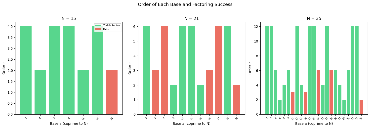
Experiment 1: Factoring N = 15, 21, 35 via Period Finding#
We apply the full Shor reduction for several small semiprimes, showing each step of the algorithm.
Show code cell source
import numpy as np
import math
import matplotlib.pyplot as plt

def order_find(a, N):
    """Find multiplicative order of a mod N."""
    if math.gcd(a, N) != 1:
        return -1
    r, val = 1, a % N
    while val != 1:
        val = (val * a) % N
        r += 1
    return r

targets = [15, 21, 35]

fig, axes = plt.subplots(1, 3, figsize=(15, 5))

for idx, N in enumerate(targets):
    ax = axes[idx]
    print(f'\n{"="*50}')
    print(f'Factoring N = {N}')
    print(f'{"="*50}')

    # Try all bases and collect order data
    bases = []
    orders = []
    success_flags = []

    for a in range(2, N):
        g = math.gcd(a, N)
        if g > 1:
            continue  # skip non-coprime

        r = order_find(a, N)
        bases.append(a)
        orders.append(r)

        success = False
        if r % 2 == 0:
            x = pow(a, r // 2, N)
            if x != N - 1:
                f1 = math.gcd(x - 1, N)
                f2 = math.gcd(x + 1, N)
                if 1 < f1 < N or 1 < f2 < N:
                    success = True
                    factor = f1 if 1 < f1 < N else f2
                    print(f'  a={int(a):2d}: r={r}, a^(r/2)={int(x):2d}, '
                          f'factors: {factor} x {N//factor}')
                else:
                    print(f'  a={int(a):2d}: r={r}, a^(r/2)={int(x):2d}, '
                          f'no nontrivial factor')
            else:
                print(f'  a={int(a):2d}: r={r}, a^(r/2)={int(x):2d} = -1 (mod {N}), fail')
        else:
            print(f'  a={int(a):2d}: r={r} (odd), fail')

        success_flags.append(success)

    n_success = sum(success_flags)
    n_total = len(success_flags)
    print(f'  Success rate: {n_success}/{n_total} = '
          f'{float(n_success/n_total):.1%}')

    # Bar chart of orders
    colors = ['#2ecc71' if s else '#e74c3c' for s in success_flags]
    ax.bar(range(len(bases)), orders, color=colors, alpha=0.8)
    ax.set_xlabel('Base a (coprime to N)')
    ax.set_ylabel('Order r')
    ax.set_title(f'N = {N}')
    ax.set_xticks(range(len(bases)))
    ax.set_xticklabels(bases, fontsize=7, rotation=45)

# Add legend to first axis
from matplotlib.patches import Patch
legend_elements = [Patch(facecolor='#2ecc71', alpha=0.8, label='Yields factor'),
                   Patch(facecolor='#e74c3c', alpha=0.8, label='Fails')]
axes[0].legend(handles=legend_elements, loc='upper right', fontsize=8)

fig.suptitle('Order of Each Base and Factoring Success', fontsize=13, y=1.02)
plt.tight_layout()
plt.savefig('shor_factoring_orders.png', dpi=150, bbox_inches='tight')
plt.show()
==================================================
Factoring N = 15
==================================================
  a= 2: r=4, a^(r/2)= 4, factors: 3 x 5
  a= 4: r=2, a^(r/2)= 4, factors: 3 x 5
  a= 7: r=4, a^(r/2)= 4, factors: 3 x 5
  a= 8: r=4, a^(r/2)= 4, factors: 3 x 5
  a=11: r=2, a^(r/2)=11, factors: 5 x 3
  a=13: r=4, a^(r/2)= 4, factors: 3 x 5
  a=14: r=2, a^(r/2)=14 = -1 (mod 15), fail
  Success rate: 6/7 = 85.7%

==================================================
Factoring N = 21
==================================================
  a= 2: r=6, a^(r/2)= 8, factors: 7 x 3
  a= 4: r=3 (odd), fail
  a= 5: r=6, a^(r/2)=20 = -1 (mod 21), fail
  a= 8: r=2, a^(r/2)= 8, factors: 7 x 3
  a=10: r=6, a^(r/2)=13, factors: 3 x 7
  a=11: r=6, a^(r/2)= 8, factors: 7 x 3
  a=13: r=2, a^(r/2)=13, factors: 3 x 7
  a=16: r=3 (odd), fail
  a=17: r=6, a^(r/2)=20 = -1 (mod 21), fail
  a=19: r=6, a^(r/2)=13, factors: 3 x 7
  a=20: r=2, a^(r/2)=20 = -1 (mod 21), fail
  Success rate: 6/11 = 54.5%

==================================================
Factoring N = 35
==================================================
  a= 2: r=12, a^(r/2)=29, factors: 7 x 5
  a= 3: r=12, a^(r/2)=29, factors: 7 x 5
  a= 4: r=6, a^(r/2)=29, factors: 7 x 5
  a= 6: r=2, a^(r/2)= 6, factors: 5 x 7
  a= 8: r=4, a^(r/2)=29, factors: 7 x 5
  a= 9: r=6, a^(r/2)=29, factors: 7 x 5
  a=11: r=3 (odd), fail
  a=12: r=12, a^(r/2)=29, factors: 7 x 5
  a=13: r=4, a^(r/2)=29, factors: 7 x 5
  a=16: r=3 (odd), fail
  a=17: r=12, a^(r/2)=29, factors: 7 x 5
  a=18: r=12, a^(r/2)=29, factors: 7 x 5
  a=19: r=6, a^(r/2)=34 = -1 (mod 35), fail
  a=22: r=4, a^(r/2)=29, factors: 7 x 5
  a=23: r=12, a^(r/2)=29, factors: 7 x 5
  a=24: r=6, a^(r/2)=34 = -1 (mod 35), fail
  a=26: r=6, a^(r/2)= 6, factors: 5 x 7
  a=27: r=4, a^(r/2)=29, factors: 7 x 5
  a=29: r=2, a^(r/2)=29, factors: 7 x 5
  a=31: r=6, a^(r/2)= 6, factors: 5 x 7
  a=32: r=12, a^(r/2)=29, factors: 7 x 5
  a=33: r=12, a^(r/2)=29, factors: 7 x 5
  a=34: r=2, a^(r/2)=34 = -1 (mod 35), fail
  Success rate: 18/23 = 78.3%
Experiment 2: Visualizing QFT Output Peaks#
We show how the QFT concentrates probability on multiples of \(Q/r\), allowing the period \(r\) to be read from the measurement.
Show code cell source
import numpy as np
import math
import matplotlib.pyplot as plt

def simulate_qft_period(a, N, n_qubits=None):
    """Simulate QFT-based period finding, return probabilities."""
    if n_qubits is None:
        n_qubits = 2 * math.ceil(math.log2(N))
    Q = 2 ** n_qubits

    # Compute order
    r, val = 1, a % N
    while val != 1:
        val = (val * a) % N
        r += 1

    # State after measuring second register as 1
    # -> first register has |0>, |r>, |2r>, ...
    state = np.zeros(Q, dtype=complex)
    count = 0
    for x in range(0, Q, r):
        state[x] = 1.0
        count += 1
    state /= np.sqrt(count)

    # Apply QFT via DFT
    qft_out = np.fft.fft(state, norm='ortho')
    probs = np.abs(qft_out) ** 2
    return probs, Q, r


test_cases = [
    (7, 15, 'a=7, N=15'),
    (2, 21, 'a=2, N=21'),
    (3, 35, 'a=3, N=35'),
    (2, 15, 'a=2, N=15'),
]

fig, axes = plt.subplots(2, 2, figsize=(14, 10))

for ax, (a, N, label) in zip(axes.flat, test_cases):
    probs, Q, r = simulate_qft_period(a, N)

    ax.bar(range(Q), probs, color='#3498db', alpha=0.7, width=1.0)

    # Mark expected peak positions: multiples of Q/r
    for j in range(r):
        peak_pos = j * Q / r
        ax.axvline(x=peak_pos, color='#e74c3c', linestyle='--',
                   alpha=0.6, linewidth=1)

    ax.set_xlabel('Measurement Outcome k')
    ax.set_ylabel('Probability')
    ax.set_title(f'{label}, r={r}, Q={Q}\n'
                 f'Peaks at multiples of Q/r = {float(Q/r):.1f}',
                 fontsize=10)
    ax.set_xlim(-0.5, Q - 0.5)

fig.suptitle('QFT Output: Probability Peaks Reveal the Period',
             fontsize=13, y=1.02)
plt.tight_layout()
plt.savefig('qft_peaks.png', dpi=150, bbox_inches='tight')
plt.show()
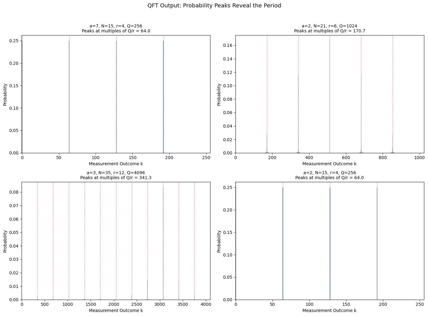
Interpreting the QFT Peaks
Each peak in the QFT output corresponds to a value \(k \approx jQ/r\) for some integer \(j\). There are exactly \(r\) peaks, equally spaced. The spacing \(\Delta k = Q/r\) directly encodes the period \(r\). When \(Q/r\) is not an integer, the peaks broaden slightly, but the continued fraction algorithm can still extract \(r\) with high probability.
Experiment 3: The QFT Matrix Structure#
We visualize the QFT matrix to understand its structure.
Show code cell source
import numpy as np
import matplotlib.pyplot as plt

def qft_matrix(N):
    """Construct N x N QFT matrix."""
    omega = np.exp(2j * np.pi / N)
    j = np.arange(N)
    return omega ** np.outer(j, j) / np.sqrt(N)


fig, axes = plt.subplots(2, 4, figsize=(16, 8))

for i, n_qubits in enumerate([2, 3, 4, 5]):
    N = 2 ** n_qubits
    F = qft_matrix(N)

    # Real part
    ax_re = axes[0, i]
    im_re = ax_re.imshow(F.real, cmap='RdBu', vmin=-0.5, vmax=0.5,
                         aspect='equal', interpolation='nearest')
    ax_re.set_title(f'Re(QFT), {n_qubits} qubits', fontsize=10)
    ax_re.set_xlabel('k')
    ax_re.set_ylabel('j')

    # Imaginary part
    ax_im = axes[1, i]
    im_im = ax_im.imshow(F.imag, cmap='RdBu', vmin=-0.5, vmax=0.5,
                         aspect='equal', interpolation='nearest')
    ax_im.set_title(f'Im(QFT), {n_qubits} qubits', fontsize=10)
    ax_im.set_xlabel('k')
    ax_im.set_ylabel('j')

fig.suptitle('Structure of the Quantum Fourier Transform Matrix',
             fontsize=13, y=1.02)
plt.tight_layout()
plt.savefig('qft_matrix_structure.png', dpi=150, bbox_inches='tight')
plt.show()

# Verify properties using eigenvalue-based |det| (avoids LU overflow)
F8 = qft_matrix(8)
eigs = np.linalg.eigvals(F8)
abs_det = float(np.prod(np.abs(eigs)))
print('Properties of QFT(8):')
print(f'  Unitary: {np.allclose(F8 @ F8.conj().T, np.eye(8))}')
print(f'  Symmetric: {np.allclose(F8, F8.T)}')
print(f'  |det| = {abs_det:.6f}')
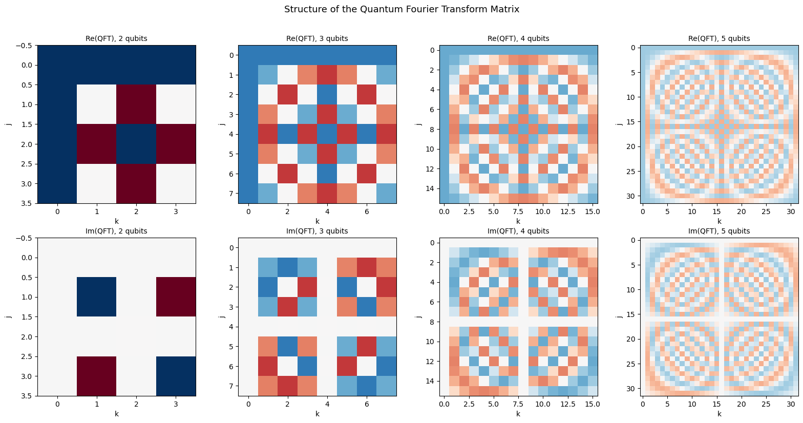
Properties of QFT(8):
  Unitary: True
  Symmetric: True
  |det| = 1.000000
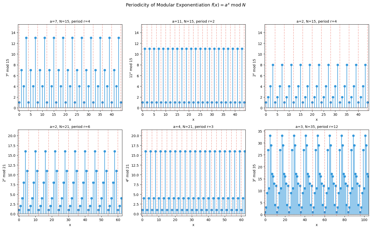
Experiment 4: Modular Exponentiation Periodicity#
We visualize the periodic structure of \(f(x) = a^x \bmod N\) that Shor’s algorithm exploits.
Show code cell source
import numpy as np
import math
import matplotlib.pyplot as plt

fig, axes = plt.subplots(2, 3, figsize=(15, 9))

cases = [
    (7, 15), (11, 15), (2, 15),
    (2, 21), (4, 21), (3, 35),
]

for ax, (a, N) in zip(axes.flat, cases):
    x_vals = np.arange(0, 3 * N)
    y_vals = np.array([pow(a, int(x), N) for x in x_vals])

    # Find order
    r = 1
    val = a % N
    while val != 1 and r < N:
        val = (val * a) % N
        r += 1

    ax.stem(x_vals, y_vals, linefmt='#3498db', markerfmt='o',
            basefmt='gray', label=f'$a^x$ mod {N}')
    ax.set_markersize = 3

    # Mark period boundaries
    for k in range(0, 3 * N, r):
        ax.axvline(x=k, color='#e74c3c', linestyle='--', alpha=0.4)

    ax.set_xlabel('x')
    ax.set_ylabel(f'${a}^x$ mod {N}')
    ax.set_title(f'a={a}, N={N}, period r={r}', fontsize=10)
    ax.set_xlim(-0.5, 3 * N - 0.5)
    ax.set_ylim(-0.5, N + 0.5)

fig.suptitle(r'Periodicity of Modular Exponentiation $f(x) = a^x \;\mathrm{mod}\; N$',
             fontsize=13, y=1.02)
plt.tight_layout()
plt.savefig('modular_exp_periodicity.png', dpi=150, bbox_inches='tight')
plt.show()
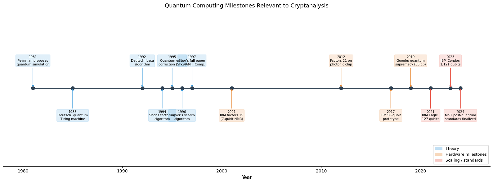
Experiment 5: Timeline of Quantum Computing Milestones#
We visualize the key events in quantum computing relevant to cryptanalysis.
Show code cell source
import numpy as np
import matplotlib.pyplot as plt

milestones = [
    (1981, 'Feynman proposes\nquantum simulation'),
    (1985, 'Deutsch: quantum\nTuring machine'),
    (1992, 'Deutsch-Jozsa\nalgorithm'),
    (1994, 'Shor\'s factoring\nalgorithm'),
    (1995, 'Quantum error\ncorrection (Shor)'),
    (1996, 'Grover\'s search\nalgorithm'),
    (1997, 'Shor\'s full paper\nin SIAM J. Comp.'),
    (2001, 'IBM factors 15\n(7-qubit NMR)'),
    (2012, 'Factors 21 on\nphotonic chip'),
    (2017, 'IBM 50-qubit\nprototype'),
    (2019, 'Google: quantum\nsupremacy (53 qb)'),
    (2021, 'IBM Eagle:\n127 qubits'),
    (2023, 'IBM Condor:\n1,121 qubits'),
    (2024, 'NIST post-quantum\nstandards finalized'),
]

years = [m[0] for m in milestones]
labels = [m[1] for m in milestones]

fig, ax = plt.subplots(figsize=(16, 6))

# Horizontal timeline
ax.plot(years, [0] * len(years), 'o-', color='#2c3e50', markersize=8,
        linewidth=2, zorder=3)

# Alternate labels above and below the timeline
for i, (year, label) in enumerate(milestones):
    direction = 1 if i % 2 == 0 else -1
    offset = 0.35 * direction

    # Color code: theory (blue), hardware (orange), crypto (red)
    if year <= 1997:
        color = '#3498db'  # theory era
    elif year <= 2019:
        color = '#e67e22'  # hardware era
    else:
        color = '#e74c3c'  # quantum advantage era

    ax.annotate(f'{year}\n{label}',
                xy=(year, 0), xytext=(year, offset),
                fontsize=7.5, ha='center', va='center',
                bbox=dict(boxstyle='round,pad=0.3', facecolor=color,
                          alpha=0.15, edgecolor=color),
                arrowprops=dict(arrowstyle='->', color=color, lw=1.2))

ax.set_xlim(1978, 2027)
ax.set_ylim(-1.0, 1.0)
ax.set_xlabel('Year', fontsize=11)
ax.set_title('Quantum Computing Milestones Relevant to Cryptanalysis',
             fontsize=13)
ax.get_yaxis().set_visible(False)
ax.spines['top'].set_visible(False)
ax.spines['left'].set_visible(False)
ax.spines['right'].set_visible(False)

# Legend for color coding
from matplotlib.patches import Patch
legend_elements = [
    Patch(facecolor='#3498db', alpha=0.3, label='Theory'),
    Patch(facecolor='#e67e22', alpha=0.3, label='Hardware milestones'),
    Patch(facecolor='#e74c3c', alpha=0.3, label='Scaling / standards'),
]
ax.legend(handles=legend_elements, loc='lower right', fontsize=9)

plt.tight_layout()
plt.savefig('quantum_timeline.png', dpi=150, bbox_inches='tight')
plt.show()
Experiment 6: Success Probability of Shor’s Algorithm#
We empirically measure the probability that a random base \(a\) yields a factor, and compare it to the theoretical lower bound of \(1/2\) for semiprimes.
Show code cell source
import numpy as np
import math
import matplotlib.pyplot as plt

def shor_success_rate(N):
    """Compute the fraction of bases a that yield a factor of N."""
    successes = 0
    total = 0

    for a in range(2, N):
        if math.gcd(a, N) != 1:
            continue
        total += 1

        # Find order
        r, val = 1, a % N
        while val != 1 and r <= N:
            val = (val * a) % N
            r += 1

        if r % 2 != 0:
            continue
        x = pow(a, r // 2, N)
        if x == N - 1:
            continue
        f1 = math.gcd(x - 1, N)
        f2 = math.gcd(x + 1, N)
        if (1 < f1 < N) or (1 < f2 < N):
            successes += 1

    return successes / total if total > 0 else 0, total


# Semiprimes (products of two distinct primes)
semiprimes = [15, 21, 33, 35, 39, 51, 55, 57, 65, 69, 77, 85,
              87, 91, 93, 95, 111, 115, 119, 123, 129, 133,
              141, 143, 145, 155, 161, 177, 183, 185, 187, 201,
              205, 209, 213, 215, 217, 219, 221]

rates = []
for N in semiprimes:
    rate, total = shor_success_rate(N)
    rates.append(rate)

fig, ax = plt.subplots(figsize=(12, 5))

ax.bar(range(len(semiprimes)), rates, color='#3498db', alpha=0.8)
ax.axhline(y=0.5, color='#e74c3c', linestyle='--', linewidth=2,
           label='Theoretical lower bound (1/2)')
ax.set_xlabel('Semiprime N')
ax.set_ylabel('Success Probability')
ax.set_title('Probability That Random Base Yields Factor (Shor\'s Algorithm)')
ax.set_xticks(range(len(semiprimes)))
ax.set_xticklabels(semiprimes, fontsize=7, rotation=60)
ax.set_ylim(0, 1.05)
ax.legend(fontsize=10)
ax.grid(True, alpha=0.3, axis='y')

mean_rate = np.mean(rates)
ax.axhline(y=mean_rate, color='#2ecc71', linestyle=':',
           linewidth=1.5, label=f'Empirical mean = {float(mean_rate):.2f}')
ax.legend(fontsize=10)

print(f'Mean success rate across {len(semiprimes)} semiprimes: {float(mean_rate):.3f}')
print(f'Min: {float(min(rates)):.3f}, Max: {float(max(rates)):.3f}')

plt.tight_layout()
plt.savefig('shor_success_probability.png', dpi=150, bbox_inches='tight')
plt.show()
Mean success rate across 39 semiprimes: 0.688
Min: 0.503, Max: 0.968
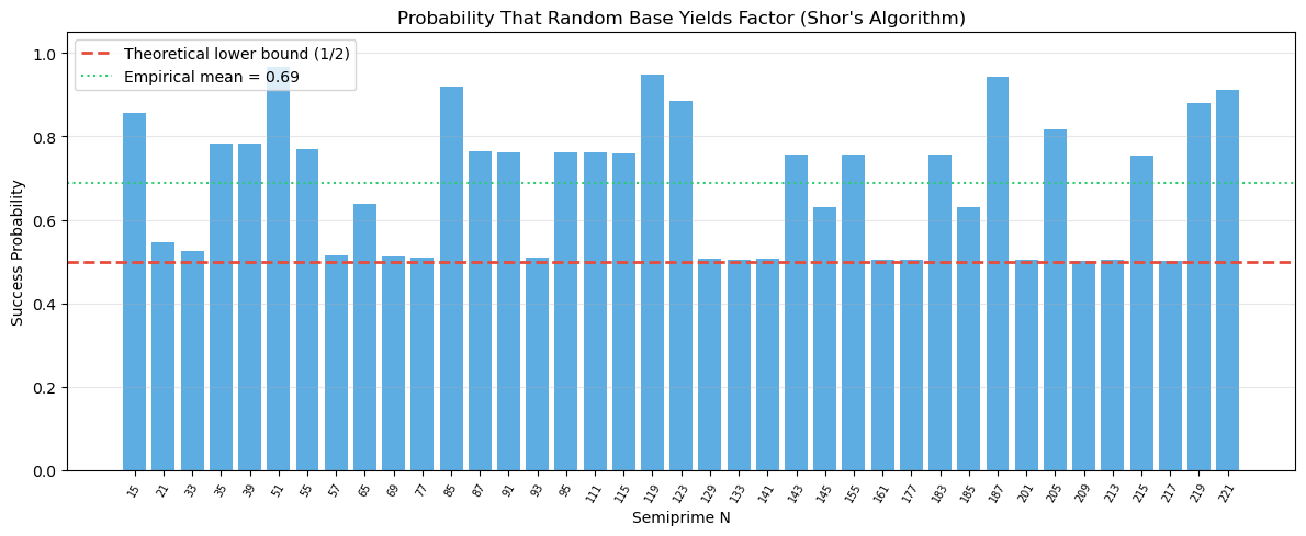
Observation
For semiprimes \(N = pq\), the success probability per attempt is consistently at or above the theoretical lower bound of \(1/2\). Many semiprimes achieve rates of \(3/4\) or higher. This means that, on average, only 1–2 random attempts suffice to factor \(N\), making the algorithm very efficient in expectation.
Experiment 7: Shor’s Algorithm for Discrete Logarithms#
Shor’s algorithm can also solve the discrete logarithm problem: given \(g\), \(h\), and a prime \(p\), find \(x\) such that \(g^x \equiv h \pmod{p}\).
Show code cell source
import numpy as np
import math
import matplotlib.pyplot as plt

def classical_discrete_log(g, h, p):
    """
    Find x such that g^x = h (mod p) by brute force.

    This is the problem that Shor's algorithm solves in polynomial time
    on a quantum computer, breaking Diffie-Hellman and DSA.
    """
    val = 1
    for x in range(p):
        if val == h % p:
            return x
        val = (val * g) % p
    return None


def shor_dlog_reduction(g, h, p):
    """
    Shor's approach to DLP: find the period of f(a,b) = g^a * h^b mod p.

    The function is periodic with period (r, -x*r/ord(g)) where r = ord(g)
    and x = log_g(h). A 2D QFT on the (a,b) register reveals these.

    Here we simulate classically by computing the full 2D function.
    """
    order_g = 1
    val = g % p
    while val != 1:
        val = (val * g) % p
        order_g += 1

    x = classical_discrete_log(g, h, p)

    # Build the 2D function f(a,b) = g^a * h^b mod p
    # for a, b in [0, order_g)
    r = order_g
    func_2d = np.zeros((r, r), dtype=int)
    for a in range(r):
        for b in range(r):
            func_2d[a, b] = (pow(g, a, p) * pow(h, b, p)) % p

    return x, order_g, func_2d


# --- Demo: DLP in small groups ---
test_cases = [
    (2, 8, 13),   # 2^x = 8 mod 13
    (3, 5, 17),   # 3^x = 5 mod 17
    (5, 3, 23),   # 5^x = 3 mod 23
    (2, 11, 29),  # 2^x = 11 mod 29
]

print(f'{"g":>3} {"h":>3} {"p":>4} {"ord(g)":>7} {"x=log_g(h)":>12} '
      f'{"Verify g^x mod p":>17}')
print('=' * 50)

for g, h, p in test_cases:
    x, order_g, _ = shor_dlog_reduction(g, h, p)
    verify = pow(g, x, p)
    print(f'{g:>3} {h:>3} {p:>4} {order_g:>7} {x:>12} {verify:>17}')

# Visualize the 2D periodic function for g=2, h=8, p=13
g, h, p = 2, 8, 13
x, order_g, func_2d = shor_dlog_reduction(g, h, p)

fig, (ax1, ax2) = plt.subplots(1, 2, figsize=(12, 5))

im = ax1.imshow(func_2d, cmap='viridis', aspect='equal', origin='lower')
ax1.set_xlabel('b')
ax1.set_ylabel('a')
ax1.set_title(f'$f(a,b) = {g}^a \\cdot {h}^b$ mod {p}\n'
              f'(x = log_{g}({h}) = {x}, ord({g}) = {order_g})')
plt.colorbar(im, ax=ax1, label='$f(a,b)$ mod p')

# 2D QFT of indicator function for value 1
indicator = (func_2d == 1).astype(float)
qft_2d = np.fft.fft2(indicator)
probs_2d = np.abs(qft_2d) ** 2
probs_2d /= probs_2d.sum()

im2 = ax2.imshow(probs_2d, cmap='hot', aspect='equal', origin='lower')
ax2.set_xlabel('k_b')
ax2.set_ylabel('k_a')
ax2.set_title('2D QFT Probability\n(peaks encode x)')
plt.colorbar(im2, ax=ax2, label='Probability')

plt.tight_layout()
plt.savefig('shor_dlog.png', dpi=150, bbox_inches='tight')
plt.show()
  g   h    p  ord(g)   x=log_g(h)  Verify g^x mod p
==================================================
  2   8   13      12            3                 8
  3   5   17      16            5                 5
  5   3   23      22           16                 3
  2  11   29      28           25                11
Shor’s DLP Algorithm
For the discrete logarithm, Shor uses a two-register approach. The function \(f(a, b) = g^a h^b \bmod p\) has a two-dimensional periodicity structure. A 2D QFT applied to the first two registers reveals lattice points from which the discrete logarithm \(x = \log_g h\) can be extracted using lattice reduction or continued fractions.
The quantum circuit requires \(O(n^2)\) gates for \(n\)-bit primes, giving polynomial-time discrete logarithms. This breaks Diffie-Hellman key exchange, DSA signatures, and all elliptic-curve variants.
Experiment 8: Quantum Resource Estimates#
We estimate the quantum resources (logical qubits, gates) needed to break real-world key sizes, following the analysis of Gidney and Eker\aa{} (2021).
Show code cell source
import numpy as np
import math
import matplotlib.pyplot as plt

# Resource estimates for factoring n-bit RSA moduli
# Sources:
#   - Naive (textbook): ~3n logical qubits (2n for QFT register + n for
#     modular exponentiation workspace) — e.g., Nielsen & Chuang §5.3
#   - Beauregard (2003): ~2n+3 logical qubits using sequential phase
#     estimation and recycling ancillas
#   - Gidney & Ekerå (2021): ~2n + O(1) logical qubits, optimized
#     Toffoli-based modular exponentiation; ~20M noisy physical qubits
#     for RSA-2048 with surface code QEC at ~1500:1 overhead
key_sizes = [512, 1024, 2048, 3072, 4096, 8192]

# Logical qubit estimates
naive_logical = [3 * n for n in key_sizes]           # Textbook: ~3n
beauregard_logical = [2 * n + 3 for n in key_sizes]  # Beauregard: ~2n+3
ge_logical = [2 * n + 300 for n in key_sizes]        # Gidney-Ekerå: ~2n + O(1)

# Gate count: O(n^2 log n) Toffoli gates
toffoli_gates = [n**2 * int(math.log2(n)) for n in key_sizes]

# Physical qubit estimates (surface code QEC overhead)
# Conservative: ~3000 physical per logical (low code distance)
# Optimistic: ~1000 physical per logical (future improvements)
# Gidney-Ekerå target for RSA-2048: ~20M noisy qubits
physical_qubits_conservative = [q * 3000 for q in ge_logical]
physical_qubits_optimistic = [q * 1000 for q in ge_logical]

fig, axes = plt.subplots(1, 3, figsize=(16, 5))

# Logical qubits
ax = axes[0]
ax.semilogy(key_sizes, naive_logical, 'o-', label='Textbook (~3n)',
            color='#e74c3c')
ax.semilogy(key_sizes, beauregard_logical, '^-', label='Beauregard (~2n+3)',
            color='#9b59b6')
ax.semilogy(key_sizes, ge_logical, 's-', label='Gidney-Ekerå (~2n+300)',
            color='#3498db')
ax.set_xlabel('RSA Key Size (bits)')
ax.set_ylabel('Logical Qubits')
ax.set_title('Logical Qubit Requirements')
ax.legend(fontsize=8)
ax.grid(True, alpha=0.3)

# Toffoli gates
ax = axes[1]
ax.semilogy(key_sizes, toffoli_gates, 'o-', color='#e67e22')
ax.set_xlabel('RSA Key Size (bits)')
ax.set_ylabel('Toffoli Gates')
ax.set_title('Gate Count ($O(n^2 \\log n)$)')
ax.grid(True, alpha=0.3)

# Physical qubits
ax = axes[2]
ax.semilogy(key_sizes, physical_qubits_conservative, 'o-',
            label='Conservative (3000:1)', color='#e74c3c')
ax.semilogy(key_sizes, physical_qubits_optimistic, 's-',
            label='Optimistic (1000:1)', color='#2ecc71')
ax.axhline(y=20e6, color='#3498db', linestyle='--', alpha=0.7,
           label='Gidney-Ekerå RSA-2048 target (~20M)')
ax.axhline(y=1121, color='gray', linestyle=':', alpha=0.7,
           label='IBM Condor (1,121 qubits)')
ax.set_xlabel('RSA Key Size (bits)')
ax.set_ylabel('Physical Qubits')
ax.set_title('Physical Qubit Requirements')
ax.legend(fontsize=7)
ax.grid(True, alpha=0.3)

fig.suptitle('Quantum Resources to Break RSA with Shor\'s Algorithm',
             fontsize=13, y=1.02)
plt.tight_layout()
plt.savefig('quantum_resource_estimates.png', dpi=150, bbox_inches='tight')
plt.show()

# Print table
print(f'{"RSA bits":>10} {"Logical (3n)":>13} {"Logical (2n+3)":>15} '
      f'{"Logical (G-E)":>14} {"Phys. (opt)":>13} {"Phys. (cons)":>14}')
print('=' * 82)
for i, n in enumerate(key_sizes):
    print(f'{n:>10} {naive_logical[i]:>13,} {beauregard_logical[i]:>15,} '
          f'{ge_logical[i]:>14,} {physical_qubits_optimistic[i]:>13,} '
          f'{physical_qubits_conservative[i]:>14,}')
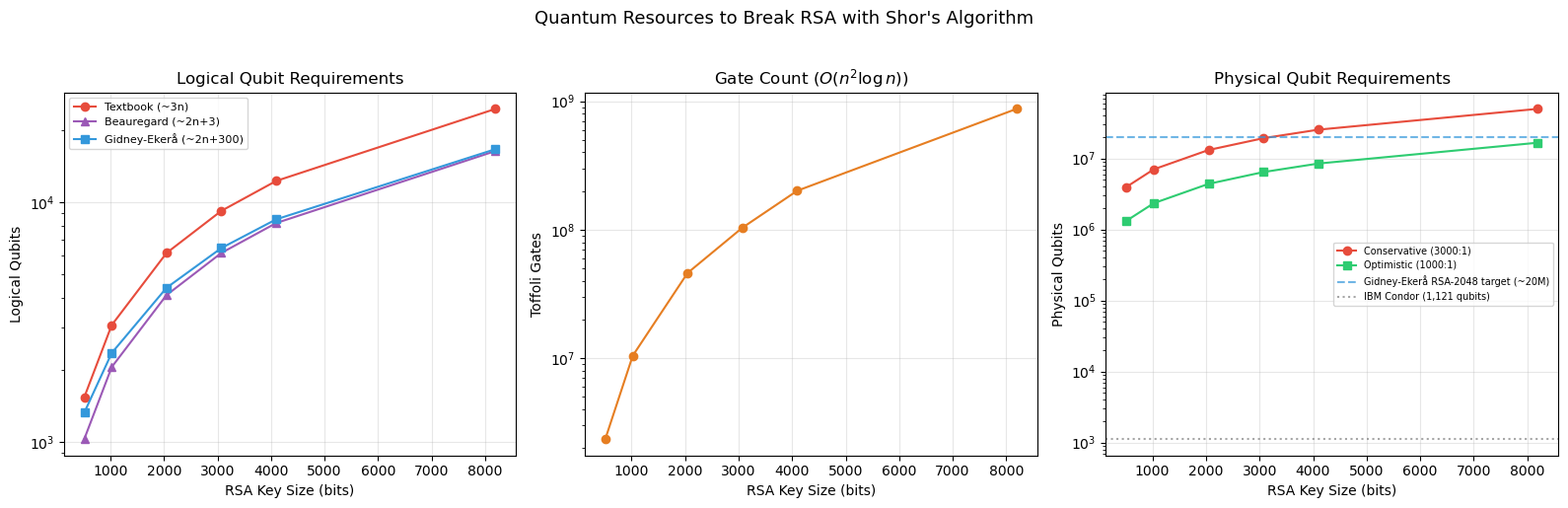
  RSA bits  Logical (3n)  Logical (2n+3)  Logical (G-E)   Phys. (opt)   Phys. (cons)
==================================================================================
       512         1,536           1,027          1,324     1,324,000      3,972,000
      1024         3,072           2,051          2,348     2,348,000      7,044,000
      2048         6,144           4,099          4,396     4,396,000     13,188,000
      3072         9,216           6,147          6,444     6,444,000     19,332,000
      4096        12,288           8,195          8,492     8,492,000     25,476,000
      8192        24,576          16,387         16,684    16,684,000     50,052,000
Danger
The table above shows three logical qubit estimates that reflect different circuit optimizations:
Textbook (\({\sim}3n\)): Uses separate \(2n\)-qubit QFT register and \(n\)-qubit work register — simple but expensive.
Beauregard (\({\sim}2n{+}3\)): Recycles ancillas via sequential phase estimation, nearly halving the logical qubit count.
Gidney–Ekerå (\({\sim}2n{+}300\)): State-of-the-art optimized construction with windowed arithmetic; the additive constant accounts for Toffoli factory workspace.
For RSA-2048 these give roughly 4,000–6,000 logical qubits. The gap to a real machine comes from quantum error correction: with surface codes at a \({\sim}1000\)–\(3000{\times}\) overhead, this translates to 4–13 million physical qubits. Gidney and Ekerå (2021) specifically estimate \({\sim}20\) million noisy physical qubits to factor a 2048-bit RSA integer in 8 hours. As of 2024, the largest quantum processors have around 1,000 physical qubits — orders of magnitude below what is needed.
“Harvest now, decrypt later” attacks make the transition to post-quantum cryptography urgent for long-lived secrets, even though RSA is safe today.
38.7 Exercises#
Exercise 38.1 (Warm-up) For \(N = 21\) and \(a = 2\), compute the order \(r\) of \(a\) modulo \(N\) by hand. Then apply the factoring reduction: is \(r\) even? Does \(a^{r/2} \equiv -1\)? What factors do you obtain?
Hint
Compute: \(2^1 = 2\), \(2^2 = 4\), \(2^3 = 8\), \(2^4 = 16\), \(2^5 = 32 \equiv 11\), \(2^6 = 64 \equiv 1 \pmod{21}\). So \(r = 6\), which is even. \(2^3 = 8\), \(\gcd(7, 21) = 7\), \(\gcd(9, 21) = 3\). Factors: \(3 \times 7\).
Exercise 38.2 (Applied)
Modify the simulate_qft_period_finding function to handle the case where
the second register is measured as a value other than 1. Show that the QFT
peaks are in the same positions regardless of which residue is measured.
Hint
If the second register is measured as \(a^{x_0} \bmod N\), the first register collapses to \(|x_0\rangle + |x_0 + r\rangle + |x_0 + 2r\rangle + \ldots\). The QFT of this shifted periodic signal has the same magnitude spectrum as the unshifted one (by the shift theorem of Fourier analysis).
Exercise 38.3 (Analysis) For \(N = pq\) with \(p, q\) distinct odd primes, prove that the probability of Shor’s algorithm succeeding on a single random \(a\) is at least \(1/2\). What is the probability for \(N = p^2 q\)?
Hint
By CRT, \(\text{ord}_N(a) = \text{lcm}(\text{ord}_p(a), \text{ord}_q(a))\). The algorithm fails only when \(r\) is odd or \(a^{r/2} \equiv -1 \pmod{N}\). Analyze these conditions using the CRT decomposition. For \(N = p^2 q\), there are \(k = 2\) distinct prime factors, so the bound is \(1 - 1/2^{k-1} = 1/2\).
Exercise 38.4 (Theory) Show that the QFT on \(N = 2^n\) states can be implemented with \(n(n-1)/2\) controlled-phase gates and \(n\) Hadamard gates. Write out the circuit for \(n = 3\) qubits.
Hint
The QFT factorizes as a product of operations on individual qubits: \(\text{QFT} = \prod_{j=1}^{n} \left(H_j \prod_{k=j+1}^{n} CR_{k-j}\right)\), followed by a bit-reversal permutation. Each \(CR_m\) is a controlled rotation by \(2\pi / 2^m\). For \(n=3\): \(H_1, CR_1(2\to1), CR_2(3\to1), H_2, CR_1(3\to2), H_3\), then SWAP qubits 1 and 3.
Exercise 38.5 (Challenge) Implement a simulation of Shor’s algorithm that handles composite numbers with more than two prime factors (e.g., \(N = 2 \cdot 3 \cdot 5 = 30\)). Recursively apply the algorithm to fully factor \(N\). Test on \(N \in \{30, 42, 66, 70, 105, 210\}\).
Hint
If Shor’s algorithm returns a factor \(d\) of \(N\), recursively factor both \(d\) and \(N/d\). Use a primality test (trial division is fine for small numbers) to decide when to stop. Handle even numbers and perfect powers as special cases before invoking the period-finding subroutine.
38.8 Summary#
Concept |
Key Point |
|---|---|
Shor’s algorithm (1994) |
Polynomial-time factoring and DLP on a quantum computer |
Core reduction |
Factoring \(\to\) order finding \(\to\) period finding |
Quantum Fourier Transform |
Detects periodicity in superposition; \(O(n^2)\) gates for \(n\) qubits |
Continued fractions |
Extract exact period from QFT measurement outcomes; try multiples of the CF denominator |
Success probability |
\(\geq 1/2\) per attempt for semiprimes \(N = pq\) |
Impact on RSA |
Completely broken; 2048-bit RSA needs ~4,000 logical / ~20M physical qubits |
Impact on DH/ECC |
Completely broken via DLP variant of Shor’s algorithm |
Impact on AES/SHA |
Weakened by Grover (\(\sqrt{}\) speedup), not broken |
Current state |
~1,000 physical qubits; need millions for cryptographic sizes |
Response |
NIST post-quantum standards (ML-KEM, ML-DSA) finalized in 2024 |
Tip
Shor’s algorithm is the primary motivation for the entire field of post-quantum cryptography. In the next chapters, we will examine Grover’s algorithm (Chapter 39) and lattice-based cryptographic constructions (Chapter 40) that resist quantum attacks.
References#
Shor, P. W. (1994). Algorithms for quantum computation: Discrete logarithms and factoring. Proceedings 35th Annual Symposium on Foundations of Computer Science (FOCS), 124–134.
Shor, P. W. (1997). Polynomial-time algorithms for prime factorization and discrete logarithms on a quantum computer. SIAM Journal on Computing, 26(5), 1484–1509.
Nielsen, M. A. and Chuang, I. L. (2010). Quantum Computation and Quantum Information. 10th Anniversary Edition, Cambridge University Press.
Gidney, C. and Eker\aa, M. (2021). How to factor 2048 bit RSA integers in 8 hours using 20 million noisy qubits. Quantum, 5, 433.
NIST (2024). Post-Quantum Cryptography Standardization. FIPS 203 (ML-KEM), FIPS 204 (ML-DSA).
Vandersypen, L. M. K. et al. (2001). Experimental realization of Shor’s quantum factoring algorithm using nuclear magnetic resonance. Nature, 414, 883–887.
Preskill, J. (2018). Quantum computing in the NISQ era and beyond. Quantum, 2, 79.