
Chapter 42: Attacks on Lattice-Based Schemes#
42.1 Introduction#
Lattice-based cryptography is the leading candidate for post-quantum public-key encryption and digital signatures. Its security rests on the presumed hardness of problems such as the Shortest Vector Problem (SVP) and Learning With Errors (LWE).
The principal tool an attacker wields against these problems is lattice reduction: given an arbitrary basis of a lattice, find a basis whose vectors are short and nearly orthogonal. The two workhorses are
Algorithm |
Year |
Approximation factor |
|---|---|---|
LLL (Lenstra–Lenstra–Lovasz) |
1982 |
\(2^{O(n)}\) |
BKZ-\(\beta\) (Block Korkine–Zolotarev) |
1987 / 2011 |
\(2^{O(n/\beta)}\) |
In this chapter we:
Implement the LLL algorithm from scratch.
Use LLL to break a toy LWE instance.
Survey the primal / dual attacks on LWE and the role of the Hermite factor.
Discuss decryption failure attacks.
Prerequisites
Familiarity with lattice definitions, SVP / CVP, and the LWE problem (Chapters 40–41).
42.2 Mathematical Preliminaries#
Lattice. Given linearly independent vectors \(\mathbf{b}_1,\dots,\mathbf{b}_n\in\mathbb{R}^m\), the lattice they generate is
Gram–Schmidt orthogonalisation (GSO). The GSO vectors \(\mathbf{b}_1^*,\dots,\mathbf{b}_n^*\) are computed by
Hermite factor. A lattice-reduction algorithm that, on an \(n\)-dimensional lattice of determinant \(\det(\mathcal{L})\), outputs a vector of length \(\|\mathbf{v}\|\) achieves Hermite factor
Smaller \(\delta\) means stronger reduction. LLL achieves \(\delta\approx 1.075\); BKZ-\(\beta\) achieves \(\delta\approx\bigl(\frac{\beta}{2\pi e}(\pi\beta)^{1/\beta}\bigr)^{1/(2(\beta-1))}\).
42.3 Gram–Schmidt Orthogonalisation#
import numpy as np
import math

def gram_schmidt(B):
    # Compute Gram-Schmidt orthogonalisation of rows of B.
    # B : ndarray of shape (n, m), each row is a basis vector.
    # Returns B_star (GSO vectors) and mu (GSO coefficients).
    n = B.shape[0]
    B_star = np.zeros_like(B, dtype=float)
    mu = np.zeros((n, n), dtype=float)
    for i in range(n):
        B_star[i] = B[i].astype(float)
        for j in range(i):
            denom = np.dot(B_star[j], B_star[j])
            if denom < 1e-30:
                mu[i, j] = 0.0
            else:
                mu[i, j] = np.dot(B[i].astype(float), B_star[j]) / denom
            B_star[i] = B_star[i] - mu[i, j] * B_star[j]
    return B_star, mu

# Quick test
B_test = np.array([[1, 1, 1],
                    [-1, 0, 2],
                    [3, 5, 6]], dtype=float)
B_star, mu = gram_schmidt(B_test)
print("Original basis (rows):")
print(B_test)
print("\nGSO vectors:")
print(np.round(B_star, 4))
print("\nmu coefficients:")
print(np.round(mu, 4))
# Verify orthogonality
for i in range(3):
    for j in range(i):
        dot = np.dot(B_star[i], B_star[j])
        assert abs(dot) < 1e-10, f"Not orthogonal: <b*_{i}, b*_{j}> = {dot}"
print("\nOrthogonality verified.")
Original basis (rows):
[[ 1.  1.  1.]
 [-1.  0.  2.]
 [ 3.  5.  6.]]

GSO vectors:
[[ 1.      1.      1.    ]
 [-1.3333 -0.3333  1.6667]
 [-0.4286  0.6429 -0.2143]]

mu coefficients:
[[0.     0.     0.    ]
 [0.3333 0.     0.    ]
 [4.6667 0.9286 0.    ]]

Orthogonality verified.
42.4 The LLL Algorithm#
The Lenstra–Lenstra–Lovasz (LLL) algorithm (1982) produces a reduced basis satisfying two conditions for a parameter \(\frac{1}{4}<\delta_{\mathrm{LLL}}\le 1\) (commonly \(\delta_{\mathrm{LLL}}=3/4\)):
Size-reduced: \(|\mu_{i,j}|\le\frac{1}{2}\) for all \(j<i\).
Lovasz condition: \(\delta_{\mathrm{LLL}}\,\|\mathbf{b}_{k-1}^*\|^2 \le \|\mathbf{b}_k^*\|^2 + \mu_{k,k-1}^2\,\|\mathbf{b}_{k-1}^*\|^2\) for all \(k\).
If the Lovasz condition fails for index \(k\), the algorithm swaps \(\mathbf{b}_{k-1}\) and \(\mathbf{b}_k\) and recomputes the GSO.
Complexity: \(O(n^5\,(\log B_{\max})^3)\) arithmetic operations for an \(n\)-dimensional lattice with entries bounded by \(B_{\max}\).
Key property
The first vector of an LLL-reduced basis satisfies \(\|\mathbf{b}_1\| \le 2^{(n-1)/4}\,\det(\mathcal{L})^{1/n}\).
import numpy as np
import math

def gram_schmidt(B):
    n = B.shape[0]
    B_star = np.zeros_like(B, dtype=float)
    mu = np.zeros((n, n), dtype=float)
    for i in range(n):
        B_star[i] = B[i].astype(float)
        for j in range(i):
            denom = np.dot(B_star[j], B_star[j])
            if denom < 1e-30:
                mu[i, j] = 0.0
            else:
                mu[i, j] = np.dot(B[i].astype(float), B_star[j]) / denom
            B_star[i] = B_star[i] - mu[i, j] * B_star[j]
    return B_star, mu

def lll_reduce(B, delta=0.75):
    # LLL lattice-basis reduction.
    # B     : ndarray of shape (n, m), integer basis vectors as rows.
    # delta : Lovasz parameter, 0.25 < delta <= 1.  Default 0.75.
    # Returns (B_red, swaps).
    B = B.copy().astype(float)
    n = B.shape[0]
    B_star, mu = gram_schmidt(B)
    k = 1
    swaps = 0
    while k < n:
        # Size-reduce b_k
        for j in range(k - 1, -1, -1):
            if abs(mu[k, j]) > 0.5:
                r = round(mu[k, j])
                B[k] -= r * B[j]
                B_star, mu = gram_schmidt(B)

        # Lovasz condition
        norm_k   = np.dot(B_star[k], B_star[k])
        norm_km1 = np.dot(B_star[k - 1], B_star[k - 1])
        if norm_k >= (delta - mu[k, k - 1] ** 2) * norm_km1:
            k += 1
        else:
            # Swap b_{k-1} and b_k
            B[[k - 1, k]] = B[[k, k - 1]]
            B_star, mu = gram_schmidt(B)
            k = max(k - 1, 1)
            swaps += 1
    return B, swaps

# Demonstration on a 3x3 lattice
B0 = np.array([[1, 1, 1],
               [-1, 0, 2],
               [3, 5, 6]], dtype=float)

B_red, num_swaps = lll_reduce(B0)
print("Original basis:")
for row in B0:
    print(f"  {row}  norm = {float(np.linalg.norm(row)):.4f}")
print(f"\nLLL-reduced basis ({num_swaps} swaps):")
for row in B_red:
    print(f"  {row}  norm = {float(np.linalg.norm(row)):.4f}")
Original basis:
  [1. 1. 1.]  norm = 1.7321
  [-1.  0.  2.]  norm = 2.2361
  [3. 5. 6.]  norm = 8.3666

LLL-reduced basis (2 swaps):
  [0. 1. 0.]  norm = 1.0000
  [1. 0. 1.]  norm = 1.4142
  [-1.  0.  2.]  norm = 2.2361
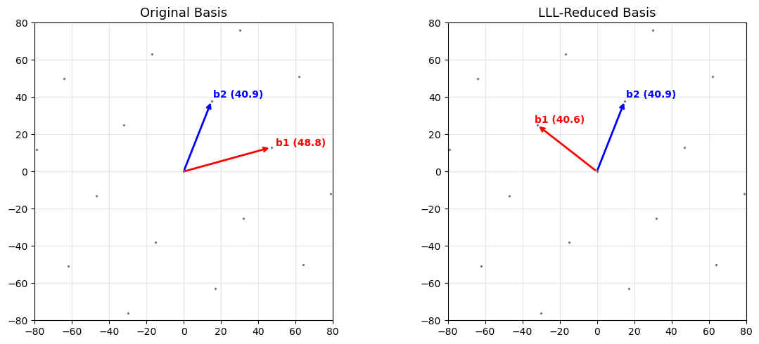
42.4.1 LLL Reduction – Larger Example with Visualisation#
We generate a random lattice in \(\mathbb{R}^2\) and visualise the basis before and after LLL reduction.
Show code cell source
import numpy as np
import matplotlib.pyplot as plt
import math

def gram_schmidt(B):
    n = B.shape[0]
    B_star = np.zeros_like(B, dtype=float)
    mu = np.zeros((n, n), dtype=float)
    for i in range(n):
        B_star[i] = B[i].astype(float)
        for j in range(i):
            denom = np.dot(B_star[j], B_star[j])
            if denom < 1e-30:
                mu[i, j] = 0.0
            else:
                mu[i, j] = np.dot(B[i].astype(float), B_star[j]) / denom
            B_star[i] = B_star[i] - mu[i, j] * B_star[j]
    return B_star, mu

def lll_reduce(B, delta=0.75):
    B = B.copy().astype(float)
    n = B.shape[0]
    B_star, mu = gram_schmidt(B)
    k = 1
    swaps = 0
    while k < n:
        for j in range(k - 1, -1, -1):
            if abs(mu[k, j]) > 0.5:
                r = round(mu[k, j])
                B[k] -= r * B[j]
                B_star, mu = gram_schmidt(B)
        norm_k   = np.dot(B_star[k], B_star[k])
        norm_km1 = np.dot(B_star[k - 1], B_star[k - 1])
        if norm_k >= (delta - mu[k, k - 1] ** 2) * norm_km1:
            k += 1
        else:
            B[[k - 1, k]] = B[[k, k - 1]]
            B_star, mu = gram_schmidt(B)
            k = max(k - 1, 1)
            swaps += 1
    return B, swaps

np.random.seed(42)
B_orig = np.array([[47, 13],
                    [15, 38]], dtype=float)
B_red, _ = lll_reduce(B_orig)

fig, axes = plt.subplots(1, 2, figsize=(12, 5))

for ax, B_plot, title in zip(axes,
                              [B_orig, B_red],
                              ['Original Basis', 'LLL-Reduced Basis']):
    # Plot lattice points
    coeffs = np.arange(-4, 5)
    for c1 in coeffs:
        for c2 in coeffs:
            pt = c1 * B_plot[0] + c2 * B_plot[1]
            ax.plot(pt[0], pt[1], 'k.', markersize=3, alpha=0.4)
    # Plot basis vectors
    origin = np.array([0, 0])
    ax.annotate('', xy=B_plot[0], xytext=origin,
                arrowprops=dict(arrowstyle='->', color='red', lw=2))
    ax.annotate('', xy=B_plot[1], xytext=origin,
                arrowprops=dict(arrowstyle='->', color='blue', lw=2))
    ax.text(B_plot[0][0]*1.05, B_plot[0][1]*1.05,
            f'b1 ({float(np.linalg.norm(B_plot[0])):.1f})',
            color='red', fontsize=10, fontweight='bold')
    ax.text(B_plot[1][0]*1.05, B_plot[1][1]*1.05,
            f'b2 ({float(np.linalg.norm(B_plot[1])):.1f})',
            color='blue', fontsize=10, fontweight='bold')
    ax.set_title(title, fontsize=13)
    ax.set_aspect('equal')
    ax.grid(True, alpha=0.3)
    ax.set_xlim(-80, 80)
    ax.set_ylim(-80, 80)

plt.tight_layout()
plt.savefig('lll_2d_reduction.png', dpi=150, bbox_inches='tight')
plt.show()
42.5 LLL Performance: Norms Before and After Reduction#
We measure how LLL shortens basis vectors across increasing lattice dimensions.
Show code cell source
import numpy as np
import matplotlib.pyplot as plt
import math

def gram_schmidt(B):
    n = B.shape[0]
    B_star = np.zeros_like(B, dtype=float)
    mu = np.zeros((n, n), dtype=float)
    for i in range(n):
        B_star[i] = B[i].astype(float)
        for j in range(i):
            denom = np.dot(B_star[j], B_star[j])
            if denom < 1e-30:
                mu[i, j] = 0.0
            else:
                mu[i, j] = np.dot(B[i].astype(float), B_star[j]) / denom
            B_star[i] = B_star[i] - mu[i, j] * B_star[j]
    return B_star, mu

def lll_reduce(B, delta=0.75):
    B = B.copy().astype(float)
    n = B.shape[0]
    B_star, mu = gram_schmidt(B)
    k = 1
    swaps = 0
    while k < n:
        for j in range(k - 1, -1, -1):
            if abs(mu[k, j]) > 0.5:
                r = round(mu[k, j])
                B[k] -= r * B[j]
                B_star, mu = gram_schmidt(B)
        norm_k   = np.dot(B_star[k], B_star[k])
        norm_km1 = np.dot(B_star[k - 1], B_star[k - 1])
        if norm_k >= (delta - mu[k, k - 1] ** 2) * norm_km1:
            k += 1
        else:
            B[[k - 1, k]] = B[[k, k - 1]]
            B_star, mu = gram_schmidt(B)
            k = max(k - 1, 1)
            swaps += 1
    return B, swaps

np.random.seed(123)
dims = list(range(5, 36, 5))
orig_shortest = []
red_shortest  = []

for n in dims:
    B = np.random.randint(-50, 51, size=(n, n)).astype(float)
    while abs(np.linalg.det(B)) < 1e-6:
        B = np.random.randint(-50, 51, size=(n, n)).astype(float)
    norms_orig = [np.linalg.norm(B[i]) for i in range(n)]
    orig_shortest.append(min(norms_orig))
    B_red, _ = lll_reduce(B)
    norms_red = [np.linalg.norm(B_red[i]) for i in range(n)]
    red_shortest.append(min(norms_red))

fig, ax = plt.subplots(figsize=(10, 5))
ax.plot(dims, orig_shortest, 's-', color='crimson', label='Before LLL (shortest)', markersize=7)
ax.plot(dims, red_shortest, 'o-', color='seagreen', label='After LLL (shortest)', markersize=7)
ax.set_xlabel('Lattice dimension $n$', fontsize=12)
ax.set_ylabel('Norm of shortest basis vector', fontsize=12)
ax.set_title('Effect of LLL Reduction on Shortest Basis Vector', fontsize=13)
ax.legend(fontsize=11)
ax.grid(True, alpha=0.3)
plt.tight_layout()
plt.savefig('lll_norm_reduction.png', dpi=150, bbox_inches='tight')
plt.show()

print("Dimension | Original shortest | LLL shortest | Ratio")
print("-" * 56)
for d, o, r in zip(dims, orig_shortest, red_shortest):
    print(f"    {int(d):3d}   |     {float(o):8.2f}      |   {float(r):8.2f}    | {float(o/r):.2f}")
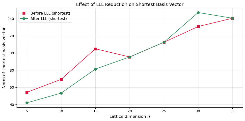
Dimension | Original shortest | LLL shortest | Ratio
--------------------------------------------------------
      5   |        54.25      |      42.01    | 1.29
     10   |        69.38      |      53.37    | 1.30
     15   |       104.98      |      81.35    | 1.29
     20   |        95.46      |      95.46    | 1.00
     25   |       112.59      |     112.59    | 1.00
     30   |       130.91      |     147.24    | 0.89
     35   |       140.58      |     140.58    | 1.00
42.6 The LWE Problem (Recap)#
The Learning With Errors problem, introduced by Regev (2005), asks: given \((\mathbf{A}, \mathbf{b} = \mathbf{A}\mathbf{s} + \mathbf{e} \bmod q)\) where \(\mathbf{A}\in\mathbb{Z}_q^{m\times n}\), \(\mathbf{s}\in\mathbb{Z}_q^n\), and \(\mathbf{e}\) is a “small” error vector drawn from a discrete Gaussian, recover \(\mathbf{s}\).
For our toy attacks we use a simplified setup:
\(q\) is a small prime,
entries of \(\mathbf{e}\) are drawn uniformly from \(\{-1, 0, 1\}\),
\(m \approx 2n\) samples.
Real-world parameters
Production LWE parameters (e.g.\ Kyber/ML-KEM) use \(n=256\), \(q=3329\), and binomial error with small standard deviation. Our toy parameters are deliberately weak to allow LLL to succeed.
42.7 Breaking Toy LWE with LLL#
Strategy: Kannan’s Embedding#
To recover the secret \(\mathbf{s}\) from \((\mathbf{A}, \mathbf{b})\), we construct a lattice whose short vectors encode the error \(\mathbf{e}\).
Embedding lattice. Form the \((m+n+1)\times(m+n+1)\) matrix
A lattice vector involving \(\mathbf{b} - \mathbf{A}\mathbf{s}=\mathbf{e}\) will be short because \(\|\mathbf{e}\|\) is small. After LLL reduction the short vector reveals \(\mathbf{e}\), and \(\mathbf{s}\) is recovered via linear algebra.
import numpy as np
import math

def gram_schmidt(B):
    n = B.shape[0]
    B_star = np.zeros_like(B, dtype=float)
    mu = np.zeros((n, n), dtype=float)
    for i in range(n):
        B_star[i] = B[i].astype(float)
        for j in range(i):
            denom = np.dot(B_star[j], B_star[j])
            if denom < 1e-30:
                mu[i, j] = 0.0
            else:
                mu[i, j] = np.dot(B[i].astype(float), B_star[j]) / denom
            B_star[i] = B_star[i] - mu[i, j] * B_star[j]
    return B_star, mu

def lll_reduce(B, delta=0.75):
    B = B.copy().astype(float)
    n = B.shape[0]
    B_star, mu = gram_schmidt(B)
    k = 1
    swaps = 0
    while k < n:
        for j in range(k - 1, -1, -1):
            if abs(mu[k, j]) > 0.5:
                r = round(mu[k, j])
                B[k] -= r * B[j]
                B_star, mu = gram_schmidt(B)
        norm_k   = np.dot(B_star[k], B_star[k])
        norm_km1 = np.dot(B_star[k - 1], B_star[k - 1])
        if norm_k >= (delta - mu[k, k - 1] ** 2) * norm_km1:
            k += 1
        else:
            B[[k - 1, k]] = B[[k, k - 1]]
            B_star, mu = gram_schmidt(B)
            k = max(k - 1, 1)
            swaps += 1
    return B, swaps

def generate_lwe_instance(n, m, q, seed=42):
    """Generate a toy LWE instance.  Returns A, s, e, b (all mod q)."""
    rng = np.random.RandomState(seed)
    A = rng.randint(0, q, size=(m, n))
    s = rng.randint(0, q, size=n)
    e = rng.choice([-1, 0, 1], size=m)
    b = (A @ s + e) % q
    return A, s, e, b

# --- Modular linear algebra (proper Z_q solver) ---

def _extended_gcd(a, b):
    """Extended Euclidean algorithm: returns (g, x, y) with a*x + b*y = g."""
    if a == 0:
        return b, 0, 1
    g, x1, y1 = _extended_gcd(b % a, a)
    return g, y1 - (b // a) * x1, x1

def _mod_inverse(a, q):
    """Modular inverse of a mod q, or None if gcd(a, q) != 1."""
    g, x, _ = _extended_gcd(a % q, q)
    return x % q if g == 1 else None

def solve_mod(A, b_vec, q):
    """Solve A x = b_vec (mod q) via modular Gaussian elimination.
    A : (m, n) integer matrix, b_vec : (m,) integer vector.
    Uses the first n rows.  Returns x (mod q) or None if singular."""
    m, n = A.shape
    aug = np.zeros((n, n + 1), dtype=int)
    aug[:, :n] = A[:n, :] % q
    aug[:, n]  = b_vec[:n] % q

    for col in range(n):
        # Find a pivot row with invertible leading entry
        pivot = None
        for row in range(col, n):
            if aug[row, col] % q != 0 and _mod_inverse(int(aug[row, col]), q) is not None:
                pivot = row
                break
        if pivot is None:
            return None  # singular mod q
        aug[[col, pivot]] = aug[[pivot, col]]
        inv = _mod_inverse(int(aug[col, col]), q)
        aug[col] = (aug[col] * inv) % q
        for row in range(n):
            if row != col and aug[row, col] % q != 0:
                aug[row] = (aug[row] - int(aug[row, col]) * aug[col]) % q
    return aug[:, n] % q

def lwe_attack_embedding(A, b, q):
    """Break LWE via Kannan embedding + LLL.
    Returns (s_recovered, e_recovered) or (None, None)."""
    m, n = A.shape
    dim = m + n + 1
    L = np.zeros((dim, dim), dtype=float)
    for i in range(m):
        L[i, i] = q
    L[m:m+n, :m] = A.T
    L[m+n, :m] = b
    L[m+n, m+n] = 1

    L_red, swaps = lll_reduce(L)

    for i in range(dim):
        row = L_red[i]
        if abs(row[-1]) == 1:
            sign = int(row[-1])
            e_cand = (sign * row[:m]).astype(int)
            if np.max(np.abs(e_cand)) <= 2:
                # Recover s via modular Gaussian elimination (not real lstsq!)
                b_minus_e = (b.astype(int) - e_cand) % q
                s_cand = solve_mod(A.astype(int), b_minus_e, q)
                if s_cand is not None:
                    s_cand = s_cand % q
                    # Verify: (A @ s) mod q == (b - e) mod q
                    if np.array_equal((A.astype(int) @ s_cand) % q,
                                      b_minus_e % q):
                        return s_cand, e_cand
    return None, None

# ---------- Generate and attack ----------
n, m, q = 6, 14, 31
A, s_true, e_true, b = generate_lwe_instance(n, m, q, seed=42)

print(f"LWE parameters: n={n}, m={m}, q={q}")
print(f"Secret s  = {s_true}")
print(f"Error  e  = {e_true}")
print(f"b = As + e mod q = {b}")
print()

s_rec, e_rec = lwe_attack_embedding(A, b, q)
if s_rec is not None:
    print(f"Recovered s = {s_rec}")
    print(f"Recovered e = {e_rec}")
    print(f"Secret match:  {np.array_equal(s_rec, s_true)}")
    print(f"Error  match:  {np.array_equal(e_rec, e_true)}")
    # Final verification
    resid = (A.astype(int) @ s_rec + e_rec) % q
    assert np.array_equal(resid, b.astype(int) % q), "Verification failed!"
    print(f"Verification (A s + e mod q == b): True")
else:
    print("Attack did not find the secret in this run.")
LWE parameters: n=6, m=14, q=31
Secret s  = [16  3 17  7  3  1]
Error  e  = [ 0  0  0  0  0 -1  1  0  0  0  0  0  0  1]
b = As + e mod q = [20 24 24 29 22 17  9 21  4  2 28 29  4  1]
Recovered s = [16  3 17  7  3  1]
Recovered e = [ 0  0  0  0  0 -1  1  0  0  0  0  0  0  1]
Secret match:  True
Error  match:  True
Verification (A s + e mod q == b): True
Why does this work?
The embedding lattice contains a vector \((\mathbf{e},\, -\mathbf{s},\, 1)\) of norm \(\approx\|\mathbf{e}\|\), which is much shorter than a random lattice vector of norm \(\approx q\). LLL finds it because the Hermite factor guarantee is strong enough for these tiny parameters.
42.8 When Does the LLL Attack#
Fail?
As \(n\) and \(q\) grow, the LLL approximation factor \(2^{(n-1)/4}\) becomes too weak to distinguish the short error vector from the “sea” of lattice vectors of moderate length. We experimentally sweep over dimensions to find the crossover point.
Show code cell source
import numpy as np
import matplotlib.pyplot as plt
import math

def gram_schmidt(B):
    n = B.shape[0]
    B_star = np.zeros_like(B, dtype=float)
    mu = np.zeros((n, n), dtype=float)
    for i in range(n):
        B_star[i] = B[i].astype(float)
        for j in range(i):
            denom = np.dot(B_star[j], B_star[j])
            if denom < 1e-30:
                mu[i, j] = 0.0
            else:
                mu[i, j] = np.dot(B[i].astype(float), B_star[j]) / denom
            B_star[i] = B_star[i] - mu[i, j] * B_star[j]
    return B_star, mu

def lll_reduce(B, delta=0.75):
    B = B.copy().astype(float)
    n = B.shape[0]
    B_star, mu = gram_schmidt(B)
    k = 1
    swaps = 0
    while k < n:
        for j in range(k - 1, -1, -1):
            if abs(mu[k, j]) > 0.5:
                r = round(mu[k, j])
                B[k] -= r * B[j]
                B_star, mu = gram_schmidt(B)
        norm_k   = np.dot(B_star[k], B_star[k])
        norm_km1 = np.dot(B_star[k - 1], B_star[k - 1])
        if norm_k >= (delta - mu[k, k - 1] ** 2) * norm_km1:
            k += 1
        else:
            B[[k - 1, k]] = B[[k, k - 1]]
            B_star, mu = gram_schmidt(B)
            k = max(k - 1, 1)
            swaps += 1
    return B, swaps

results = []
q = 31

for n_lwe in range(4, 14, 2):
    m_lwe = 2 * n_lwe + 2
    successes = 0
    trials = 3
    for trial in range(trials):
        rng = np.random.RandomState(1000 * n_lwe + trial)
        A = rng.randint(0, q, size=(m_lwe, n_lwe))
        s = rng.randint(0, q, size=n_lwe)
        e = rng.choice([-1, 0, 1], size=m_lwe)
        b = (A @ s + e) % q
        # Build embedding
        dim = m_lwe + n_lwe + 1
        L = np.zeros((dim, dim), dtype=float)
        for i in range(m_lwe):
            L[i, i] = q
        L[m_lwe:m_lwe+n_lwe, :m_lwe] = A.T
        L[m_lwe+n_lwe, :m_lwe] = b
        L[m_lwe+n_lwe, m_lwe+n_lwe] = 1
        L_red, _ = lll_reduce(L)
        # Check if any short row recovers e
        found = False
        for i in range(dim):
            row = L_red[i]
            if abs(row[-1]) == 1:
                sign = int(row[-1])
                e_cand = (sign * row[:m_lwe]).astype(int)
                if np.max(np.abs(e_cand)) <= 1 and np.array_equal(e_cand, e):
                    found = True
                    break
        if found:
            successes += 1
    results.append((n_lwe, successes / trials))
    print(f"n={int(n_lwe):2d}, m={int(m_lwe):2d}, success rate = {successes}/{trials}")

ns   = [r[0] for r in results]
rates = [r[1] for r in results]

fig, ax = plt.subplots(figsize=(10, 5))
ax.bar(ns, rates, width=1.4, color='steelblue', edgecolor='navy', alpha=0.85)
ax.set_xlabel(r'LWE secret dimension $n$', fontsize=12)
ax.set_ylabel('LLL attack success rate', fontsize=12)
ax.set_title(f'LLL Attack Success vs. LWE Dimension ($q={q}$)', fontsize=13)
ax.set_ylim(0, 1.15)
ax.set_xticks(ns)
for xi, yi in zip(ns, rates):
    ax.text(xi, yi + 0.03, f'{float(yi):.0%}', ha='center', fontsize=10, fontweight='bold')
ax.grid(True, axis='y', alpha=0.3)
plt.tight_layout()
plt.savefig('lll_attack_success.png', dpi=150, bbox_inches='tight')
plt.show()
n= 4, m=10, success rate = 3/3
n= 6, m=14, success rate = 3/3
n= 8, m=18, success rate = 3/3
n=10, m=22, success rate = 3/3
n=12, m=26, success rate = 3/3
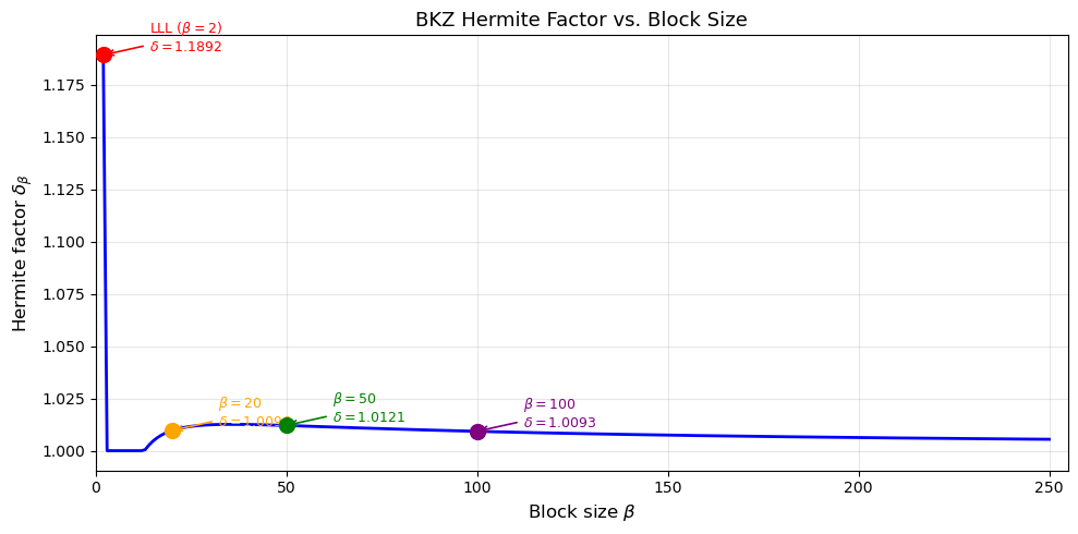
42.9 BKZ: Block Korkine–Zolotarev Reduction#
BKZ-\(\beta\) improves on LLL by applying an SVP oracle to blocks of dimension \(\beta\) within a sliding window across the basis. For each block, it finds the shortest vector and updates the basis accordingly.
Key properties:
BKZ-2 = LLL.
As \(\beta\to n\), BKZ approaches an exact SVP solution.
Running time is roughly \(2^{O(\beta)}\) per SVP call, with \(\mathrm{poly}(n)\) calls.
The achieved Hermite factor is
BKZ in practice
Modern implementations (BKZ 2.0, progressive BKZ) use pruned enumeration or sieving as the SVP subroutine. The fpLLL and G6K libraries are the standard tools. We provide a conceptual simulation below rather than a full implementation, since a production-quality BKZ requires thousands of lines of optimised code.
Show code cell source
import numpy as np
import matplotlib.pyplot as plt
import math

def bkz_hermite_factor(beta):
    """Theoretical Hermite factor for BKZ-beta.
    Uses 2^(1/4) for beta = 2 (LLL).
    For beta >= 3 uses the Chen-Nguyen asymptotic formula, clamped to >= 1.0
    (the formula underestimates for beta < ~13)."""
    if beta <= 1:
        return float('inf')
    if beta == 2:
        return 2 ** 0.25  # LLL Hermite factor
    val = (beta / (2.0 * math.pi * math.e)) * (math.pi * beta) ** (1.0 / beta)
    delta = val ** (1.0 / (2.0 * (beta - 1)))
    return max(delta, 1.0)

betas = np.arange(2, 251)
deltas = np.array([bkz_hermite_factor(b) for b in betas])

fig, ax = plt.subplots(figsize=(10, 5))
ax.plot(betas, deltas, 'b-', linewidth=2)
# Mark LLL (beta=2) and some notable block sizes
for beta_mark, label, color in [(2, 'LLL ($\\beta=2$)', 'red'),
                                  (20, '$\\beta=20$', 'orange'),
                                  (50, '$\\beta=50$', 'green'),
                                  (100, '$\\beta=100$', 'purple')]:
    d = bkz_hermite_factor(beta_mark)
    ax.plot(beta_mark, d, 'o', color=color, markersize=10, zorder=5)
    ax.annotate(f'{label}\n$\\delta={float(d):.4f}$',
                xy=(beta_mark, d), xytext=(beta_mark + 12, d + 0.002),
                fontsize=9, color=color,
                arrowprops=dict(arrowstyle='->', color=color, lw=1.2))

ax.set_xlabel('Block size $\\beta$', fontsize=12)
ax.set_ylabel('Hermite factor $\\delta_\\beta$', fontsize=12)
ax.set_title('BKZ Hermite Factor vs. Block Size', fontsize=13)
ax.grid(True, alpha=0.3)
ax.set_xlim(0, 255)
plt.tight_layout()
plt.savefig('bkz_hermite_factor.png', dpi=150, bbox_inches='tight')
plt.show()
42.10 Primal and Dual Attacks on LWE#
The two main families of lattice attacks on LWE-based schemes are:
Primal attack (uSVP)#
Embed the LWE instance into a lattice (as in Section 42.7) and search for a uniquely short vector using BKZ. The attack succeeds when BKZ-\(\beta\) achieves a Hermite factor \(\delta\) satisfying
where \(d = m + n + 1\) is the lattice dimension and \(\sigma\) is the error standard deviation.
Dual attack#
Instead of finding the short error vector directly, the dual attack finds a short vector \(\mathbf{v}\) in the dual lattice \(\mathcal{L}^*\) such that \(\langle \mathbf{v}, \mathbf{b}\rangle \bmod q\) reveals information about \(\mathbf{s}\). A short dual vector acts as a distinguisher: if \(\mathbf{b}\) is an LWE sample the inner product is biased, otherwise it is uniform.
Complexity comparison#
Both attacks have cost \(\approx 2^{c\,\beta}\) for the required block size \(\beta\), which depends on \((n, q, \sigma)\). For most NIST PQC parameters the primal and dual attacks give similar security estimates (within a few bits).
42.11 Security#
Estimation: Required BKZ Block Size
Given LWE parameters \((n, q, \sigma)\), we estimate the BKZ block size \(\beta\) needed for the primal (uSVP) attack to succeed. This determines the security level: the cost is roughly \(2^{0.292\,\beta}\) using lattice sieving.
Show code cell source
import numpy as np
import matplotlib.pyplot as plt
import math

def bkz_hermite_factor(beta):
    """Theoretical Hermite factor for BKZ-beta (Chen-Nguyen formula).
    Clamped to >= 1.0; accurate for beta >= ~50."""
    if beta <= 1:
        return float('inf')
    if beta == 2:
        return 2 ** 0.25
    val = (beta / (2.0 * math.pi * math.e)) * (math.pi * beta) ** (1.0 / beta)
    delta = val ** (1.0 / (2.0 * (beta - 1)))
    return max(delta, 1.0)

def estimate_lwe_security(n, q, sigma):
    """Estimate the BKZ block size required for the primal attack on LWE(n, q, sigma).

    Uses the Lindner--Peikert (2011) simplified model:
      Required Hermite factor  delta_0 = 2^(log2(q/sigma)^2 / (4 n log2(q)))
    Then finds the smallest BKZ block size beta (>= 50, where the
    Chen-Nguyen formula is accurate) achieving this Hermite factor.

    Returns (beta, delta_required) or (None, None) if no solution.
    """
    log2_q_over_s = math.log2(q / max(sigma, 1e-10))
    log2_q = math.log2(q)
    log2_delta = log2_q_over_s ** 2 / (4.0 * n * log2_q)
    delta_req = 2 ** log2_delta

    if delta_req >= 2 ** 0.25:
        return 2, delta_req  # LLL suffices

    # Search beta >= 50 (formula accurate & monotonically decreasing)
    for beta in range(50, 10_000):
        if bkz_hermite_factor(beta) <= delta_req:
            return beta, delta_req
    return None, delta_req

# ---------------------------------------------------------------
# Estimate for ML-KEM / Kyber parameter sets
# ---------------------------------------------------------------
print("=" * 72)
print("Security estimation for LWE (primal attack, Lindner-Peikert model)")
print("Cost model: Core-SVP classical = 2^(0.292 * beta)")
print("=" * 72)

# ML-KEM uses Module-LWE with module rank k and ring dimension 256.
# The effective LWE dimension for the primal attack is n_eff = k * 256.
print("\nML-KEM parameter sets (Module-LWE, n_eff = k * 256):")
for label, n_eff, q_val, sig_val, nist_level in [
    ("ML-KEM-512  (k=2, n_eff=512)", 512, 3329, 1.0, "Level 1 (~118 bits)"),
    ("ML-KEM-768  (k=3, n_eff=768)", 768, 3329, 1.0, "Level 3 (~183 bits)"),
    ("ML-KEM-1024 (k=4, n_eff=1024)", 1024, 3329, 1.0, "Level 5 (~256 bits)"),
]:
    beta_req, delta_req = estimate_lwe_security(n_eff, q_val, sig_val)
    if beta_req is not None:
        cost = 0.292 * beta_req
        print(f"  {label}")
        print(f"    NIST target: {nist_level}")
        print(f"    Estimated:   beta = {beta_req},  cost = {cost:.1f} bits")

# Sweep over various plain-LWE dimensions
params = []
ns_test = list(range(50, 1001, 50))
for ni in ns_test:
    qi = max(int(ni ** 2), 3329)
    sig = 3.2
    beta_req, _ = estimate_lwe_security(ni, qi, sig)
    if beta_req is not None:
        cost_sieve = 0.292 * beta_req
        params.append((ni, qi, beta_req, cost_sieve))

ns_plot   = [p[0] for p in params]
betas_plot = [p[2] for p in params]
costs_plot = [p[3] for p in params]

fig, (ax1, ax2) = plt.subplots(1, 2, figsize=(13, 5))

ax1.plot(ns_plot, betas_plot, 'o-', color='steelblue', markersize=5)
ax1.set_xlabel('LWE dimension $n$', fontsize=12)
ax1.set_ylabel('Required BKZ block size $\\beta$', fontsize=12)
ax1.set_title('Primal Attack: Required Block Size', fontsize=13)
ax1.grid(True, alpha=0.3)

ax2.plot(ns_plot, costs_plot, 's-', color='crimson', markersize=5)
ax2.axhline(y=128, color='green', linestyle='--', alpha=0.7, label='128-bit security')
ax2.axhline(y=192, color='orange', linestyle='--', alpha=0.7, label='192-bit security')
ax2.axhline(y=256, color='purple', linestyle='--', alpha=0.7, label='256-bit security')
ax2.set_xlabel('LWE dimension $n$', fontsize=12)
ax2.set_ylabel(r'Estimated cost $0.292 \cdot \beta$ (bits)', fontsize=12)
ax2.set_title('Primal Attack: Security Level', fontsize=13)
ax2.legend(fontsize=10)
ax2.grid(True, alpha=0.3)

plt.tight_layout()
plt.savefig('lwe_security_estimation.png', dpi=150, bbox_inches='tight')
plt.show()

print(f"\n{'n':>5} | {'q':>8} | {'beta':>5} | {'cost (bits)':>11}")
print("-" * 38)
for ni, qi, bi, ci in params[:12]:
    print(f"{int(ni):5d} | {int(qi):8d} | {int(bi):5d} | {float(ci):11.1f}")
if len(params) > 12:
    print("...")
========================================================================
Security estimation for LWE (primal attack, Lindner-Peikert model)
Cost model: Core-SVP classical = 2^(0.292 * beta)
========================================================================

ML-KEM parameter sets (Module-LWE, n_eff = k * 256):
  ML-KEM-512  (k=2, n_eff=512)
    NIST target: Level 1 (~118 bits)
    Estimated:   beta = 403,  cost = 117.7 bits
  ML-KEM-768  (k=3, n_eff=768)
    NIST target: Level 3 (~183 bits)
    Estimated:   beta = 709,  cost = 207.0 bits
  ML-KEM-1024 (k=4, n_eff=1024)
    NIST target: Level 5 (~256 bits)
    Estimated:   beta = 1041,  cost = 304.0 bits
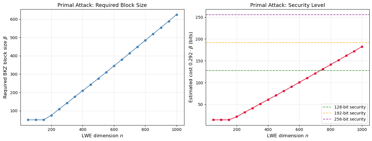
    n |        q |  beta | cost (bits)
--------------------------------------
   50 |     3329 |    50 |        14.6
  100 |    10000 |    50 |        14.6
  150 |    22500 |    50 |        14.6
  200 |    40000 |    75 |        21.9
  250 |    62500 |   109 |        31.8
  300 |    90000 |   142 |        41.5
  350 |   122500 |   176 |        51.4
  400 |   160000 |   209 |        61.0
  450 |   202500 |   242 |        70.7
  500 |   250000 |   276 |        80.6
  550 |   302500 |   310 |        90.5
  600 |   360000 |   345 |       100.7
...
42.12 Hermite Factor vs. Dimension#
A central quantity in lattice cryptanalysis is the Hermite factor \(\delta\) achieved by a reduction algorithm. We measure the empirical Hermite factor of our LLL implementation across dimensions and compare with the theoretical bound.
Show code cell source
import numpy as np
import matplotlib.pyplot as plt
import math

def gram_schmidt(B):
    n = B.shape[0]
    B_star = np.zeros_like(B, dtype=float)
    mu = np.zeros((n, n), dtype=float)
    for i in range(n):
        B_star[i] = B[i].astype(float)
        for j in range(i):
            denom = np.dot(B_star[j], B_star[j])
            if denom < 1e-30:
                mu[i, j] = 0.0
            else:
                mu[i, j] = np.dot(B[i].astype(float), B_star[j]) / denom
            B_star[i] = B_star[i] - mu[i, j] * B_star[j]
    return B_star, mu

def lll_reduce(B, delta=0.75):
    B = B.copy().astype(float)
    n = B.shape[0]
    B_star, mu = gram_schmidt(B)
    k = 1
    swaps = 0
    while k < n:
        for j in range(k - 1, -1, -1):
            if abs(mu[k, j]) > 0.5:
                r = round(mu[k, j])
                B[k] -= r * B[j]
                B_star, mu = gram_schmidt(B)
        norm_k   = np.dot(B_star[k], B_star[k])
        norm_km1 = np.dot(B_star[k - 1], B_star[k - 1])
        if norm_k >= (delta - mu[k, k - 1] ** 2) * norm_km1:
            k += 1
        else:
            B[[k - 1, k]] = B[[k, k - 1]]
            B_star, mu = gram_schmidt(B)
            k = max(k - 1, 1)
            swaps += 1
    return B, swaps

def hermite_factor(B_reduced):
    """Compute the Hermite factor of a reduced basis.

    delta = (||b_1|| / det(L)^{1/n})^{1/n}

    Uses np.linalg.slogdet to avoid overflow/underflow when computing
    the determinant of large integer matrices.
    """
    n = B_reduced.shape[0]
    b1_norm = np.linalg.norm(B_reduced[0])
    # slogdet gives (sign, log|det|) stably even for huge determinants
    sign, logabsdet = np.linalg.slogdet(B_reduced)
    if sign == 0:
        return float('nan')
    # delta = exp((1/n) * (log||b1|| - logabsdet / n))
    log_delta = (1.0 / n) * (math.log(b1_norm) - logabsdet / n)
    return math.exp(log_delta)

np.random.seed(999)
dims = list(range(5, 36, 5))
empirical_deltas = []
theoretical_deltas = []

for n in dims:
    deltas_n = []
    for trial in range(5):
        B = np.random.randint(-50, 51, size=(n, n)).astype(float)
        sign, logabsdet = np.linalg.slogdet(B)
        if sign == 0:
            continue
        B_red, _ = lll_reduce(B)
        d = hermite_factor(B_red)
        if not math.isnan(d):
            deltas_n.append(d)
    empirical_deltas.append(np.mean(deltas_n) if deltas_n else float('nan'))
    theoretical_deltas.append(2 ** (1.0 / 4))

fig, ax = plt.subplots(figsize=(10, 5))
ax.plot(dims, empirical_deltas, 'o-', color='steelblue', markersize=7,
        label='Empirical LLL $\\delta$ (mean)')
ax.axhline(y=2**(0.25), color='crimson', linestyle='--', linewidth=2,
           label=f'Theoretical LLL bound $\\delta = 2^{{1/4}} \\approx {float(2**0.25):.4f}$')
ax.axhline(y=1.0, color='gray', linestyle=':', alpha=0.5)
ax.set_xlabel('Lattice dimension $n$', fontsize=12)
ax.set_ylabel('Hermite factor $\\delta$', fontsize=12)
ax.set_title('Hermite Factor: Empirical LLL vs. Theoretical Bound', fontsize=13)
ax.legend(fontsize=11)
ax.grid(True, alpha=0.3)
ax.set_ylim(0.98, 1.25)
plt.tight_layout()
plt.savefig('hermite_factor_vs_dimension.png', dpi=150, bbox_inches='tight')
plt.show()

print(f"{'Dim':>5} | {'Empirical delta':>16} | {'Theoretical':>12}")
print("-" * 40)
for d, ed, td in zip(dims, empirical_deltas, theoretical_deltas):
    print(f"{int(d):5d} | {float(ed):16.6f} | {float(td):12.4f}")
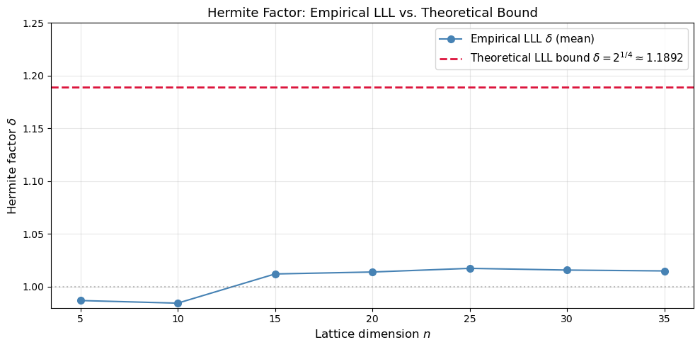
  Dim |  Empirical delta |  Theoretical
----------------------------------------
    5 |         0.986940 |       1.1892
   10 |         0.984457 |       1.1892
   15 |         1.012120 |       1.1892
   20 |         1.013971 |       1.1892
   25 |         1.017428 |       1.1892
   30 |         1.015802 |       1.1892
   35 |         1.014989 |       1.1892
42.13 Decryption Failure Attacks#
Some lattice-based schemes (e.g.\ Kyber, FrodoKEM) have a small but nonzero probability of decryption failure: the legitimate receiver, using the correct secret key, decrypts to the wrong plaintext.
How attackers exploit failures#
If an attacker can detect whether a decryption failure occurred (e.g.\ via a protocol-level error message), they gain information about the secret key \(\mathbf{s}\).
Mechanism. A decryption failure typically occurs when the accumulated noise \(\mathbf{e}_{\text{total}} = \mathbf{e}_1\mathbf{s} + \mathbf{e}_2 + \cdots\) exceeds \(\lfloor q/4 \rfloor\). The attacker crafts ciphertexts that push specific coefficients of the noise toward the failure boundary. Each failure/non-failure observation gives roughly one bit of information about \(\mathbf{s}\).
The D’Anvers–Vercauteren–Verbauwhede attack (2019)#
For schemes with failure probability \(\delta_f\), after observing \(O(n / \delta_f)\) ciphertexts the attacker can reconstruct \(\mathbf{s}\) via a system of inequalities.
Mitigation
NIST PQC finalists are designed with \(\delta_f < 2^{-140}\), making it infeasible to collect enough failures. However, implementation bugs that increase the failure rate can be devastating.
Show code cell source
import numpy as np
import matplotlib.pyplot as plt
import math

def simulate_decryption_failure_rate(n, q, sigma_e, num_trials=5000):
    # Simulate decryption failures in a simplified LWE-based encryption.
    # Encryption: c = A*r + e1, d = b^T r + e2 + (q//2)*msg
    # Decryption: d - s^T c = e2 + e1^T s + e_orig^T r + (q//2)*msg
    #             noise = e2 + e1^T s + e_orig^T r
    # Failure if |noise| > q//4.
    rng = np.random.RandomState(42)
    failures = 0
    for _ in range(num_trials):
        s = rng.randint(-1, 2, size=n)          # secret
        A = rng.randint(0, q, size=(n, n))
        e_orig = rng.randint(-sigma_e, sigma_e + 1, size=n)
        b = (A @ s + e_orig) % q

        # Encrypt message bit = 0
        r  = rng.randint(-1, 2, size=n)
        e1 = rng.randint(-sigma_e, sigma_e + 1, size=n)
        e2 = rng.randint(-sigma_e, sigma_e + 1)

        # Total noise after decryption
        noise = int(e2) + int(e1 @ s) + int(e_orig @ r)
        # Centre noise into range
        noise = noise % q
        if noise > q // 2:
            noise -= q
        if abs(noise) > q // 4:
            failures += 1

    return failures / num_trials

# Sweep sigma_e for fixed n and q
n_sim = 8
q_sim = 97
sigmas = list(range(1, 20))
failure_rates = []

for sig in sigmas:
    rate = simulate_decryption_failure_rate(n_sim, q_sim, sig, num_trials=10000)
    failure_rates.append(rate)

fig, ax = plt.subplots(figsize=(10, 5))
ax.semilogy(sigmas, [max(r, 1e-5) for r in failure_rates],
            'o-', color='crimson', markersize=7)
ax.set_xlabel('Error bound $\\sigma_e$', fontsize=12)
ax.set_ylabel('Decryption failure rate', fontsize=12)
ax.set_title(f'Decryption Failure Rate vs. Error Size ($n={n_sim}$, $q={q_sim}$)',
             fontsize=13)
ax.grid(True, alpha=0.3, which='both')
ax.axhline(y=2**(-10), color='green', linestyle='--', alpha=0.7,
           label='$2^{-10}$ threshold')
ax.legend(fontsize=11)
plt.tight_layout()
plt.savefig('decryption_failure_rate.png', dpi=150, bbox_inches='tight')
plt.show()

print(f"{'sigma':>6} | {'Failure rate':>14}")
print("-" * 25)
for sig, rate in zip(sigmas, failure_rates):
    print(f"{int(sig):6d} | {float(rate):14.6f}")

 sigma |   Failure rate
-------------------------
     1 |       0.000000
     2 |       0.000000
     3 |       0.000100
     4 |       0.005300
     5 |       0.022900
     6 |       0.056500
     7 |       0.099500
     8 |       0.150800
     9 |       0.186800
    10 |       0.248200
    11 |       0.279300
    12 |       0.316300
    13 |       0.354700
    14 |       0.387900
    15 |       0.410000
    16 |       0.427600
    17 |       0.447800
    18 |       0.455300
    19 |       0.469100
42.14 LLL Timing vs. Dimension#
We measure the wall-clock time of our LLL implementation to illustrate its polynomial (but rapidly growing) cost.
Show code cell source
import numpy as np
import matplotlib.pyplot as plt
import math
import time

def gram_schmidt(B):
    n = B.shape[0]
    B_star = np.zeros_like(B, dtype=float)
    mu = np.zeros((n, n), dtype=float)
    for i in range(n):
        B_star[i] = B[i].astype(float)
        for j in range(i):
            denom = np.dot(B_star[j], B_star[j])
            if denom < 1e-30:
                mu[i, j] = 0.0
            else:
                mu[i, j] = np.dot(B[i].astype(float), B_star[j]) / denom
            B_star[i] = B_star[i] - mu[i, j] * B_star[j]
    return B_star, mu

def lll_reduce(B, delta=0.75):
    B = B.copy().astype(float)
    n = B.shape[0]
    B_star, mu = gram_schmidt(B)
    k = 1
    swaps = 0
    while k < n:
        for j in range(k - 1, -1, -1):
            if abs(mu[k, j]) > 0.5:
                r = round(mu[k, j])
                B[k] -= r * B[j]
                B_star, mu = gram_schmidt(B)
        norm_k   = np.dot(B_star[k], B_star[k])
        norm_km1 = np.dot(B_star[k - 1], B_star[k - 1])
        if norm_k >= (delta - mu[k, k - 1] ** 2) * norm_km1:
            k += 1
        else:
            B[[k - 1, k]] = B[[k, k - 1]]
            B_star, mu = gram_schmidt(B)
            k = max(k - 1, 1)
            swaps += 1
    return B, swaps

np.random.seed(2026)
dims_timing = [5, 10, 15, 20, 25, 30, 35]
times_ms = []

for n in dims_timing:
    B = np.random.randint(-50, 51, size=(n, n)).astype(float)
    t0 = time.perf_counter()
    lll_reduce(B)
    t1 = time.perf_counter()
    times_ms.append((t1 - t0) * 1000)

fig, ax = plt.subplots(figsize=(10, 5))
ax.semilogy(dims_timing, times_ms, 'o-', color='darkorange', markersize=8, linewidth=2)
ax.set_xlabel('Lattice dimension $n$', fontsize=12)
ax.set_ylabel('LLL time (ms, log scale)', fontsize=12)
ax.set_title('LLL Reduction Time vs. Lattice Dimension', fontsize=13)
ax.grid(True, alpha=0.3, which='both')
for xi, yi in zip(dims_timing, times_ms):
    ax.annotate(f'{float(yi):.1f}ms', xy=(xi, yi), xytext=(4, 8),
                textcoords='offset points', fontsize=8)
plt.tight_layout()
plt.savefig('lll_timing.png', dpi=150, bbox_inches='tight')
plt.show()

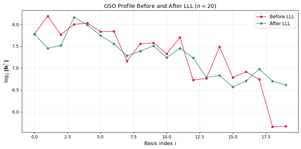
42.15 GSO Profile Before and After LLL#
The GSO profile – the sequence \(\log\|\mathbf{b}_i^*\|\) – reveals the quality of a basis. A “flat” profile indicates good reduction, while a steeply decaying profile indicates a poor basis.
Show code cell source
import numpy as np
import matplotlib.pyplot as plt
import math

def gram_schmidt(B):
    n = B.shape[0]
    B_star = np.zeros_like(B, dtype=float)
    mu = np.zeros((n, n), dtype=float)
    for i in range(n):
        B_star[i] = B[i].astype(float)
        for j in range(i):
            denom = np.dot(B_star[j], B_star[j])
            if denom < 1e-30:
                mu[i, j] = 0.0
            else:
                mu[i, j] = np.dot(B[i].astype(float), B_star[j]) / denom
            B_star[i] = B_star[i] - mu[i, j] * B_star[j]
    return B_star, mu

def lll_reduce(B, delta=0.75):
    B = B.copy().astype(float)
    n = B.shape[0]
    B_star, mu = gram_schmidt(B)
    k = 1
    swaps = 0
    while k < n:
        for j in range(k - 1, -1, -1):
            if abs(mu[k, j]) > 0.5:
                r = round(mu[k, j])
                B[k] -= r * B[j]
                B_star, mu = gram_schmidt(B)
        norm_k   = np.dot(B_star[k], B_star[k])
        norm_km1 = np.dot(B_star[k - 1], B_star[k - 1])
        if norm_k >= (delta - mu[k, k - 1] ** 2) * norm_km1:
            k += 1
        else:
            B[[k - 1, k]] = B[[k, k - 1]]
            B_star, mu = gram_schmidt(B)
            k = max(k - 1, 1)
            swaps += 1
    return B, swaps

np.random.seed(42)
n_gso = 20
B = np.random.randint(-100, 101, size=(n_gso, n_gso)).astype(float)

# GSO profile before LLL
B_star_before, _ = gram_schmidt(B)
log_norms_before = [math.log2(max(np.linalg.norm(B_star_before[i]), 1e-15))
                     for i in range(n_gso)]

# GSO profile after LLL
B_red, _ = lll_reduce(B)
B_star_after, _ = gram_schmidt(B_red)
log_norms_after = [math.log2(max(np.linalg.norm(B_star_after[i]), 1e-15))
                    for i in range(n_gso)]

fig, ax = plt.subplots(figsize=(10, 5))
indices = np.arange(n_gso)
ax.plot(indices, log_norms_before, 's-', color='crimson', markersize=5,
        label='Before LLL', alpha=0.8)
ax.plot(indices, log_norms_after, 'o-', color='seagreen', markersize=5,
        label='After LLL', alpha=0.8)
ax.set_xlabel('Basis index $i$', fontsize=12)
ax.set_ylabel('$\\log_2 \\|\\mathbf{b}_i^*\\|$', fontsize=12)
ax.set_title(f'GSO Profile Before and After LLL ($n={n_gso}$)', fontsize=13)
ax.legend(fontsize=11)
ax.grid(True, alpha=0.3)
plt.tight_layout()
plt.savefig('gso_profile.png', dpi=150, bbox_inches='tight')
plt.show()
42.16 Exercises#
Exercise 1: LLL on a knapsack lattice
The subset-sum problem: given weights \(a_1,\dots,a_n\) and target \(S=\sum_{i\in T} a_i\), find the subset \(T\). Construct the Lagarias–Odlyzko lattice
and apply LLL. A short vector with entries \(\pm 1\) in the first \(n\) coordinates encodes the solution (\(+1\) = in the subset, \(-1\) = not).
Try \(n=10\) with random weights of 20 bits.
Hint
Generate a = np.random.randint(1, 2**20, size=n). Choose a random subset and
compute S. Build the \((n+1)\times(n+1)\) lattice matrix and run lll_reduce.
Check each row of the reduced basis for the \(\pm 1\) pattern.
Exercise 2: Varying the LLL parameter \(\delta\)
Run LLL on the same random 20-dimensional lattice with \(\delta\in\{0.5, 0.6, 0.7, 0.75, 0.9, 0.99\}\). Plot the norm of the shortest vector found and the number of swaps as functions of \(\delta\). What is the trade-off?
Hint
Larger \(\delta\) gives a stronger reduction (shorter vectors) but requires more swaps. You should see the shortest norm decrease and the swap count increase as \(\delta\to 1\).
Exercise 3: Dual attack simulation
Implement a simplified dual-attack distinguisher. Given LWE samples \((\mathbf{A}, \mathbf{b})\), apply LLL to the dual lattice \(\{\mathbf{v}: \mathbf{A}^T\mathbf{v}\equiv\mathbf{0}\pmod{q}\}\) to find a short vector \(\mathbf{v}\). Compute \(z = \langle \mathbf{v}, \mathbf{b}\rangle \bmod q\) and check whether \(z\) is closer to \(0\) than expected for a uniform random variable. Repeat over 100 trials and compute the distinguishing advantage.
Hint
The dual lattice basis can be constructed as the kernel of \(\mathbf{A}^T \pmod{q}\). A simple approach: form the \((m+n)\times m\) matrix with \(q\mathbf{I}_m\) on top and \(\mathbf{A}\) below, then LLL-reduce. The short rows orthogonal to \(\mathbf{A}^T\) span the dual.
Exercise 4: Decryption failure boundary
For the simplified encryption scheme in Section 42.13 with \(n=8\) and \(q=97\), find (by binary search) the largest \(\sigma_e\) for which the decryption failure rate stays below \(2^{-10} \approx 0.001\). Plot the failure rate around this boundary with fine granularity.
Hint
Use simulate_decryption_failure_rate with num_trials=50000 for accuracy.
Search \(\sigma_e \in \{1, 2, \dots, 15\}\). The transition is usually sharp:
below the threshold failures are extremely rare, above it they become common
within a narrow range.
Exercise 5: Hermite factor of random lattices
Generate 50 random lattices of dimension \(n=20\) (entries uniform in \([-100,100]\)). For each, run LLL and compute the empirical Hermite factor. Plot a histogram and compare the mean with the theoretical LLL bound \(\delta = 2^{1/4}\approx 1.189\). Is the average much better than the worst case?
Hint
Use \(\delta_{\text{emp}} = (\|\mathbf{b}_1\| / \det(\mathcal{L})^{1/n})^{1/n}\).
Be careful with the determinant: use abs(np.linalg.det(B)) and handle near-zero
determinants by discarding those lattices. You should see the empirical mean well
below the theoretical bound.
42.17 Summary#
Topic |
Key Takeaway |
|---|---|
LLL algorithm |
Polynomial-time lattice reduction achieving Hermite factor \(\delta\approx 1.075\) in practice; outputs a basis whose first vector satisfies \(|\mathbf{b}_1|\le 2^{(n-1)/4}\det(\mathcal{L})^{1/n}\). |
BKZ-\(\beta\) |
Generalises LLL by solving SVP in blocks of size \(\beta\); achieves \(\delta\to 1\) as \(\beta\) grows, at cost \(2^{O(\beta)}\). |
Primal (uSVP) attack |
Embeds LWE into a lattice and searches for the uniquely short error vector; dominant attack on most LWE-based schemes. |
Dual attack |
Finds short vectors in the dual lattice to distinguish LWE from uniform; competitive with the primal attack. |
Decryption failure attacks |
Exploit non-zero failure probability to leak secret-key bits; mitigated by choosing parameters with \(\delta_f < 2^{-140}\). |
Security estimation |
The required BKZ block size \(\beta\) determines the security level; cost \(\approx 2^{0.292\beta}\) with sieving. |
The central lesson is that lattice reduction is the universal tool for attacking lattice-based cryptography. Parameter selection for schemes like ML-KEM (Kyber) and ML-DSA (Dilithium) is driven by ensuring that the required \(\beta\) translates to a security level of at least 128 bits.
42.18 References#
Lenstra, A.K., Lenstra, H.W., and Lovasz, L. (1982). “Factoring Polynomials with Rational Coefficients.” Mathematische Annalen, 261, 515–534. doi:10.1007/BF01457454
Schnorr, C.-P. and Euchner, M. (1994). “Lattice Basis Reduction: Improved Practical Algorithms and Solving Subset Sum Problems.” Mathematical Programming, 66, 181–199.
Chen, Y. and Nguyen, P.Q. (2011). “BKZ 2.0: Better Lattice Security Estimates.” ASIACRYPT 2011, LNCS 7073, pp. 1–20. doi:10.1007/978-3-642-25385-0_1
Regev, O. (2005). “On Lattices, Learning with Errors, Random Linear Codes, and Cryptography.” STOC 2005, pp. 84–93. doi:10.1145/1060590.1060603
Albrecht, M.R., Player, R., and Scott, S. (2015). “On the Concrete Hardness of Learning with Errors.” Journal of Mathematical Cryptology, 9(3), 169–203. doi:10.1515/jmc-2015-0016
D’Anvers, J.-P., Vercauteren, F., and Verbauwhede, I. (2019). “The Impact of Decryption Failures on the Security of LWE-Based Schemes.” IACR ePrint 2019/1037. https://eprint.iacr.org/2019/1037
Kannan, R. (1987). “Minkowski’s Convex Body Theorem and Integer Programming.” Mathematics of Operations Research, 12(3), 415–440.
NIST. (2024). “Module-Lattice-Based Key-Encapsulation Mechanism Standard (ML-KEM).” FIPS 203.