
Chapter 17: Linear Approximation Tables and Trail Construction#
17.1 Historical Context: Matsui’s Systematic Approach#
In 1993, Mitsuru Matsui published a landmark paper that changed the landscape of block cipher cryptanalysis. His technique, linear cryptanalysis, exploited statistical linear relationships between plaintext bits, ciphertext bits, and key bits to mount a known-plaintext attack on the full 16-round DES. Matsui’s approach required \(2^{43}\) known plaintext-ciphertext pairs – a number that was practically achievable – and represented the first publicly demonstrated attack faster than brute force against DES.
The key innovation was systematic trail construction. Rather than searching randomly for useful linear approximations, Matsui developed an algorithmic method to trace linear trails through the cipher’s structure. Each trail passes through a sequence of S-boxes, accumulating bias at every step according to the piling-up lemma (Chapter 16). The art of linear cryptanalysis lies in finding trails with the largest cumulative bias – these are the trails that require the fewest known plaintexts to exploit.
In 1994, Kaisa Nyberg introduced the concept of linear hulls, which formalized the observation that many distinct linear trails can connect the same input and output masks. The total bias of a linear approximation is not determined by any single trail but by the sum over all trails connecting those masks. This insight revealed that Matsui’s single-trail analysis could both overestimate and underestimate the true bias, depending on whether the contributing trails interfere constructively or destructively.
“The linear hull effect shows that the security of a cipher against linear cryptanalysis cannot be evaluated by considering only the best linear trail.”
– Kaisa Nyberg, “Linear Approximation of Block Ciphers” (1994)
Important
Linear trails vs. linear hulls. A linear trail specifies the exact sequence of intermediate masks through every round of the cipher. A linear hull aggregates all trails that share the same input and output masks. The distinction is analogous to the difference between a single differential characteristic and a differential in differential cryptanalysis.
17.2 Formal Definitions#
We now formalize the notion of a linear trail through a Substitution-Permutation Network (SPN). Throughout this section, we work with the Heys tutorial SPN: a 16-bit block cipher with four 4-bit S-boxes per round.
Definition 17.1 (Linear Trail through an SPN)
Let \(\mathcal{C}\) be an \(r\)-round SPN with \(n\)-bit block size, \(m\) S-boxes of \(s\) bits each per round, and a bit permutation \(\pi\) between rounds. A linear trail \(\mathcal{T}\) is a sequence of input masks:
where \(\alpha_0 \in \{0,1\}^n\) is the plaintext mask, \(\alpha_r \in \{0,1\}^n\) is the mask after the final round’s S-box layer, and for each intermediate round \(i\) (\(1 \leq i \leq r-1\)), the mask \(\alpha_i\) satisfies:
The output mask of S-box \(j\) in round \(i\) is the subset of bits of \(\alpha_i\) corresponding to S-box \(j\).
The input mask of each S-box in round \(i+1\) is obtained by applying the bit permutation \(\pi\) to \(\alpha_i\).
The trail is valid if every active S-box has a non-zero bias for its (input mask, output mask) pair.
Definition 17.2 (Active S-box in a Linear Trail)
An S-box in round \(i\) of a linear trail \(\mathcal{T}\) is called active if the input mask to that S-box is non-zero. Equivalently, S-box \(j\) in round \(i\) is active if at least one of the \(s\) bits in the corresponding portion of the round’s input mask is 1.
The total number of active S-boxes in a trail is denoted \(a(\mathcal{T})\). A trail with fewer active S-boxes generally has a higher bias and is therefore more useful for the attack.
Definition 17.3 (Trail Bias via the Piling-Up Lemma)
Let \(\mathcal{T}\) be a linear trail with \(a\) active S-boxes, and let \(\varepsilon_1, \varepsilon_2, \ldots, \varepsilon_a\) be the biases of the linear approximations used at each active S-box. By the piling-up lemma, the bias of the entire trail is:
where each \(\varepsilon_i = \frac{N_i}{2^s} - \frac{1}{2}\), with \(N_i\) the number of inputs \(x\) satisfying the linear approximation \(\alpha_i \cdot x \oplus \beta_i \cdot S(x) = 0\) for the \(i\)-th active S-box.
Theorem 17.1 (Composite Trail Bias)
For a linear trail \(\mathcal{T}\) through \(r\) rounds of an SPN with \(a = a(\mathcal{T})\) active S-boxes and individual S-box biases \(\varepsilon_1, \ldots, \varepsilon_a\), the overall trail bias is:
This follows from iterated application of the piling-up lemma under the assumption that the round keys are independent and uniformly distributed (the independent-key assumption).
Proof
The piling-up lemma states that if \(X_1, X_2, \ldots, X_a\) are independent binary random variables with biases \(\varepsilon_1, \ldots, \varepsilon_a\) respectively (i.e., \(\Pr[X_i = 0] = \frac{1}{2} + \varepsilon_i\)), then the XOR \(X_1 \oplus X_2 \oplus \cdots \oplus X_a\) has bias:
Under the independent-key assumption, the linear approximation at each active S-box behaves as an independent binary random variable. The overall trail approximation is the XOR of all individual approximations, so the piling-up lemma applies directly. \(\square\)
17.3 Computing the Linear Approximation Table#
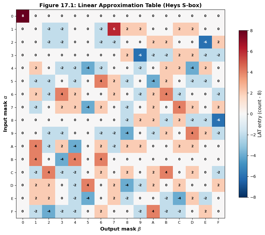
Before we can find linear trails, we need the Linear Approximation Table (LAT) of the S-box, which records the bias of every possible (input mask, output mask) pair. We computed the LAT in Chapter 16; here we reproduce the computation and extract the bias values needed for trail analysis.
import numpy as np
import matplotlib.pyplot as plt

# Heys tutorial S-box (4-bit)
SBOX = np.array([0xE, 0x4, 0xD, 0x1, 0x2, 0xF, 0xB, 0x8,
                 0x3, 0xA, 0x6, 0xC, 0x5, 0x9, 0x0, 0x7], dtype=np.int32)

# Bit permutation (16-bit, 0-indexed)
PERM = np.array([0, 4, 8, 12, 1, 5, 9, 13, 2, 6, 10, 14, 3, 7, 11, 15], dtype=np.int32)

def compute_lat(sbox):
    """
    Compute the Linear Approximation Table for a given S-box.

    Returns the LAT as a 2D array where LAT[a][b] = count of x
    satisfying (a . x) XOR (b . S(x)) = 0, minus 2^(n-1).
    """
    n = len(sbox)
    bits = int(np.log2(n))
    lat = np.zeros((n, n), dtype=np.int32)

    for input_mask in range(n):
        for output_mask in range(n):
            count = 0
            for x in range(n):
                # Compute parity of (input_mask AND x) XOR (output_mask AND S(x))
                input_parity = bin(input_mask & x).count('1') % 2
                output_parity = bin(output_mask & sbox[x]).count('1') % 2
                if input_parity == output_parity:
                    count += 1
            lat[input_mask][output_mask] = count - n // 2

    return lat

lat = compute_lat(SBOX)
print("Linear Approximation Table (LAT) for Heys S-box")
print("=" * 70)
print(f"{'':>4s}", end="")
for b in range(16):
    print(f"{b:>4x}", end="")
print()
print("-" * 70)
for a in range(16):
    print(f"{a:>3x}|", end="")
    for b in range(16):
        print(f"{int(lat[a][b]):>4d}", end="")
    print()

print(f"\nMax absolute bias entry (excluding [0][0]): {np.max(np.abs(lat[1:, 1:]))}")
print(f"This corresponds to a probability bias of {np.max(np.abs(lat[1:, 1:]))}/16 = {float(np.max(np.abs(lat[1:, 1:])) / 16):.4f}")
Linear Approximation Table (LAT) for Heys S-box
======================================================================
       0   1   2   3   4   5   6   7   8   9   a   b   c   d   e   f
----------------------------------------------------------------------
  0|   8   0   0   0   0   0   0   0   0   0   0   0   0   0   0   0
  1|   0   0  -2  -2   0   0  -2   6   2   2   0   0   2   2   0   0
  2|   0   0  -2  -2   0   0  -2  -2   0   0   2   2   0   0  -6   2
  3|   0   0   0   0   0   0   0   0   2  -6  -2  -2   2   2  -2  -2
  4|   0   2   0  -2  -2  -4  -2   0   0  -2   0   2   2  -4   2   0
  5|   0  -2  -2   0  -2   0   4   2  -2   0  -4   2   0  -2  -2   0
  6|   0   2  -2   4   2   0   0   2   0  -2   2   4  -2   0   0  -2
  7|   0  -2   0   2   2  -4   2   0  -2   0   2   0   4   2   0   2
  8|   0   0   0   0   0   0   0   0  -2   2   2  -2   2  -2  -2  -6
  9|   0   0  -2  -2   0   0  -2  -2  -4   0  -2   2   0   4   2  -2
  a|   0   4  -2   2  -4   0   2  -2   2   2   0   0   2   2   0   0
  b|   0   4   0  -4   4   0   4   0   0   0   0   0   0   0   0   0
  c|   0  -2   4  -2  -2   0   2   0   2   0   2   4   0   2   0  -2
  d|   0   2   2   0  -2   4   0   2  -4  -2   2   0   2   0   0   2
  e|   0   2   2   0  -2  -4   0   2  -2   0   0  -2  -4   2  -2   0
  f|   0  -2  -4  -2  -2   0   2   0   0  -2   4  -2  -2   0   2   0

Max absolute bias entry (excluding [0][0]): 6
This corresponds to a probability bias of 6/16 = 0.3750
Show code cell source
import numpy as np
import matplotlib.pyplot as plt

SBOX = np.array([0xE, 0x4, 0xD, 0x1, 0x2, 0xF, 0xB, 0x8,
                 0x3, 0xA, 0x6, 0xC, 0x5, 0x9, 0x0, 0x7], dtype=np.int32)

def compute_lat(sbox):
    n = len(sbox)
    lat = np.zeros((n, n), dtype=np.int32)
    for input_mask in range(n):
        for output_mask in range(n):
            count = 0
            for x in range(n):
                ip = bin(input_mask & x).count('1') % 2
                op = bin(output_mask & sbox[x]).count('1') % 2
                if ip == op:
                    count += 1
            lat[input_mask][output_mask] = count - n // 2
    return lat

lat = compute_lat(SBOX)

fig, ax = plt.subplots(figsize=(10, 8))
im = ax.imshow(lat, cmap='RdBu_r', vmin=-8, vmax=8, aspect='equal')
ax.set_xticks(range(16))
ax.set_yticks(range(16))
ax.set_xticklabels([f'{i:X}' for i in range(16)], fontsize=9)
ax.set_yticklabels([f'{i:X}' for i in range(16)], fontsize=9)
ax.set_xlabel('Output mask $\\beta$', fontsize=12, fontweight='bold')
ax.set_ylabel('Input mask $\\alpha$', fontsize=12, fontweight='bold')
ax.set_title('Figure 17.1: Linear Approximation Table (Heys S-box)', fontsize=13, fontweight='bold')

for i in range(16):
    for j in range(16):
        val = lat[i, j]
        color = 'white' if abs(val) > 4 else 'black'
        ax.text(j, i, str(val), ha='center', va='center', fontsize=8, color=color, fontweight='bold')

cbar = fig.colorbar(im, ax=ax, shrink=0.8)
cbar.set_label('LAT entry (count - 8)', fontsize=11)

plt.tight_layout()
plt.savefig('fig_17_1_lat_heatmap.png', dpi=150, bbox_inches='tight', facecolor='white')
plt.show()
Extracting S-box Biases for Trail Construction#
For trail construction, we need the bias \(\varepsilon(\alpha, \beta) = \text{LAT}[\alpha][\beta] / 2^s\) for each (input mask, output mask) pair. The following code extracts the non-zero biases and identifies the largest ones, which are the most useful for constructing high-bias trails.
import numpy as np
import matplotlib.pyplot as plt

SBOX = np.array([0xE, 0x4, 0xD, 0x1, 0x2, 0xF, 0xB, 0x8,
                 0x3, 0xA, 0x6, 0xC, 0x5, 0x9, 0x0, 0x7], dtype=np.int32)

def compute_lat(sbox):
    n = len(sbox)
    lat = np.zeros((n, n), dtype=np.int32)
    for a in range(n):
        for b in range(n):
            count = 0
            for x in range(n):
                if bin(a & x).count('1') % 2 == bin(b & sbox[x]).count('1') % 2:
                    count += 1
            lat[a][b] = count - n // 2
    return lat

lat = compute_lat(SBOX)

# Extract all non-trivial biases (excluding row 0 and col 0)
print("Largest S-box biases (|bias| >= 1/8):")
print(f"{'Input mask':>12s} {'Output mask':>12s} {'LAT entry':>10s} {'Bias':>10s}")
print("-" * 50)

bias_list = []
for a in range(1, 16):
    for b in range(1, 16):
        if lat[a][b] != 0:
            bias = lat[a][b] / 16.0
            bias_list.append((a, b, lat[a][b], bias))

# Sort by absolute bias, descending
bias_list.sort(key=lambda x: abs(x[3]), reverse=True)

for a, b, entry, bias in bias_list[:20]:
    marker = " <-- max" if abs(bias) == max(abs(x[3]) for x in bias_list) else ""
    print(f"    0x{a:X} (={a:04b})     0x{b:X} (={b:04b})     {entry:>+4d}     {bias:>+.4f}{marker}")

print(f"\nTotal non-zero entries (excl. row/col 0): {len(bias_list)}")
print(f"Maximum absolute bias: {float(max(abs(x[3]) for x in bias_list)):.4f}")
Largest S-box biases (|bias| >= 1/8):
  Input mask  Output mask  LAT entry       Bias
--------------------------------------------------
    0x1 (=0001)     0x7 (=0111)       +6     +0.3750 <-- max
    0x2 (=0010)     0xE (=1110)       -6     -0.3750 <-- max
    0x3 (=0011)     0x9 (=1001)       -6     -0.3750 <-- max
    0x8 (=1000)     0xF (=1111)       -6     -0.3750 <-- max
    0x4 (=0100)     0x5 (=0101)       -4     -0.2500
    0x4 (=0100)     0xD (=1101)       -4     -0.2500
    0x5 (=0101)     0x6 (=0110)       +4     +0.2500
    0x5 (=0101)     0xA (=1010)       -4     -0.2500
    0x6 (=0110)     0x3 (=0011)       +4     +0.2500
    0x6 (=0110)     0xB (=1011)       +4     +0.2500
    0x7 (=0111)     0x5 (=0101)       -4     -0.2500
    0x7 (=0111)     0xC (=1100)       +4     +0.2500
    0x9 (=1001)     0x8 (=1000)       -4     -0.2500
    0x9 (=1001)     0xD (=1101)       +4     +0.2500
    0xA (=1010)     0x1 (=0001)       +4     +0.2500
    0xA (=1010)     0x4 (=0100)       -4     -0.2500
    0xB (=1011)     0x1 (=0001)       +4     +0.2500
    0xB (=1011)     0x3 (=0011)       -4     -0.2500
    0xB (=1011)     0x4 (=0100)       +4     +0.2500
    0xB (=1011)     0x6 (=0110)       +4     +0.2500

Total non-zero entries (excl. row/col 0): 136
Maximum absolute bias: 0.3750
17.4 The Linear#
Trail Class
We now implement a LinearTrail class that tracks the sequence of masks through rounds of the SPN, identifies active S-boxes, and computes the trail bias using the piling-up lemma.
Tip
Notation for the Heys SPN. The 16-bit state is divided into four 4-bit nibbles. S-box \(j\) (\(j = 0, 1, 2, 3\)) operates on bits \(4j\) through \(4j+3\). After the S-box layer, the bit permutation \(\pi\) maps bit \(i\) to position \(\pi(i)\). In the Heys SPN, \(\pi(i) = 4(i \bmod 4) + \lfloor i/4 \rfloor\), which transposes the \(4 \times 4\) bit matrix.
import numpy as np
import matplotlib.pyplot as plt

SBOX = np.array([0xE, 0x4, 0xD, 0x1, 0x2, 0xF, 0xB, 0x8,
                 0x3, 0xA, 0x6, 0xC, 0x5, 0x9, 0x0, 0x7], dtype=np.int32)
PERM = np.array([0, 4, 8, 12, 1, 5, 9, 13, 2, 6, 10, 14, 3, 7, 11, 15], dtype=np.int32)

def compute_lat(sbox):
    n = len(sbox)
    lat = np.zeros((n, n), dtype=np.int32)
    for a in range(n):
        for b in range(n):
            count = 0
            for x in range(n):
                if bin(a & x).count('1') % 2 == bin(b & sbox[x]).count('1') % 2:
                    count += 1
            lat[a][b] = count - n // 2
    return lat

LAT = compute_lat(SBOX)


class LinearTrail:
    """
    Represents a linear trail through the Heys SPN cipher.

    A trail is defined by a sequence of 16-bit masks, one per round boundary.
    The trail tracks which S-boxes are active at each round and computes
    the overall bias via the piling-up lemma.

    Parameters
    ----------
    input_mask : int
        The 16-bit input (plaintext) mask.
    round_output_masks : list of int
        The output mask of each round's S-box layer (before permutation).
        For an r-round trail, provide r masks.
    """

    def __init__(self, input_mask, round_output_masks, lat=None):
        self.input_mask = input_mask
        self.round_output_masks = list(round_output_masks)
        self.num_rounds = len(round_output_masks)
        self.lat = lat if lat is not None else LAT

        # Compute active S-boxes and biases
        self._analyze_trail()

    def _get_nibble(self, mask, sbox_idx):
        """Extract 4-bit nibble for S-box sbox_idx from 16-bit mask."""
        shift = 4 * (3 - sbox_idx)  # S-box 0 is the leftmost nibble
        return (mask >> shift) & 0xF

    def _apply_permutation(self, mask):
        """Apply bit permutation to a 16-bit mask."""
        result = 0
        for i in range(16):
            if mask & (1 << (15 - i)):
                result |= (1 << (15 - PERM[i]))
        return result

    def _analyze_trail(self):
        """Identify active S-boxes and compute biases at each round."""
        self.active_sboxes = []  # list of (round, sbox_idx, input_nibble, output_nibble)
        self.round_biases = []

        current_input_mask = self.input_mask

        for r in range(self.num_rounds):
            output_mask = self.round_output_masks[r]
            round_active = []

            for s in range(4):
                in_nib = self._get_nibble(current_input_mask, s)
                out_nib = self._get_nibble(output_mask, s)

                if in_nib != 0:
                    bias = self.lat[in_nib][out_nib] / 16.0
                    round_active.append((r, s, in_nib, out_nib, bias))
                    self.round_biases.append(bias)

            self.active_sboxes.extend(round_active)

            # Apply permutation to get next round's input mask
            if r < self.num_rounds - 1:
                current_input_mask = self._apply_permutation(output_mask)
            # For the last round, no permutation needed (key mixing follows)

    @property
    def num_active(self):
        return len(self.active_sboxes)

    @property
    def trail_bias(self):
        """Compute trail bias using piling-up lemma."""
        if self.num_active == 0:
            return 0.5
        bias = 2 ** (self.num_active - 1)
        for _, _, _, _, b in self.active_sboxes:
            bias *= b
        return bias

    @property
    def is_valid(self):
        """Check that all active S-boxes have non-zero bias."""
        return all(b != 0 for _, _, _, _, b in self.active_sboxes)

    def summary(self):
        """Print a detailed summary of the trail."""
        print(f"Linear Trail Summary")
        print(f"=" * 55)
        print(f"Input mask:  0x{self.input_mask:04X} = {self.input_mask:016b}")
        print(f"Rounds:      {self.num_rounds}")
        print(f"Active S-boxes: {self.num_active}")
        print(f"Trail bias:  {self.trail_bias:+.6f}")
        print(f"Valid:       {self.is_valid}")
        print()

        current_input = self.input_mask
        for r in range(self.num_rounds):
            out = self.round_output_masks[r]
            print(f"  Round {r+1}:")
            print(f"    Input mask:  0x{current_input:04X} = {current_input:016b}")
            print(f"    Output mask: 0x{out:04X} = {out:016b}")
            for rr, s, in_n, out_n, b in self.active_sboxes:
                if rr == r:
                    print(f"    S-box {s}: in=0x{in_n:X} out=0x{out_n:X} bias={b:+.4f}")
            if r < self.num_rounds - 1:
                current_input = self._apply_permutation(out)
            print()

        print(f"  Overall bias = 2^({self.num_active}-1) * ", end="")
        biases_str = " * ".join(f"({b:+.4f})" for _, _, _, _, b in self.active_sboxes)
        print(f"{biases_str}")
        print(f"              = {self.trail_bias:+.6f}")


# === Test: Heys' example trail from his tutorial ===
# The well-known trail: input mask 0x0B00, through rounds with
# specific output masks that yield a high-bias 3-round trail
#
# Round 1: input 0x0B00 -> S-box 1 active (in=0xB, out=?)
# After S-box: output -> permutation -> Round 2 input
# We'll construct this step by step

# First, let's find the best output for input nibble 0xB
in_nib = 0xB
print("Best output masks for input nibble 0xB:")
for out_nib in range(1, 16):
    bias = LAT[in_nib][out_nib] / 16.0
    if abs(bias) >= 1/8:
        print(f"  0x{in_nib:X} -> 0x{out_nib:X}: bias = {bias:+.4f} (LAT = {LAT[in_nib][out_nib]:+d})")
Best output masks for input nibble 0xB:
  0xB -> 0x1: bias = +0.2500 (LAT = +4)
  0xB -> 0x3: bias = -0.2500 (LAT = -4)
  0xB -> 0x4: bias = +0.2500 (LAT = +4)
  0xB -> 0x6: bias = +0.2500 (LAT = +4)
17.5 The Trail#
Finder Class: Systematic Trail Search
We now implement a TrailFinder class that systematically searches for good linear trails through the Heys 3-round SPN. The search strategy is:
For each possible input mask (16-bit), identify the active S-boxes in round 1.
For each active S-box, enumerate all output masks with non-zero bias.
Apply the permutation to get the round 2 input mask.
Repeat for rounds 2 and 3.
Compute the total trail bias and retain trails above a threshold.
Warning
The search space is large: there are \(2^{16} - 1 = 65535\) non-zero input masks, and each active S-box can produce up to 15 non-zero output masks. We prune aggressively by only keeping trails where every active S-box has \(|\text{bias}| \geq 1/16\) (i.e., \(|\text{LAT entry}| \geq 1\)).
import numpy as np
import matplotlib.pyplot as plt

SBOX = np.array([0xE, 0x4, 0xD, 0x1, 0x2, 0xF, 0xB, 0x8,
                 0x3, 0xA, 0x6, 0xC, 0x5, 0x9, 0x0, 0x7], dtype=np.int32)
PERM = np.array([0, 4, 8, 12, 1, 5, 9, 13, 2, 6, 10, 14, 3, 7, 11, 15], dtype=np.int32)

def compute_lat(sbox):
    n = len(sbox)
    lat = np.zeros((n, n), dtype=np.int32)
    for a in range(n):
        for b in range(n):
            count = 0
            for x in range(n):
                if bin(a & x).count('1') % 2 == bin(b & sbox[x]).count('1') % 2:
                    count += 1
            lat[a][b] = count - n // 2
    return lat

LAT = compute_lat(SBOX)


class TrailFinder:
    """
    Searches for linear trails through the Heys 3-round SPN.

    The search enumerates all possible mask sequences that produce
    valid trails (non-zero bias at every active S-box) and ranks
    them by absolute bias.

    Parameters
    ----------
    lat : np.ndarray
        The 16x16 linear approximation table.
    perm : np.ndarray
        The 16-element bit permutation array.
    num_rounds : int
        Number of rounds to search through (default 3).
    min_abs_lat : int
        Minimum |LAT entry| to consider (prunes weak approximations).
    """

    def __init__(self, lat, perm, num_rounds=3, min_abs_lat=1):
        self.lat = lat
        self.perm = perm
        self.num_rounds = num_rounds
        self.min_abs_lat = min_abs_lat
        self.trails = []

    def _get_nibble(self, mask, sbox_idx):
        shift = 4 * (3 - sbox_idx)
        return (mask >> shift) & 0xF

    def _set_nibble(self, mask, sbox_idx, value):
        shift = 4 * (3 - sbox_idx)
        mask &= ~(0xF << shift)
        mask |= (value & 0xF) << shift
        return mask

    def _apply_permutation(self, mask):
        result = 0
        for i in range(16):
            if mask & (1 << (15 - i)):
                result |= (1 << (15 - self.perm[i]))
        return result

    def _get_sbox_outputs(self, input_nibble):
        """Return list of (output_nibble, bias) for given input nibble."""
        if input_nibble == 0:
            return [(0, 0)]  # Inactive S-box passes mask through as 0
        outputs = []
        for out_nib in range(1, 16):
            if abs(self.lat[input_nibble][out_nib]) >= self.min_abs_lat:
                bias = self.lat[input_nibble][out_nib] / 16.0
                outputs.append((out_nib, bias))
        return outputs

    def _search_round(self, input_mask):
        """
        Given a 16-bit input mask, enumerate all valid output masks
        for one round. Returns list of (output_mask, round_biases).
        """
        # Get active nibbles
        nibbles = [self._get_nibble(input_mask, s) for s in range(4)]

        # Get possible outputs for each nibble
        nibble_options = []
        for s in range(4):
            if nibbles[s] == 0:
                nibble_options.append([(0, 0.0)])
            else:
                opts = self._get_sbox_outputs(nibbles[s])
                if not opts:
                    return []  # No valid output -> dead end
                nibble_options.append(opts)

        # Enumerate all combinations (Cartesian product)
        results = []
        for o0, b0 in nibble_options[0]:
            for o1, b1 in nibble_options[1]:
                for o2, b2 in nibble_options[2]:
                    for o3, b3 in nibble_options[3]:
                        out_mask = (o0 << 12) | (o1 << 8) | (o2 << 4) | o3
                        biases = [(s, b) for s, b in enumerate([b0, b1, b2, b3]) if b != 0.0]
                        results.append((out_mask, biases))

        return results

    def search(self, max_active_per_round=2, max_total_active=6):
        """
        Search for valid linear trails.

        Parameters
        ----------
        max_active_per_round : int
            Maximum active S-boxes per round to consider.
        max_total_active : int
            Maximum total active S-boxes across all rounds.
        """
        self.trails = []

        # Enumerate input masks with limited active S-boxes
        input_masks = []
        for mask in range(1, 0x10000):
            active_count = sum(1 for s in range(4) if self._get_nibble(mask, s) != 0)
            if 1 <= active_count <= max_active_per_round:
                input_masks.append(mask)

        for input_mask in input_masks:
            self._search_recursive(input_mask, input_mask, [], [],
                                   0, 0, max_active_per_round, max_total_active)

        # Sort by absolute bias
        self.trails.sort(key=lambda t: abs(t[2]), reverse=True)
        return self.trails

    def _search_recursive(self, original_input, current_input, output_masks,
                          all_biases, round_idx, total_active,
                          max_active_per_round, max_total_active):
        if round_idx == self.num_rounds:
            # Compute total bias
            if total_active > 0 and all(b != 0 for b in all_biases):
                trail_bias = 2 ** (total_active - 1)
                for b in all_biases:
                    trail_bias *= b
                self.trails.append((original_input, list(output_masks), trail_bias, total_active))
            return

        round_outputs = self._search_round(current_input)

        for out_mask, biases in round_outputs:
            if out_mask == 0:
                continue

            round_active = len(biases)
            if round_active > max_active_per_round:
                continue
            if total_active + round_active > max_total_active:
                continue

            new_biases = all_biases + [b for _, b in biases]
            new_outputs = output_masks + [out_mask]

            # Apply permutation for next round input (except last round)
            if round_idx < self.num_rounds - 1:
                next_input = self._apply_permutation(out_mask)
            else:
                next_input = out_mask

            self._search_recursive(original_input, next_input, new_outputs,
                                   new_biases, round_idx + 1,
                                   total_active + round_active,
                                   max_active_per_round, max_total_active)

# Run the search (limited to 1 active S-box per round for speed)
finder = TrailFinder(LAT, PERM, num_rounds=3, min_abs_lat=2)
trails = finder.search(max_active_per_round=1, max_total_active=3)

print(f"Found {len(trails)} trails with 1 active S-box per round")
print(f"\nTop 10 trails by absolute bias:")
print(f"{'Input mask':>12s} {'Output masks':>35s} {'Active':>7s} {'Bias':>12s}")
print("-" * 70)

for inp, outs, bias, active in trails[:10]:
    out_str = " -> ".join(f"0x{o:04X}" for o in outs)
    print(f"  0x{inp:04X}      {out_str:>35s}     {int(active):>3d}     {bias:>+.6f}")
Found 2040 trails with 1 active S-box per round

Top 10 trails by absolute bias:
  Input mask                        Output masks  Active         Bias
----------------------------------------------------------------------
  0x0009               0x0008 -> 0x2000 -> 0x00F0       3     -0.046875
  0x0009               0x0008 -> 0x8000 -> 0xF000       3     +0.046875
  0x000A               0x0001 -> 0x0002 -> 0x0070       3     -0.046875
  0x000A               0x0001 -> 0x0008 -> 0x7000       3     +0.046875
  0x000B               0x0001 -> 0x0002 -> 0x0070       3     -0.046875
  0x000B               0x0001 -> 0x0008 -> 0x7000       3     +0.046875
  0x000C               0x0002 -> 0x0020 -> 0x00E0       3     +0.046875
  0x000C               0x0002 -> 0x0080 -> 0xE000       3     -0.046875
  0x000D               0x0008 -> 0x2000 -> 0x00F0       3     -0.046875
  0x000D               0x0008 -> 0x8000 -> 0xF000       3     +0.046875
17.6 Tracing the Heys Example Trail#
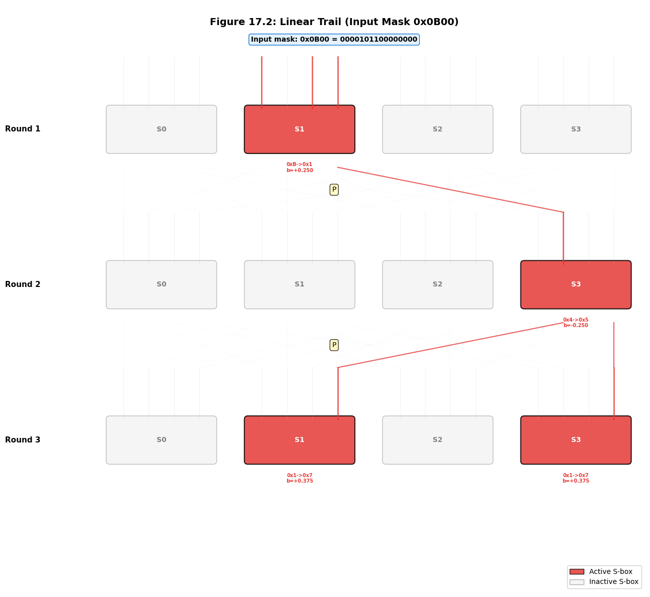
The most famous trail from Heys’ tutorial uses input mask 0x0B00, which activates only S-box 1 in round 1 with input nibble 0xB = 1011. Let us trace this trail step by step to understand how masks propagate through the SPN.
Note
The Heys tutorial uses a slightly different convention for numbering S-boxes and bits. We follow the convention where S-box 0 is the leftmost (most significant) nibble and bit 0 is the most significant bit. The permutation \(\pi(i) = 4(i \bmod 4) + \lfloor i/4 \rfloor\) transposes the \(4 \times 4\) bit matrix.
import numpy as np
import matplotlib.pyplot as plt

SBOX = np.array([0xE, 0x4, 0xD, 0x1, 0x2, 0xF, 0xB, 0x8,
                 0x3, 0xA, 0x6, 0xC, 0x5, 0x9, 0x0, 0x7], dtype=np.int32)
PERM = np.array([0, 4, 8, 12, 1, 5, 9, 13, 2, 6, 10, 14, 3, 7, 11, 15], dtype=np.int32)

def compute_lat(sbox):
    n = len(sbox)
    lat = np.zeros((n, n), dtype=np.int32)
    for a in range(n):
        for b in range(n):
            count = 0
            for x in range(n):
                if bin(a & x).count('1') % 2 == bin(b & sbox[x]).count('1') % 2:
                    count += 1
            lat[a][b] = count - n // 2
    return lat

LAT = compute_lat(SBOX)

def apply_perm(mask, perm):
    result = 0
    for i in range(16):
        if mask & (1 << (15 - i)):
            result |= (1 << (15 - perm[i]))
    return result

def get_nibble(mask, s):
    return (mask >> (4 * (3 - s))) & 0xF

# === Trace the Heys trail starting from input mask 0x0B00 ===
print("Tracing the Heys Example Linear Trail")
print("=" * 60)

input_mask = 0x0B00
print(f"\nInput mask: 0x{input_mask:04X} = {input_mask:016b}")
print(f"  Active S-boxes: ", end="")
for s in range(4):
    nib = get_nibble(input_mask, s)
    if nib != 0:
        print(f"S-box {s} (nibble 0x{nib:X} = {nib:04b})", end=" ")
print()

# Round 1: S-box 1 has input 0xB
# Find best output for 0xB
in_nib = 0xB
print(f"\n--- Round 1 ---")
print(f"S-box 1 input: 0x{in_nib:X} = {in_nib:04b}")
best_out = max(range(1, 16), key=lambda o: abs(LAT[in_nib][o]))
print(f"Best S-box output: 0x{best_out:X} = {best_out:04b}")
print(f"  LAT[0x{in_nib:X}][0x{best_out:X}] = {LAT[in_nib][best_out]:+d}")
print(f"  Bias = {LAT[in_nib][best_out]/16.0:+.4f}")

round1_output = best_out << 8  # Place in S-box 1 position
print(f"Round 1 S-box output mask: 0x{round1_output:04X} = {round1_output:016b}")

# Apply permutation
round2_input = apply_perm(round1_output, PERM)
print(f"After permutation (Round 2 input): 0x{round2_input:04X} = {round2_input:016b}")
print(f"  Active S-boxes: ", end="")
for s in range(4):
    nib = get_nibble(round2_input, s)
    if nib != 0:
        print(f"S-box {s} (nibble 0x{nib:X} = {nib:04b})", end=" ")
print()

# Round 2
print(f"\n--- Round 2 ---")
round2_out_mask = 0
round2_biases = []
for s in range(4):
    nib = get_nibble(round2_input, s)
    if nib != 0:
        best_out2 = max(range(1, 16), key=lambda o: abs(LAT[nib][o]))
        bias2 = LAT[nib][best_out2] / 16.0
        round2_biases.append(bias2)
        round2_out_mask |= (best_out2 << (4 * (3 - s)))
        print(f"  S-box {s}: in=0x{nib:X} -> out=0x{best_out2:X}, bias={bias2:+.4f}")

print(f"Round 2 S-box output mask: 0x{round2_out_mask:04X} = {round2_out_mask:016b}")

# Apply permutation
round3_input = apply_perm(round2_out_mask, PERM)
print(f"After permutation (Round 3 input): 0x{round3_input:04X} = {round3_input:016b}")

# Round 3
print(f"\n--- Round 3 ---")
round3_out_mask = 0
round3_biases = []
for s in range(4):
    nib = get_nibble(round3_input, s)
    if nib != 0:
        best_out3 = max(range(1, 16), key=lambda o: abs(LAT[nib][o]))
        bias3 = LAT[nib][best_out3] / 16.0
        round3_biases.append(bias3)
        round3_out_mask |= (best_out3 << (4 * (3 - s)))
        print(f"  S-box {s}: in=0x{nib:X} -> out=0x{best_out3:X}, bias={bias3:+.4f}")

print(f"Round 3 S-box output mask: 0x{round3_out_mask:04X} = {round3_out_mask:016b}")

# Compute trail bias
all_biases = [LAT[0xB][max(range(1,16), key=lambda o: abs(LAT[0xB][o]))] / 16.0]
all_biases.extend(round2_biases)
all_biases.extend(round3_biases)
total_active = len(all_biases)
trail_bias = 2 ** (total_active - 1)
for b in all_biases:
    trail_bias *= b

print(f"\n=== Trail Summary ===")
print(f"Total active S-boxes: {total_active}")
print(f"Individual biases: {[f'{b:+.4f}' for b in all_biases]}")
print(f"Trail bias = 2^{total_active - 1} * " + " * ".join(f"({b:+.4f})" for b in all_biases))
print(f"           = {trail_bias:+.6f}")
Tracing the Heys Example Linear Trail
============================================================

Input mask: 0x0B00 = 0000101100000000
  Active S-boxes: S-box 1 (nibble 0xB = 1011)

--- Round 1 ---
S-box 1 input: 0xB = 1011
Best S-box output: 0x1 = 0001
  LAT[0xB][0x1] = +4
  Bias = +0.2500
Round 1 S-box output mask: 0x0100 = 0000000100000000
After permutation (Round 2 input): 0x0004 = 0000000000000100
  Active S-boxes: S-box 3 (nibble 0x4 = 0100)

--- Round 2 ---
  S-box 3: in=0x4 -> out=0x5, bias=-0.2500
Round 2 S-box output mask: 0x0005 = 0000000000000101
After permutation (Round 3 input): 0x0101 = 0000000100000001

--- Round 3 ---
  S-box 1: in=0x1 -> out=0x7, bias=+0.3750
  S-box 3: in=0x1 -> out=0x7, bias=+0.3750
Round 3 S-box output mask: 0x0707 = 0000011100000111

=== Trail Summary ===
Total active S-boxes: 4
Individual biases: ['+0.2500', '-0.2500', '+0.3750', '+0.3750']
Trail bias = 2^3 * (+0.2500) * (-0.2500) * (+0.3750) * (+0.3750)
           = -0.070312
17.7 Visualizing Linear Trails Through the SPN#
A visual representation of a linear trail makes the mask propagation through the SPN structure immediately clear. Active S-boxes are highlighted, and the connecting wires show how the permutation spreads bits across S-boxes in subsequent rounds.
Show code cell source
import numpy as np
import matplotlib.pyplot as plt
import matplotlib.patches as mpatches

SBOX = np.array([0xE, 0x4, 0xD, 0x1, 0x2, 0xF, 0xB, 0x8,
                 0x3, 0xA, 0x6, 0xC, 0x5, 0x9, 0x0, 0x7], dtype=np.int32)
PERM = np.array([0, 4, 8, 12, 1, 5, 9, 13, 2, 6, 10, 14, 3, 7, 11, 15], dtype=np.int32)

def compute_lat(sbox):
    n = len(sbox)
    lat = np.zeros((n, n), dtype=np.int32)
    for a in range(n):
        for b in range(n):
            count = 0
            for x in range(n):
                if bin(a & x).count('1') % 2 == bin(b & sbox[x]).count('1') % 2:
                    count += 1
            lat[a][b] = count - n // 2
    return lat

LAT = compute_lat(SBOX)

def get_nibble(mask, s):
    return (mask >> (4 * (3 - s))) & 0xF

def apply_perm(mask, perm):
    result = 0
    for i in range(16):
        if mask & (1 << (15 - i)):
            result |= (1 << (15 - perm[i]))
    return result

# Define trail masks (using the Heys example)
# We construct a 3-round trail with input 0x0B00
input_mask = 0x0B00
# Round 1: S-box 1 in=0xB, best out from LAT
r1_out_nib = max(range(1, 16), key=lambda o: abs(LAT[0xB][o]))
r1_output = r1_out_nib << 8
r2_input = apply_perm(r1_output, PERM)

# Round 2: find best outputs
r2_output = 0
for s in range(4):
    nib = get_nibble(r2_input, s)
    if nib != 0:
        best = max(range(1, 16), key=lambda o: abs(LAT[nib][o]))
        r2_output |= (best << (4 * (3 - s)))

r3_input = apply_perm(r2_output, PERM)

# Round 3: find best outputs
r3_output = 0
for s in range(4):
    nib = get_nibble(r3_input, s)
    if nib != 0:
        best = max(range(1, 16), key=lambda o: abs(LAT[nib][o]))
        r3_output |= (best << (4 * (3 - s)))

round_data = [
    (input_mask, r1_output),
    (r2_input, r2_output),
    (r3_input, r3_output),
]

fig, ax = plt.subplots(figsize=(14, 12))
ax.set_xlim(-1, 17)
ax.set_ylim(-1, 16)
ax.set_aspect('equal')
ax.axis('off')
fig.patch.set_facecolor('white')

# Colors
active_color = '#E53935'
inactive_color = '#E0E0E0'
wire_active = '#E53935'
wire_inactive = '#BDBDBD'
key_color = '#64B5F6'

# Layout parameters
sbox_width = 3.0
sbox_height = 1.2
sbox_gap = 1.0
round_height = 4.5
y_start = 14.5

# Draw title
ax.text(8, 15.5, f'Figure 17.2: Linear Trail (Input Mask 0x{input_mask:04X})',
        fontsize=14, fontweight='bold', ha='center', va='center')

for r_idx, (r_in, r_out) in enumerate(round_data):
    y_top = y_start - r_idx * round_height
    y_sbox = y_top - 1.5
    y_bottom = y_sbox - sbox_height

    # Round label
    ax.text(-0.5, y_sbox - sbox_height / 2, f'Round {r_idx + 1}',
            fontsize=11, fontweight='bold', ha='right', va='center', rotation=0)

    # Draw 4 S-boxes
    for s in range(4):
        in_nib = get_nibble(r_in, s)
        out_nib = get_nibble(r_out, s)
        is_active = in_nib != 0

        x_left = 1.5 + s * (sbox_width + sbox_gap)
        color = active_color if is_active else inactive_color
        alpha = 0.85 if is_active else 0.3

        rect = mpatches.FancyBboxPatch(
            (x_left, y_sbox - sbox_height), sbox_width, sbox_height,
            boxstyle="round,pad=0.1", facecolor=color, edgecolor='black',
            linewidth=1.5 if is_active else 0.8, alpha=alpha
        )
        ax.add_patch(rect)

        label = f'S{s}'
        text_color = 'white' if is_active else 'gray'
        ax.text(x_left + sbox_width / 2, y_sbox - sbox_height / 2,
                label, fontsize=10, fontweight='bold', ha='center', va='center',
                color=text_color)

        if is_active:
            bias = LAT[in_nib][out_nib] / 16.0
            ax.text(x_left + sbox_width / 2, y_sbox - sbox_height - 0.35,
                    f'0x{in_nib:X}->0x{out_nib:X}\nb={bias:+.3f}',
                    fontsize=7, ha='center', va='top', color=active_color,
                    fontweight='bold')

        # Draw input wires (4 per S-box)
        for bit in range(4):
            bit_idx = s * 4 + bit
            x_wire = x_left + 0.4 + bit * (sbox_width - 0.8) / 3
            is_bit_active = (r_in >> (15 - bit_idx)) & 1
            wire_color = wire_active if is_bit_active else wire_inactive
            wire_lw = 2.0 if is_bit_active else 0.5
            ax.plot([x_wire, x_wire], [y_top, y_sbox],
                    color=wire_color, lw=wire_lw, alpha=0.8 if is_bit_active else 0.3)

    # Draw permutation wires between rounds
    if r_idx < len(round_data) - 1:
        y_perm_top = y_bottom - 0.5
        y_perm_bottom = y_start - (r_idx + 1) * round_height

        for bit in range(16):
            src_sbox = bit // 4
            src_bit = bit % 4
            dst_bit = PERM[bit]
            dst_sbox = dst_bit // 4
            dst_bit_in_sbox = dst_bit % 4

            x_src = 1.5 + src_sbox * (sbox_width + sbox_gap) + 0.4 + src_bit * (sbox_width - 0.8) / 3
            x_dst = 1.5 + dst_sbox * (sbox_width + sbox_gap) + 0.4 + dst_bit_in_sbox * (sbox_width - 0.8) / 3

            is_bit_active = (r_out >> (15 - bit)) & 1
            wire_color = wire_active if is_bit_active else wire_inactive
            wire_lw = 1.5 if is_bit_active else 0.3
            wire_alpha = 0.8 if is_bit_active else 0.15

            ax.plot([x_src, x_dst], [y_perm_top, y_perm_bottom],
                    color=wire_color, lw=wire_lw, alpha=wire_alpha)

        # Permutation label
        ax.text(8, (y_perm_top + y_perm_bottom) / 2,
                'P', fontsize=10, ha='center', va='center',
                bbox=dict(boxstyle='round,pad=0.3', facecolor='#FFF9C4',
                         edgecolor='black', linewidth=0.8))

# Input mask label at top
ax.text(8, y_start + 0.5, f'Input mask: 0x{input_mask:04X} = {input_mask:016b}',
        fontsize=10, ha='center', va='center', fontweight='bold',
        bbox=dict(boxstyle='round,pad=0.3', facecolor='#E3F2FD', edgecolor='#1976D2'))

# Legend
legend_elements = [
    mpatches.Patch(facecolor=active_color, edgecolor='black', alpha=0.85, label='Active S-box'),
    mpatches.Patch(facecolor=inactive_color, edgecolor='black', alpha=0.3, label='Inactive S-box'),
]
ax.legend(handles=legend_elements, loc='lower right', fontsize=10, framealpha=0.9)

plt.tight_layout()
plt.savefig('fig_17_2_trail_visualization.png', dpi=150, bbox_inches='tight', facecolor='white')
plt.show()
17.8 Active S-box Count Distribution#
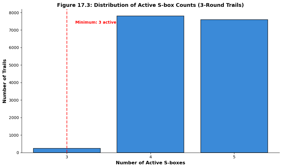
A critical metric for evaluating an SPN’s resistance to linear cryptanalysis is the minimum number of active S-boxes across all possible linear trails. This quantity determines the maximum trail bias and hence the data complexity of the best linear attack.
The following experiment counts active S-boxes for all valid single-active-per-round trails through 3 rounds, producing a histogram that reveals the distribution.
Show code cell source
import numpy as np
import matplotlib.pyplot as plt

SBOX = np.array([0xE, 0x4, 0xD, 0x1, 0x2, 0xF, 0xB, 0x8,
                 0x3, 0xA, 0x6, 0xC, 0x5, 0x9, 0x0, 0x7], dtype=np.int32)
PERM = np.array([0, 4, 8, 12, 1, 5, 9, 13, 2, 6, 10, 14, 3, 7, 11, 15], dtype=np.int32)

def compute_lat(sbox):
    n = len(sbox)
    lat = np.zeros((n, n), dtype=np.int32)
    for a in range(n):
        for b in range(n):
            count = 0
            for x in range(n):
                if bin(a & x).count('1') % 2 == bin(b & sbox[x]).count('1') % 2:
                    count += 1
            lat[a][b] = count - n // 2
    return lat

LAT = compute_lat(SBOX)

def get_nibble(mask, s):
    return (mask >> (4 * (3 - s))) & 0xF

def apply_perm(mask):
    result = 0
    for i in range(16):
        if mask & (1 << (15 - i)):
            result |= (1 << (15 - PERM[i]))
    return result

def count_active_sboxes(mask):
    return sum(1 for s in range(4) if get_nibble(mask, s) != 0)

# Exhaustive enumeration of 3-round trails
# For each input mask, for each valid S-box output combination, trace through 3 rounds
active_counts = []
trail_biases = []
num_valid = 0

# Iterate over all non-zero input masks (only consider those with <= 2 active S-boxes)
for input_mask in range(1, 0x10000):
    r1_active = count_active_sboxes(input_mask)
    if r1_active > 2:
        continue

    # Round 1: enumerate outputs
    r1_nibs = [get_nibble(input_mask, s) for s in range(4)]
    r1_options = []
    for s in range(4):
        if r1_nibs[s] == 0:
            r1_options.append([(0, 0.0)])
        else:
            opts = []
            for out in range(1, 16):
                if abs(LAT[r1_nibs[s]][out]) >= 2:
                    opts.append((out, LAT[r1_nibs[s]][out] / 16.0))
            if not opts:
                r1_options.append([])
            else:
                r1_options.append(opts)

    if any(len(o) == 0 for o in r1_options):
        continue

    for o0, b0 in r1_options[0]:
        for o1, b1 in r1_options[1]:
            for o2, b2 in r1_options[2]:
                for o3, b3 in r1_options[3]:
                    r1_out = (o0 << 12) | (o1 << 8) | (o2 << 4) | o3
                    if r1_out == 0:
                        continue
                    r2_in = apply_perm(r1_out)
                    r2_active = count_active_sboxes(r2_in)
                    if r2_active > 2:
                        continue

                    # Round 2
                    r2_nibs = [get_nibble(r2_in, s) for s in range(4)]
                    for s in range(4):
                        if r2_nibs[s] != 0:
                            for out2 in range(1, 16):
                                if abs(LAT[r2_nibs[s]][out2]) >= 2 and r2_active == 1:
                                    r2_out = out2 << (4 * (3 - s))
                                    r3_in = apply_perm(r2_out)
                                    r3_active = count_active_sboxes(r3_in)
                                    if r3_active > 2:
                                        continue

                                    total_active = r1_active + 1 + r3_active
                                    active_counts.append(total_active)
                                    num_valid += 1

print(f"Enumerated {num_valid} valid trail fragments (single-active middle round)")
print(f"Active S-box count distribution:")

if active_counts:
    counts_arr = np.array(active_counts)
    for val in sorted(set(active_counts)):
        n_trails = np.sum(counts_arr == val)
        print(f"  {val} active S-boxes: {n_trails} trails")

    fig, ax = plt.subplots(figsize=(10, 6))

    bins = np.arange(min(active_counts) - 0.5, max(active_counts) + 1.5, 1)
    ax.hist(active_counts, bins=bins, color='#1976D2', edgecolor='black',
            linewidth=1.2, alpha=0.85, rwidth=0.8)

    ax.set_xlabel('Number of Active S-boxes', fontsize=12, fontweight='bold')
    ax.set_ylabel('Number of Trails', fontsize=12, fontweight='bold')
    ax.set_title('Figure 17.3: Distribution of Active S-box Counts (3-Round Trails)',
                 fontsize=13, fontweight='bold')
    ax.set_xticks(range(min(active_counts), max(active_counts) + 1))
    ax.spines['top'].set_visible(False)
    ax.spines['right'].set_visible(False)

    ax.axvline(x=min(active_counts), color='red', linestyle='--', linewidth=2, alpha=0.7)
    ax.text(min(active_counts) + 0.1, ax.get_ylim()[1] * 0.9,
            f'Minimum: {min(active_counts)} active',
            fontsize=10, color='red', fontweight='bold')

    plt.tight_layout()
    plt.savefig('fig_17_3_active_sbox_distribution.png', dpi=150, bbox_inches='tight', facecolor='white')
    plt.show()
else:
    print("  No valid trails found with current constraints.")
Enumerated 15640 valid trail fragments (single-active middle round)
Active S-box count distribution:
  3 active S-boxes: 240 trails
  4 active S-boxes: 7800 trails
  5 active S-boxes: 7600 trails
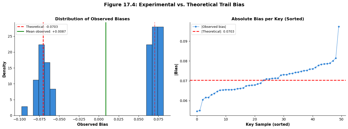
17.9 Experimental Verification of Trail Bias#
The piling-up lemma provides a theoretical prediction for the trail bias under the independent-key assumption. We now verify this prediction experimentally by:
Generating random keys for each round.
Encrypting many random plaintexts through the 3-round SPN.
Checking whether the linear approximation defined by the trail holds.
Comparing the observed bias to the theoretical prediction.
Important
The experimental bias may differ from the theoretical prediction because:
The piling-up lemma assumes independent round keys (which our random keys provide).
The linear hull effect means other trails with the same input/output masks may contribute.
Statistical fluctuations diminish with more samples.
Show code cell source
import numpy as np
import matplotlib.pyplot as plt

SBOX = np.array([0xE, 0x4, 0xD, 0x1, 0x2, 0xF, 0xB, 0x8,
                 0x3, 0xA, 0x6, 0xC, 0x5, 0x9, 0x0, 0x7], dtype=np.int32)
PERM = np.array([0, 4, 8, 12, 1, 5, 9, 13, 2, 6, 10, 14, 3, 7, 11, 15], dtype=np.int32)

def apply_sbox_layer(state, sbox):
    """Apply S-box substitution to each 4-bit nibble."""
    result = 0
    for i in range(4):
        nibble = (state >> (4 * (3 - i))) & 0xF
        result |= sbox[nibble] << (4 * (3 - i))
    return result

def apply_perm_layer(state, perm):
    """Apply bit permutation."""
    result = 0
    for i in range(16):
        if state & (1 << (15 - i)):
            result |= (1 << (15 - perm[i]))
    return result

def encrypt_3rounds(plaintext, round_keys, sbox, perm):
    """Encrypt through 3 rounds of the Heys SPN (no final permutation)."""
    state = plaintext
    for r in range(3):
        state ^= round_keys[r]       # Key mixing
        state = apply_sbox_layer(state, sbox)  # Substitution
        if r < 2:
            state = apply_perm_layer(state, perm)  # Permutation (not in last round)
    state ^= round_keys[3]  # Final key mixing
    return state

def parity(x):
    """Compute parity (XOR of all bits)."""
    p = 0
    while x:
        p ^= x & 1
        x >>= 1
    return p

# Parameters
num_key_samples = 50
num_plaintexts = 10000
input_mask = 0x0B00

# Use a fixed output mask based on the trail we traced
# (we need the output mask after the final round's S-box layer)
# For simplicity, we test the overall input-output approximation
# The output mask corresponds to the last round's output mask from our trail
# We need to try several output masks and find the one that matches

# First, determine the theoretical trail
def compute_lat(sbox):
    n = len(sbox)
    lat = np.zeros((n, n), dtype=np.int32)
    for a in range(n):
        for b in range(n):
            count = 0
            for x in range(n):
                if bin(a & x).count('1') % 2 == bin(b & sbox[x]).count('1') % 2:
                    count += 1
            lat[a][b] = count - n // 2
    return lat

LAT = compute_lat(SBOX)

def get_nibble(mask, s):
    return (mask >> (4 * (3 - s))) & 0xF

def apply_perm(mask):
    result = 0
    for i in range(16):
        if mask & (1 << (15 - i)):
            result |= (1 << (15 - PERM[i]))
    return result

# Trace our best trail to find the output mask
r1_in_nib = get_nibble(input_mask, 1)  # 0xB
r1_out_nib = max(range(1, 16), key=lambda o: abs(LAT[r1_in_nib][o]))
r1_out_mask = r1_out_nib << 8
r2_in_mask = apply_perm(r1_out_mask)

r2_out_mask = 0
r2_biases = []
for s in range(4):
    nib = get_nibble(r2_in_mask, s)
    if nib != 0:
        best = max(range(1, 16), key=lambda o: abs(LAT[nib][o]))
        r2_out_mask |= (best << (4 * (3 - s)))
        r2_biases.append(LAT[nib][best] / 16.0)

r3_in_mask = apply_perm(r2_out_mask)

r3_out_mask = 0
r3_biases = []
for s in range(4):
    nib = get_nibble(r3_in_mask, s)
    if nib != 0:
        best = max(range(1, 16), key=lambda o: abs(LAT[nib][o]))
        r3_out_mask |= (best << (4 * (3 - s)))
        r3_biases.append(LAT[nib][best] / 16.0)

output_mask = r3_out_mask

# Compute theoretical bias
all_biases = [LAT[r1_in_nib][r1_out_nib] / 16.0] + r2_biases + r3_biases
total_active = len(all_biases)
theoretical_bias = 2 ** (total_active - 1)
for b in all_biases:
    theoretical_bias *= b

print(f"Trail: input mask 0x{input_mask:04X}, output mask 0x{output_mask:04X}")
print(f"Active S-boxes: {total_active}")
print(f"Theoretical trail bias: {theoretical_bias:+.6f}")
print(f"\nNote: The experimental bias includes contributions from ALL trails")
print(f"(the linear hull), not just this single trail.\n")

# Run experiment
rng = np.random.default_rng(42)
observed_biases = []

for key_trial in range(num_key_samples):
    round_keys = rng.integers(0, 0x10000, size=4)

    count_match = 0
    for _ in range(num_plaintexts):
        pt = rng.integers(0, 0x10000)
        ct = encrypt_3rounds(int(pt), round_keys, SBOX, PERM)

        pt_parity = parity(int(pt) & input_mask)
        ct_parity = parity(ct & output_mask)

        if pt_parity == ct_parity:
            count_match += 1

    obs_bias = count_match / num_plaintexts - 0.5
    observed_biases.append(obs_bias)

obs_arr = np.array(observed_biases)
print(f"Experimental results ({num_key_samples} random key samples, {num_plaintexts} plaintexts each):")
print(f"  Mean observed bias:   {np.mean(obs_arr):+.6f}")
print(f"  Std of observed bias: {float(np.std(obs_arr)):.6f}")
print(f"  Mean |observed bias|: {float(np.mean(np.abs(obs_arr))):.6f}")
print(f"  Theoretical |bias|:   {float(abs(theoretical_bias)):.6f}")

fig, axes = plt.subplots(1, 2, figsize=(14, 5))

# Histogram of observed biases
ax = axes[0]
ax.hist(observed_biases, bins=25, color='#1976D2', edgecolor='black',
        linewidth=0.8, alpha=0.85, density=True)
ax.axvline(x=theoretical_bias, color='red', linestyle='--', linewidth=2,
           label=f'Theoretical: {theoretical_bias:+.4f}')
ax.axvline(x=-theoretical_bias, color='red', linestyle='--', linewidth=2, alpha=0.5)
ax.axvline(x=np.mean(obs_arr), color='green', linestyle='-', linewidth=2,
           label=f'Mean observed: {np.mean(obs_arr):+.4f}')
ax.set_xlabel('Observed Bias', fontsize=11, fontweight='bold')
ax.set_ylabel('Density', fontsize=11, fontweight='bold')
ax.set_title('Distribution of Observed Biases', fontsize=12, fontweight='bold')
ax.legend(fontsize=9)
ax.spines['top'].set_visible(False)
ax.spines['right'].set_visible(False)

# Absolute bias comparison
ax = axes[1]
sorted_abs = np.sort(np.abs(observed_biases))
ax.plot(range(len(sorted_abs)), sorted_abs, 'o-', color='#1976D2',
        markersize=4, linewidth=1, alpha=0.8, label='|Observed bias|')
ax.axhline(y=abs(theoretical_bias), color='red', linestyle='--', linewidth=2,
           label=f'|Theoretical|: {float(abs(theoretical_bias)):.4f}')
ax.set_xlabel('Key Sample (sorted)', fontsize=11, fontweight='bold')
ax.set_ylabel('|Bias|', fontsize=11, fontweight='bold')
ax.set_title('Absolute Bias per Key (Sorted)', fontsize=12, fontweight='bold')
ax.legend(fontsize=9)
ax.spines['top'].set_visible(False)
ax.spines['right'].set_visible(False)

fig.suptitle('Figure 17.4: Experimental vs. Theoretical Trail Bias',
             fontsize=14, fontweight='bold', y=1.02)

plt.tight_layout()
plt.savefig('fig_17_4_experimental_bias.png', dpi=150, bbox_inches='tight', facecolor='white')
plt.show()
Trail: input mask 0x0B00, output mask 0x0707
Active S-boxes: 4
Theoretical trail bias: -0.070312

Note: The experimental bias includes contributions from ALL trails
(the linear hull), not just this single trail.
Experimental results (50 random key samples, 10000 plaintexts each):
  Mean observed bias:   +0.008696
  Std of observed bias: 0.070429
  Mean |observed bias|: 0.070596
  Theoretical |bias|:   0.070312
17.10 The Bias Magnitude Landscape#
To understand how the choice of input mask affects the maximum achievable trail bias, we scan all possible single-nibble input masks and compute the best trail bias achievable in 2 rounds. This produces a landscape showing which input masks are most promising for linear cryptanalysis.
Show code cell source
import numpy as np
import matplotlib.pyplot as plt

SBOX = np.array([0xE, 0x4, 0xD, 0x1, 0x2, 0xF, 0xB, 0x8,
                 0x3, 0xA, 0x6, 0xC, 0x5, 0x9, 0x0, 0x7], dtype=np.int32)
PERM = np.array([0, 4, 8, 12, 1, 5, 9, 13, 2, 6, 10, 14, 3, 7, 11, 15], dtype=np.int32)

def compute_lat(sbox):
    n = len(sbox)
    lat = np.zeros((n, n), dtype=np.int32)
    for a in range(n):
        for b in range(n):
            count = 0
            for x in range(n):
                if bin(a & x).count('1') % 2 == bin(b & sbox[x]).count('1') % 2:
                    count += 1
            lat[a][b] = count - n // 2
    return lat

LAT = compute_lat(SBOX)

def get_nibble(mask, s):
    return (mask >> (4 * (3 - s))) & 0xF

def apply_perm(mask):
    result = 0
    for i in range(16):
        if mask & (1 << (15 - i)):
            result |= (1 << (15 - PERM[i]))
    return result

# For each of the 4 S-box positions and each non-zero nibble value,
# compute the best 2-round trail bias
results = np.zeros((4, 15))  # 4 positions x 15 non-zero nibbles

for pos in range(4):
    for nib_idx, in_nib in enumerate(range(1, 16)):
        input_mask = in_nib << (4 * (3 - pos))

        best_bias = 0
        # Round 1: try all outputs
        for out1 in range(1, 16):
            if LAT[in_nib][out1] == 0:
                continue
            b1 = LAT[in_nib][out1] / 16.0

            r1_out = out1 << (4 * (3 - pos))
            r2_in = apply_perm(r1_out)

            # Round 2: find best single S-box output
            for s2 in range(4):
                nib2 = get_nibble(r2_in, s2)
                if nib2 == 0:
                    continue

                # Check if only one S-box is active in round 2
                if sum(1 for ss in range(4) if get_nibble(r2_in, ss) != 0) == 1:
                    for out2 in range(1, 16):
                        if LAT[nib2][out2] == 0:
                            continue
                        b2 = LAT[nib2][out2] / 16.0

                        trail_bias = 2 * b1 * b2  # 2^(2-1) * b1 * b2
                        if abs(trail_bias) > abs(best_bias):
                            best_bias = trail_bias

        results[pos, nib_idx] = abs(best_bias)

fig, ax = plt.subplots(figsize=(12, 6))

im = ax.imshow(results, cmap='YlOrRd', aspect='auto', vmin=0)
ax.set_xticks(range(15))
ax.set_xticklabels([f'0x{i:X}' for i in range(1, 16)], fontsize=8)
ax.set_yticks(range(4))
ax.set_yticklabels([f'S-box {i}' for i in range(4)], fontsize=10)
ax.set_xlabel('Input Nibble Value', fontsize=12, fontweight='bold')
ax.set_ylabel('S-box Position', fontsize=12, fontweight='bold')
ax.set_title('Figure 17.5: Best 2-Round Trail |Bias| by Input Nibble',
             fontsize=13, fontweight='bold')

for i in range(4):
    for j in range(15):
        val = results[i, j]
        color = 'white' if val > 0.02 else 'black'
        ax.text(j, i, f'{float(val):.3f}', ha='center', va='center', fontsize=7,
                color=color, fontweight='bold')

cbar = fig.colorbar(im, ax=ax, shrink=0.8)
cbar.set_label('|Trail Bias|', fontsize=11)

plt.tight_layout()
plt.savefig('fig_17_5_bias_landscape.png', dpi=150, bbox_inches='tight', facecolor='white')
plt.show()

# Find the overall best
best_pos = np.unravel_index(np.argmax(results), results.shape)
best_nib = best_pos[1] + 1
print(f"\nBest 2-round trail: S-box {best_pos[0]}, input nibble 0x{best_nib:X}")
print(f"  |Bias| = {float(results[best_pos]):.6f}")
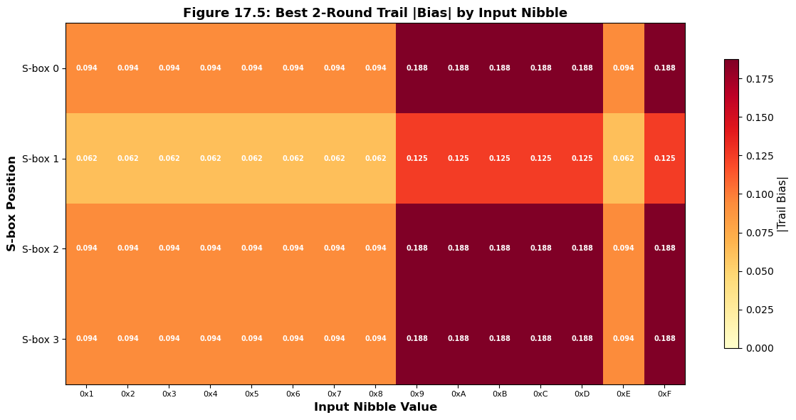
Best 2-round trail: S-box 0, input nibble 0x9
  |Bias| = 0.187500
17.11 Effect of Active S-box Count on Trail Bias#
The piling-up lemma shows that trail bias decreases exponentially with the number of active S-boxes. Specifically, if each active S-box contributes a bias of magnitude \(\varepsilon\), the trail bias scales as:
For the Heys S-box, the maximum single-S-box bias is \(|\varepsilon_{\max}| = 6/16 = 0.375\). The following plot shows how the maximum possible trail bias decays as the number of active S-boxes increases.
Show code cell source
import numpy as np
import matplotlib.pyplot as plt

# Maximum single S-box bias for the Heys S-box
eps_max = 6 / 16  # = 0.375

# Trail bias as function of number of active S-boxes
active_range = np.arange(1, 13)
max_trail_bias = np.array([2**(a - 1) * eps_max**a for a in active_range])

# For comparison: if all biases were the minimum non-zero value
eps_min = 2 / 16  # = 0.125
min_trail_bias = np.array([2**(a - 1) * eps_min**a for a in active_range])

# Data complexity ~ 1/bias^2
data_complexity_max = 1.0 / max_trail_bias**2
data_complexity_min = 1.0 / min_trail_bias**2

fig, axes = plt.subplots(1, 2, figsize=(14, 5.5))

# Left: Trail bias vs active S-boxes
ax = axes[0]
ax.semilogy(active_range, max_trail_bias, 'o-', color='#D32F2F', linewidth=2,
            markersize=8, label=f'Max bias ($\\varepsilon$ = {float(eps_max):.3f})')
ax.semilogy(active_range, min_trail_bias, 's--', color='#1976D2', linewidth=2,
            markersize=8, label=f'Min bias ($\\varepsilon$ = {float(eps_min):.3f})')
ax.set_xlabel('Number of Active S-boxes ($a$)', fontsize=12, fontweight='bold')
ax.set_ylabel('|Trail Bias|', fontsize=12, fontweight='bold')
ax.set_title('Trail Bias vs. Active S-boxes', fontsize=12, fontweight='bold')
ax.legend(fontsize=10)
ax.grid(True, alpha=0.3)
ax.set_xticks(active_range)
ax.spines['top'].set_visible(False)
ax.spines['right'].set_visible(False)

# Right: Data complexity vs active S-boxes
ax = axes[1]
ax.semilogy(active_range, data_complexity_max, 'o-', color='#D32F2F', linewidth=2,
            markersize=8, label=f'Best case ($\\varepsilon$ = {float(eps_max):.3f})')
ax.semilogy(active_range, data_complexity_min, 's--', color='#1976D2', linewidth=2,
            markersize=8, label=f'Worst case ($\\varepsilon$ = {float(eps_min):.3f})')

# Mark typical block sizes
ax.axhline(y=2**16, color='gray', linestyle=':', alpha=0.5)
ax.text(11, 2**16 * 1.5, '$2^{16}$ (full codebook)', fontsize=8, color='gray')
ax.axhline(y=2**43, color='green', linestyle=':', alpha=0.5)
ax.text(11, 2**43 * 1.5, '$2^{43}$ (Matsui\'s DES attack)', fontsize=8, color='green')

ax.set_xlabel('Number of Active S-boxes ($a$)', fontsize=12, fontweight='bold')
ax.set_ylabel('Data Complexity ($\\approx 1/\\varepsilon^2$)', fontsize=12, fontweight='bold')
ax.set_title('Data Complexity vs. Active S-boxes', fontsize=12, fontweight='bold')
ax.legend(fontsize=10)
ax.grid(True, alpha=0.3)
ax.set_xticks(active_range)
ax.spines['top'].set_visible(False)
ax.spines['right'].set_visible(False)

fig.suptitle('Figure 17.6: Impact of Active S-box Count on Attack Feasibility',
             fontsize=14, fontweight='bold', y=1.02)

plt.tight_layout()
plt.savefig('fig_17_6_active_sbox_impact.png', dpi=150, bbox_inches='tight', facecolor='white')
plt.show()

print("Data complexity estimates (known plaintexts needed):")
print(f"{'Active S-boxes':>16s} {'Best case':>14s} {'Worst case':>14s}")
print("-" * 48)
for a, dc_max, dc_min in zip(active_range, data_complexity_max, data_complexity_min):
    print(f"{int(a):>16d}   2^{float(np.log2(dc_max)):>5.1f}       2^{float(np.log2(dc_min)):>5.1f}")
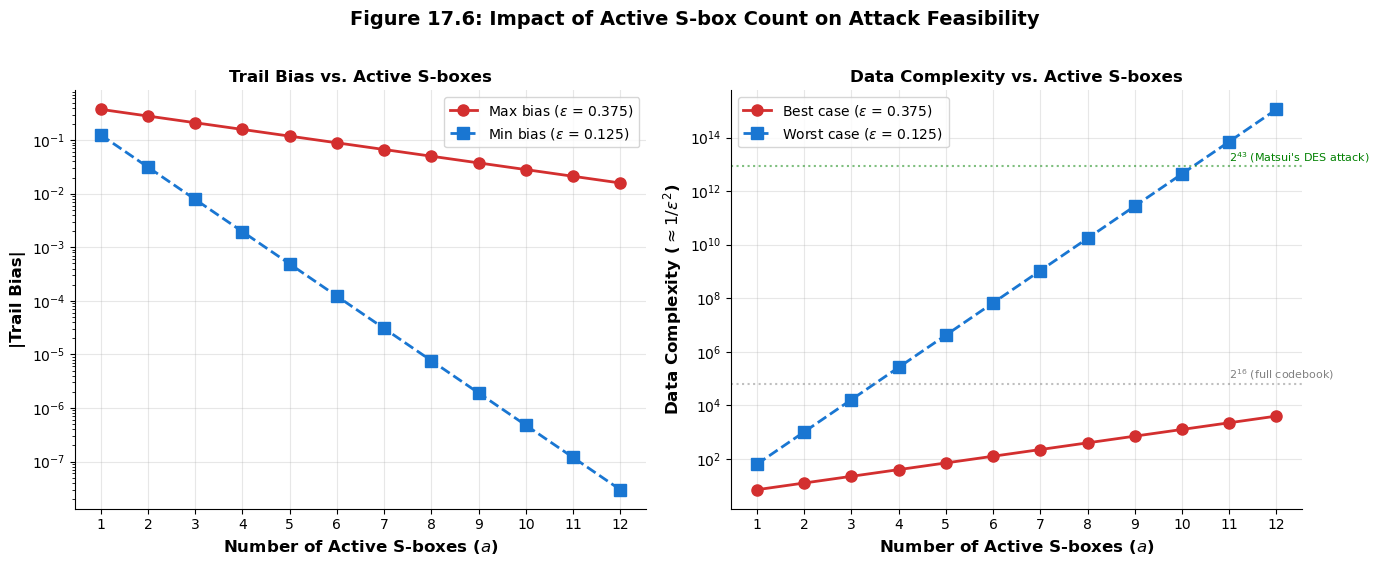
Data complexity estimates (known plaintexts needed):
  Active S-boxes      Best case     Worst case
------------------------------------------------
               1   2^  2.8       2^  6.0
               2   2^  3.7       2^ 10.0
               3   2^  4.5       2^ 14.0
               4   2^  5.3       2^ 18.0
               5   2^  6.2       2^ 22.0
               6   2^  7.0       2^ 26.0
               7   2^  7.8       2^ 30.0
               8   2^  8.6       2^ 34.0
               9   2^  9.5       2^ 38.0
              10   2^ 10.3       2^ 42.0
              11   2^ 11.1       2^ 46.0
              12   2^ 12.0       2^ 50.0
17.12 Exercises#
The following exercises reinforce the concepts of linear trail construction, bias computation, and systematic search.
Exercise 17.1 (Manual Trail Tracing).
Consider the input mask \(\alpha_0 = \texttt{0x0500}\) (binary: 0000 0101 0000 0000).
(a) Identify which S-boxes are active in round 1. (b) Using the LAT, find the output mask for round 1 that maximizes \(|\text{bias}|\). (c) Apply the bit permutation and determine the round 2 input mask. (d) Trace the trail through round 2, again choosing the maximum-bias output. (e) Compute the overall 2-round trail bias using the piling-up lemma.
Hint
The input mask 0x0500 has S-box 1 active with nibble 0x5 = 0101. Look up row 0x5 in the LAT to find which output nibble has the largest absolute entry. After applying the permutation \(\pi(i) = 4(i \bmod 4) + \lfloor i/4 \rfloor\), determine which S-boxes become active in round 2. Remember: the permutation acts on bit positions, not on nibble values.
Exercise 17.2 (Counting Valid Trails). For the Heys SPN with the given S-box and permutation:
(a) How many valid 1-round trails exist with exactly 1 active S-box? (Count distinct (input mask, output mask) pairs with non-zero LAT entry.) (b) How many valid 1-round trails exist with exactly 2 active S-boxes? (c) Explain why the permutation layer does not affect the number of valid 1-round trails but critically affects multi-round trail counts.
Hint
For part (a): there are 4 S-box positions, and each can have any of the 15 non-zero input nibbles. For each input nibble, count how many non-zero entries exist in the corresponding LAT row (excluding column 0). For part (c): the permutation redistributes bits between S-boxes, so a single active S-box in one round may activate multiple S-boxes in the next round.
Exercise 17.3 (Piling-Up Verification).
For the 3-round trail starting with input mask 0x0004:
(a) Trace the trail through all 3 rounds, choosing maximum-bias outputs at each S-box. (b) Compute the theoretical trail bias. (c) Write a Python program to verify this bias experimentally using 50,000 random plaintexts and 20 random keys. (d) Plot the distribution of observed biases across the 20 key samples.
Hint
Input mask 0x0004 activates S-box 3 with nibble 0x4 = 0100 in the rightmost position. The best output for this nibble can be found from LAT[4][:]. Use the encrypt_3rounds function from the experimental verification section, but modify the input and output masks. The experimental bias should cluster around the theoretical value (possibly with opposite sign for some keys, due to key-dependent sign flipping).
Exercise 17.4 (Linear Hull Effect).
Consider the input mask 0x0B00 and the output mask you found for the 3-round trail in Section 17.6.
(a) Find at least two additional distinct trails (different intermediate masks) that connect the same input and output masks. (b) Compute the bias of each additional trail. (c) Under the linear hull model, the total bias is \(\varepsilon_{\text{hull}} = \sum_{\mathcal{T}} \varepsilon_{\mathcal{T}}\) where the sum ranges over all trails \(\mathcal{T}\). Compute the hull bias using your trails from parts (a) and (b). (d) Compare the hull bias to the single-trail bias. Is the hull effect constructive or destructive?
Hint
To find alternative trails, change the output mask at one or more intermediate S-boxes. For instance, in round 1, instead of choosing the maximum-bias output for S-box 1, try the second-best or third-best output. Then re-trace through rounds 2 and 3. Not all alternative paths will be valid (some may have zero-bias entries), so you need to check. The hull effect depends on whether the individual trail biases have the same or opposite signs.
Exercise 17.5 (Challenge: Minimum Active S-boxes and the Wide Trail Strategy). The wide trail strategy (Daemen and Rijmen, 1999) is a design principle that maximizes the minimum number of active S-boxes across all possible linear (and differential) trails.
(a) For the Heys SPN permutation \(\pi(i) = 4(i \bmod 4) + \lfloor i/4 \rfloor\), find the minimum number of active S-boxes over all valid 2-round linear trails. (You may use a computer search.) (b) Now consider the identity permutation \(\pi(i) = i\) (no bit mixing between S-boxes). Find the minimum number of active S-boxes for 2-round trails. (c) Explain the dramatic difference between (a) and (b) in terms of diffusion. (d) The AES uses a linear mixing layer (MixColumns) that guarantees at least 5 active S-boxes in any 4-round trail. If each AES S-box has maximum bias \(2^{-3}\), what is the maximum 4-round trail bias? How many known plaintexts would this require?
Hint
For (b) with the identity permutation, each S-box in round 2 receives exactly the output of the corresponding S-box in round 1. This means a trail can have just 1 active S-box in each round (total: 2), giving a very high trail bias. For (a), the Heys permutation disperses each S-box’s output bits across all four S-boxes, forcing more active S-boxes in round 2. For (d), use the formula \(\varepsilon_{\text{trail}} = 2^{a-1} \cdot \prod \varepsilon_i\) with \(a = 5\) and \(\varepsilon_i = 2^{-3}\).
17.13 Summary and Key Takeaways#
This chapter has developed the theory and practice of linear trail construction – the systematic process of finding exploitable linear approximations through multi-round SPNs.
Key takeaways:
A linear trail is a sequence of masks \(\mathcal{T} = (\alpha_0, \alpha_1, \ldots, \alpha_r)\) that specifies the exact propagation path of a linear approximation through \(r\) rounds. At each round, the trail passes through active S-boxes (where the input mask is non-zero) and collects a bias from the LAT.
The piling-up lemma governs trail bias composition: \(\varepsilon_{\text{trail}} = 2^{a-1} \prod_{i=1}^a \varepsilon_i\), where \(a\) is the number of active S-boxes. This exponential scaling means that minimizing active S-boxes is the primary design goal for resistance to linear cryptanalysis.
The bit permutation is critical for security. A well-designed permutation (like the Heys permutation or AES’s ShiftRows + MixColumns) ensures that even a single active S-box in one round forces multiple active S-boxes in subsequent rounds. The wide trail strategy formalizes this principle.
Linear hulls (Nyberg, 1994) aggregate the contributions of all trails connecting the same input and output masks. The single-trail bias can either overestimate or underestimate the true linear hull bias, depending on whether trails interfere constructively or destructively.
Experimental verification confirms the theoretical predictions under the independent-key assumption, while also revealing the variance introduced by key-dependent effects.
Tip
Looking ahead. In Chapter 18, we will use the linear trails constructed here to mount a complete Matsui’s Algorithm 2 attack on the Heys SPN, recovering the last round key from known plaintext-ciphertext pairs. The quality of the trails found in this chapter directly determines the number of known plaintexts required for the attack to succeed.
17.14 References#
Mitsuru Matsui, “Linear Cryptanalysis Method for DES Cipher,” Advances in Cryptology – EUROCRYPT ‘93, Lecture Notes in Computer Science, vol. 765, pp. 386–397, Springer, 1994. The foundational paper introducing linear cryptanalysis. Matsui demonstrated how to systematically construct linear trails through DES and used them to mount a known-plaintext attack requiring \(2^{43}\) plaintext-ciphertext pairs – the first publicly known attack faster than brute force against DES.
Mitsuru Matsui, “The First Experimental Cryptanalysis of the Data Encryption Standard,” Advances in Cryptology – CRYPTO ‘94, Lecture Notes in Computer Science, vol. 839, pp. 1–11, Springer, 1994. The companion paper reporting the actual implementation and execution of the linear cryptanalysis attack on DES, confirming the theoretical predictions.
Kaisa Nyberg, “Linear Approximation of Block Ciphers,” Advances in Cryptology – EUROCRYPT ‘94, Lecture Notes in Computer Science, vol. 950, pp. 439–444, Springer, 1995. Introduced the concept of linear hulls, showing that the bias of a linear approximation is determined by the sum over all trails, not just the dominant one. This insight had profound implications for both attack and design.
Howard M. Heys, “A Tutorial on Linear and Differential Cryptanalysis,” Cryptologia, 26(3), pp. 189–221, 2002. An excellent pedagogical introduction to linear and differential cryptanalysis using a small SPN as a running example. The S-box, permutation, and trail examples in this chapter follow Heys’ tutorial.
Joan Daemen and Vincent Rijmen, The Design of Rijndael: AES – The Advanced Encryption Standard, Springer, 2002. The definitive reference on AES design, including the wide trail strategy that maximizes the minimum number of active S-boxes to provide provable bounds against linear and differential cryptanalysis.
Eli Biham and Adi Shamir, Differential Cryptanalysis of the Data Encryption Standard, Springer, 1993. While focused on differential cryptanalysis, this book’s systematic approach to trail construction through DES’s Feistel structure inspired Matsui’s parallel development for linear cryptanalysis.