Chapter 30: The Index Calculus Method (SageMath)

Python Version Available

This notebook contains the SageMath implementation. A pure Python/NumPy version is available in Chapter 30: The Index Calculus Method.

30.1 Historical Background: Adleman’s Subexponential Breakthrough

In 1979, Leonard Adleman introduced the index calculus method for solving the discrete logarithm problem (DLP) in the multiplicative group \((\mathbb{Z}/p\mathbb{Z})^*\) of a prime field. The problem is: given a generator \(g\), a prime \(p\), and a target \(h \equiv g^x \pmod{p}\), find the unknown exponent \(x\).

Prior to Adleman’s work, the best generic algorithms for the DLP – such as baby-step/giant-step (Shanks, 1971) and Pollard’s rho (1978) – ran in \(O(\sqrt{p})\) time, which is fully exponential in the bit-length of \(p\). Adleman’s key insight was that the multiplicative group of a prime field has additional structure that generic group algorithms ignore: every element can be lifted to the integers and factored.

The index calculus strategy has three phases:

1. Factor base selection. Choose a set \(\mathcal{B} = \{p_1, p_2, \ldots, p_k\}\) of small primes.

2. Relation collection. Compute powers \(g^r \bmod p\) for random exponents \(r\) and keep those that are \(\mathcal{B}\)-smooth (factorable entirely over \(\mathcal{B}\)). Each such power yields a linear equation in the unknown discrete logarithms \(\log_g p_i \pmod{p-1}\).

3. Individual logarithm. Express \(h \cdot g^s \bmod p\) as a \(\mathcal{B}\)-smooth number for some offset \(s\), then combine with the solved logarithms from phase 2.

This approach achieves subexponential running time, making it dramatically faster than any generic method for large primes. It is the foundational idea behind all modern attacks on the DLP in prime fields, including the number field sieve variants used in practice today.

The state-of-the-art situation in RSA factorization and DLP problems is nicely described in T. Kleinjung et al., “Factorization of a 768-Bit RSA Modulus,” Advances in Cryptology – CRYPTO 2010, LNCS 6223, Springer, 2010. An extensive literature on index calculus methods can be found in the references listed in Section 30.13.

30.2 Core Definitions

30.3 Helper Functions: Factor Base and Smoothness Testing

# Factor base construction using SageMath's Primes()
# SageMath provides direct prime enumeration -- no need for a manual sieve.

pp = Primes()
primes_30 = [pp[i] for i in range(prime_pi(30))]
print(f"Primes up to 30: {primes_30}")
print(f"Count: {len(primes_30)}")

Primes up to 30: [2, 3, 5, 7, 11, 13, 17, 19, 23, 29]
Count: 10

# Build a factor base of small primes using SageMath's iterator
# This uses the Primes iterator for efficient enumeration.

n = 10
pp = Primes()

primes = []
start = 2
while start < n:
    stop = min(start + 10, n)  # Generate primes in batches of size 10
    primes += list(pp.iterator_range(start=start, stop=stop))
    start = stop

print(primes)

# Final set of small primes including 2 and 3
S = [2, 3] + primes
print(f"Factor base S = {S}")

[5, 7, 11, 13, 17, 19, 23, 29]
Factor base S = [2, 3, 5, 7, 11, 13, 17, 19, 23, 29]

# Restricted factorization procedure
# In this function we obtain a partial factorization based on the set S.
# If the factorization is not complete the bool value fin is false.
# This uses SageMath's .valuation() method on ZZ elements.

def FactS(n, S):
    li = dict()
    for p in S:
        k = n.valuation(p)
        li[p] = k
        n //= p**(k)
    if n == 1:
        fin = True
    else:
        fin = False
    return fin, li

# Test: 360 = 2^3 * 3^2 * 5
fb = [2, 3, 5, 7]
smooth, exponents = FactS(ZZ(360), fb)
print(f"Factor base: {fb}")
print(f"360 is smooth: {smooth}, exponents: {exponents}")
print(f"Verification: {prod(p^e for p, e in exponents.items())} == 360")

# Test a non-smooth number: 77 = 7 * 11
smooth2, _ = FactS(ZZ(77), fb)
print(f"77 is smooth over {{2,3,5,7}}: {smooth2}")

Factor base: [2, 3, 5, 7]
360 is smooth: True, exponents: {2: 3, 3: 2, 5: 1, 7: 0}
Verification: 360 == 360
77 is smooth over {2,3,5,7}: False

Implementation Note

In SageMath, the ZZ ring provides the .valuation(p) method that computes the exact \(p\)-adic valuation of an integer – i.e., the largest power of \(p\) dividing it. This makes the restricted factorization over a factor base both concise and efficient. Unlike Python/NumPy, there is no need to implement modular arithmetic or Gaussian elimination from scratch: SageMath’s matrix(ZZ, ...) and module operations handle linear algebra over the integers natively.

30.4 Relation Collection: A Small Example

# We fix a prime (the 101st prime, p = 547)
p = Primes()[100]
print(f"p = {p}")

# We will work strictly in the finite field F_p
F = GF(p)

# Fix a multiplicative generator (this is the setup of the discrete logarithm problem)
g = F.multiplicative_generator()
print(f"Generator g = {g}")

# The goal is to rediscover the value of k from the knowledge of g^k
k = randint(2, p - 1)
h = g**k
print(f"Secret exponent k = {k}")
print(f"Target h = g^k = {h}")

p = 547
Generator g = 2
Secret exponent k = 424
Target h = g^k = 530

# We fix a basis of small primes
# This is a critical step which makes the algorithm very flexible
# (and difficult to implement for large primes)
pp = Primes()
[pp[i] for i in range(10)]

[2, 3, 5, 7, 11, 13, 17, 19, 23, 29]

# This list generates factorization of the lifts of g^k for small k's over the integers
# using only the restricted list of primes S
c = 1
lin = []
for k in range(1, 50):
    c *= g
    complete, li = FactS(ZZ(c), S)  # We use ZZ (ring of integers for the .valuation method)
    if complete:
        lin.append([li[p] for p in S] + [k])

print(f"Found {len(lin)} smooth relations out of 49 trials")
for row in lin[:5]:
    print(row)

Found 22 smooth relations out of 49 trials
[1, 0, 0, 0, 0, 0, 0, 0, 0, 0, 1]
[2, 0, 0, 0, 0, 0, 0, 0, 0, 0, 2]
[3, 0, 0, 0, 0, 0, 0, 0, 0, 0, 3]
[4, 0, 0, 0, 0, 0, 0, 0, 0, 0, 4]
[5, 0, 0, 0, 0, 0, 0, 0, 0, 0, 5]

# We form a matrix of these relations
mm = matrix(lin)
print(f"Relation matrix shape: {mm.nrows()} x {mm.ncols()}")
mm

Relation matrix shape: 22 x 11

22 x 11 dense matrix over Integer Ring (use the '.str()' method to see the entries)

# The row-echelon form has many zero rows, because lots of relations are linearly dependent
# so they are discarded from the final matrix
[r for r in mm.echelon_form().rows() if not (r.is_zero())]

[(1, 0, 0, 0, 0, 0, 0, 0, 0, 0, 1),
 (0, 1, 0, 0, 0, 0, 0, 1, 0, 0, 113),
 (0, 0, 1, 0, 1, 0, 0, 0, 1, 0, -4),
 (0, 0, 0, 1, 1, 0, 0, 1, 1, 0, 150),
 (0, 0, 0, 0, 2, 0, 0, 1, 1, 0, 117),
 (0, 0, 0, 0, 0, 1, 0, 0, 1, 0, 33),
 (0, 0, 0, 0, 0, 0, 1, 1, 1, 0, 128),
 (0, 0, 0, 0, 0, 0, 0, 2, 1, 0, 207),
 (0, 0, 0, 0, 0, 0, 0, 0, 2, 0, 40)]

# This illustrates the sense of the second row above
(pow(2, 113, p)) % p == (3 * 19) % p

True

# We will use the matrix of non-trivial relations further
mm3 = matrix([r for r in mm.echelon_form().rows() if not (r.is_zero())])
print(f"Non-trivial relation matrix: {mm3.nrows()} x {mm3.ncols()}")
mm3

Non-trivial relation matrix: 9 x 11

[  1   0   0   0   0   0   0   0   0   0   1]
[  0   1   0   0   0   0   0   1   0   0 113]
[  0   0   1   0   1   0   0   0   1   0  -4]
[  0   0   0   1   1   0   0   1   1   0 150]
[  0   0   0   0   2   0   0   1   1   0 117]
[  0   0   0   0   0   1   0   0   1   0  33]
[  0   0   0   0   0   0   1   1   1   0 128]
[  0   0   0   0   0   0   0   2   1   0 207]
[  0   0   0   0   0   0   0   0   2   0  40]

# The image of the matrix mm3 is a module spanned by the image vectors
# We produce it with the echelon form matrix, notice that the column
# corresponding to 29 was discarded because it was identically zero
matrix(mm3.columns()[:-2]).image()

Free module of degree 9 and rank 9 over Integer Ring
Echelon basis matrix:
[1 0 0 0 0 0 0 0 0]
[0 1 0 0 0 0 0 0 0]
[0 0 1 0 0 0 0 0 0]
[0 0 0 1 0 0 0 0 0]
[0 0 0 0 1 0 0 0 4]
[0 0 0 0 0 1 0 0 0]
[0 0 0 0 0 0 1 0 0]
[0 0 0 0 0 0 0 1 6]
[0 0 0 0 0 0 0 0 8]

30.5 Experiment 1: Individual Logarithm via Module Membership

Algorithm Correctness

Each smooth relation \(g^r \equiv p_1^{e_1} \cdots p_k^{e_k} \pmod{p}\) translates into the linear congruence

\[ r \equiv e_1 \log_g p_1 + e_2 \log_g p_2 + \cdots + e_k \log_g p_k \pmod{p-1}.\]

With enough such relations (\(\geq k\)), the system is (over)determined and Gaussian elimination mod \(p-1\) recovers the individual logarithms. The correctness of Phase 3 follows from the identity \(\log_g(h \cdot g^s) = \log_g h + s\).

# We want to find out whether we can deduce the exponent 207 from
# the factorization vector of g^207 and our restricted list of primes and relations
v = vector([FactS(ZZ(g^207), S)[1][p] for p in S[:-1]])
print(f"Factorization vector of g^207: {v}")

Factorization vector of g^207: (1, 0, 0, 2, 0, 0, 0, 0, 0)

# Module of relations
M = matrix([vector(x[:-2]) for x in mm3.rows()]).image()
M

Free module of degree 9 and rank 9 over Integer Ring
Echelon basis matrix:
[1 0 0 0 0 0 0 0 0]
[0 1 0 0 0 0 0 1 0]
[0 0 1 0 1 0 0 0 1]
[0 0 0 1 1 0 0 1 1]
[0 0 0 0 2 0 0 1 1]
[0 0 0 0 0 1 0 0 1]
[0 0 0 0 0 0 1 1 1]
[0 0 0 0 0 0 0 2 1]
[0 0 0 0 0 0 0 0 2]

# We check that indeed our vector v can be linearly expressed as the
# combination of the row vectors from the basis of M
M.are_linearly_dependent([vector(x[:-2]) for x in mm3.rows()] + [v])

True

# Using the left kernel of the relation matrix of M we obtain a relation
# which tells us how the vector v is expressed in that basis as the
# combination of the relation vectors
rel = matrix(M.basis() + [v]).left_kernel().basis()[0]

rel[:-1]

(4, 0, 0, 8, -4, 0, 0, -2, -1)

# With the dot product we obtain the exponent a
a = rel[:-1].dot_product(vector(mm3.columns()[-1:][0]))
print(f"Exponent a = {a}")

Exponent a = 282

# This exponent tells us the exponent b such that
# g^a = h^b
# In the case when b = 1, we have already solved the DLP: k = a
# Otherwise we solve a restricted congruence a == k*b (mod p-1)
b = rel[-1]
print(f"Exponent b = {b}")

Exponent b = -4

# Verify: g^282 should equal (g^207)^4 if b = 4 (or similar relation)
print(f"g^(282) = {g^(282)}")
print(f"(g^(207))^4 = {(g^(207))^4}")

g^(282) = 35
(g^(207))^4 = 35

30.6 Experiment 2: Full Index Calculus on a ~31-bit Prime

We now summarize the full procedure and apply it to a substantially larger prime. This demonstrates the scalability of the method with SageMath’s native integer arithmetic and linear algebra.

# Rebuild the factor base for the larger prime
n = 10
pp = Primes()

primes = []
start = 2
while start < n:
    stop = min(start + 10, n)  # Generate primes in batches of size 10
    primes += list(pp.iterator_range(start=start, stop=stop))
    start = stop

print(primes)
S = [2, 3] + primes

[5, 7, 11, 13, 17, 19, 23, 29]

# Full setup and relation collection for p ~ 1.28 * 10^9

p = 1281772337 + 2
F = GF(p)
g = F.multiplicative_generator()
N = 1000000  # number of powers used to generate relations

print(f"p = {p}")
print(f"p.nbits() = {ZZ(p).nbits()}")
print(f"Generator g = {g}")
print(f"Scanning {N} consecutive powers for smooth relations...")

# Index tables setup
c = 1
lin = []
for k in range(1, N):  # increase N to have lower index relations
    c *= g
    complete, li = FactS(ZZ(c), S)
    if complete:
        lin.append([li[p] for p in S] + [k])

print(f"\nFound {len(lin)} smooth relations")

mm = matrix(lin)
matr = matrix([r for r in mm.echelon_form().rows() if not (r[:-1].is_zero())])

Module1 = matrix([vector(x[:-1]) for x in matr.rows()]).image()
Module1

p = 1281772339
p.nbits() = 31
Generator g = 2
Scanning 1000000 consecutive powers for smooth relations...

Found 211 smooth relations

Free module of degree 10 and rank 10 over Integer Ring
Echelon basis matrix:
[1 0 0 0 0 0 0 0 0 0]
[0 1 0 0 0 0 0 0 0 0]
[0 0 1 0 0 0 0 0 0 0]
[0 0 0 1 0 0 0 0 0 0]
[0 0 0 0 1 0 0 0 0 0]
[0 0 0 0 0 1 0 0 0 0]
[0 0 0 0 0 0 1 0 0 0]
[0 0 0 0 0 0 0 1 0 0]
[0 0 0 0 0 0 0 0 1 0]
[0 0 0 0 0 0 0 0 0 1]

# The complete Index Calculus function for computing discrete logarithms
def Index(g, h, B, S, Module1, matr):
    for i in range(B):
        complete, fact = FactS(ZZ(h * g^i), S)
        if complete:
            shift = i
            print(i)
            break
    if not complete:
        print("Factor base or bound too small")
        return 0

    v = vector([fact[p] for p in S])
    rel = matrix(Module1.basis() + [v]).left_kernel().basis()

    k = (rel[0][:-1]).dot_product(vector(matr.columns()[-1:][0])) % (p - 1)
    l = -rel[0][-1]
    print(k)  # == k
    print(l)  # == -l
    # g^shift * g^k == h^l

    if l > 1:
        return (i, k, l)
    else:
        return (0, k - i, l)

# Compute log_g(g^90) -- we know the answer is 90
Index(g, g^(90), 300000, S, Module1, matr)

39111
39201
1

(0, 90, 1)

30.7 Experiment 3: Relation Collection Analysis

We analyze how the number of random trials needed to collect enough relations varies with the smoothness bound \(B\). A larger factor base makes smooth numbers more common, but the linear system becomes larger.

# Analyze relation collection: how many trials to find k+5 relations
# for varying smoothness bounds

p_test = 1048583  # ~20-bit prime
F_test = GF(p_test)
g_test = F_test.multiplicative_generator()

bounds = [10, 15, 20, 30, 40, 50, 70, 100]
fb_sizes = []
trials_needed = []

for B in bounds:
    fb = [q for q in primes_first_n(prime_pi(B))]
    k_fb = len(fb)
    fb_sizes.append(k_fb)
    S_test = fb

    # Count how many sequential trials to get k+5 smooth relations
    target = k_fb + 5
    count = 0
    found = 0
    c = F_test(1)

    for trial in range(1, 200001):
        c *= g_test
        smooth, _ = FactS(ZZ(c), S_test)
        count += 1
        if smooth:
            found += 1
            if found >= target:
                break

    trials_needed.append(count)
    print(f"B={int(B):3d}: |FB|={int(k_fb):2d}, target={int(target):2d}, "
          f"trials={int(count):6d}, found={int(found):2d}")

B= 10: |FB|= 4, target= 9, trials= 14993, found= 9
B= 15: |FB|= 6, target=11, trials=  2705, found=11
B= 20: |FB|= 8, target=13, trials=  1527, found=13
B= 30: |FB|=10, target=15, trials=   980, found=15
B= 40: |FB|=12, target=17, trials=  1049, found=17
B= 50: |FB|=15, target=20, trials=   767, found=20
B= 70: |FB|=19, target=24, trials=   631, found=24
B=100: |FB|=25, target=30, trials=   664, found=30

# Plot the results using SageMath's plotting
p1 = list_plot(
    list(zip(bounds, trials_needed)),
    plotjoined=True,
    marker='o',
    color='blue',
    scale='semilogy',
    axes_labels=['Smoothness bound $B$', 'Trials to collect $k+5$ relations'],
    title='Trials Needed vs. Smoothness Bound'
)

p2 = list_plot(
    list(zip(fb_sizes, trials_needed)),
    plotjoined=True,
    marker='s',
    color='red',
    scale='semilogy',
    axes_labels=['Factor base size $k$', 'Trials to collect $k+5$ relations'],
    title='Trials Needed vs. Factor Base Size'
)

graphics_array([p1, p2]).show(figsize=[12, 5])

print("\nAs B increases, more numbers are smooth, so fewer trials are needed.")
print("But k also increases, so the linear system grows. The optimal B balances both.")

As B increases, more numbers are smooth, so fewer trials are needed.
But k also increases, so the linear system grows. The optimal B balances both.

The Smoothness Trade-off

There is a fundamental tension in choosing the smoothness bound \(B\):

• Larger \(B\): more numbers are \(B\)-smooth, so relation collection is faster. However, the factor base is larger, so the linear system has more unknowns and the linear algebra phase is slower.

• Smaller \(B\): the linear system is compact, but smooth numbers are rarer, making relation collection the bottleneck.

The optimal balance yields the subexponential complexity \(L_p[1/2, c]\).

30.8 Experiment 4: Visualizing the Relation Matrix

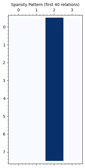
# Visualize the relation matrix structure
# Use the relation matrix from the 20-bit prime with a known factor base

p_vis = 1048583
F_vis = GF(p_vis)
g_vis = F_vis.multiplicative_generator()
S_vis = [2, 3, 5, 7]

c = F_vis(1)
lin_vis = []
for k_val in range(1, 5000):
    c *= g_vis
    complete, li = FactS(ZZ(c), S_vis)
    if complete:
        lin_vis.append([li[q] for q in S_vis] + [k_val])

mm_vis = matrix(ZZ, lin_vis)
A_vis = mm_vis[:, :-1]  # exponent columns only

print(f"Relation matrix: {A_vis.nrows()} relations x {A_vis.ncols()} variables")
print(f"Factor base: {S_vis}")

# Sparsity pattern using matrix_plot
nonzero = matrix(ZZ, [[1 if A_vis[i,j] != 0 else 0
                        for j in range(A_vis.ncols())]
                       for i in range(min(A_vis.nrows(), 40))])
matrix_plot(nonzero, cmap='Blues').show(
    title='Sparsity Pattern (first 40 relations)', figsize=[8, 6])

Relation matrix: 8 relations x 4 variables
Factor base: [2, 3, 5, 7]

# Distribution of nonzero exponent values in the relation matrix
nonzero_vals = [A_vis[i,j] for i in range(A_vis.nrows())
                for j in range(A_vis.ncols()) if A_vis[i,j] > 0]
max_exp = max(nonzero_vals)

from collections import Counter
counts = Counter(nonzero_vals)
bar_data = [(v, counts[v]) for v in sorted(counts.keys())]

bar_chart([c for _, c in bar_data],
          width=0.8,
          color='steelblue').show(
    title='Distribution of Nonzero Exponents in Relation Matrix',
    axes_labels=['Exponent value', 'Frequency'],
    figsize=[8, 5]
)

print(f"Total nonzero entries: {len(nonzero_vals)}")
print(f"Max exponent: {max_exp}")
print("Small primes (2, 3) appear more frequently because smooth numbers")
print("are dominated by small prime factors.")

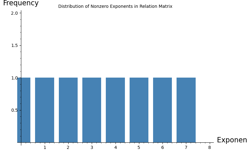
Total nonzero entries: 8
Max exponent: 8
Small primes (2, 3) appear more frequently because smooth numbers
are dominated by small prime factors.

30.9 Experiment 5: Complexity Comparison

# Brute-force DLP solver
def brute_force_log(g, h, p):
    """Solve g^x = h mod p by exhaustive search."""
    F = GF(p)
    g, h = F(g), F(h)
    power = F(1)
    for x in range(p - 1):
        if power == h:
            return x
        power *= g
    return None

# Baby-step / Giant-step DLP solver
def bsgs_log(g, h, p):
    """Baby-step/giant-step for discrete log in GF(p)*."""
    F = GF(p)
    g, h = F(g), F(h)
    n = p - 1  # group order
    m = isqrt(n) + 1

    # Baby step: compute g^j for j = 0, ..., m-1
    table = {}
    power = F(1)
    for j in range(m):
        table[power] = j
        power *= g

    # Giant step: g^(-m)
    g_inv_m = g^(-m)
    gamma = h
    for i in range(m):
        if gamma in table:
            return (i * m + table[gamma]) % n
        gamma *= g_inv_m
    return None

# Quick verification
p_small = 1009
g_small = GF(p_small).multiplicative_generator()
x_true = 456
h_small = g_small^x_true

x_bf = brute_force_log(ZZ(g_small), ZZ(h_small), p_small)
x_bs = bsgs_log(ZZ(g_small), ZZ(h_small), p_small)

print(f"p = {p_small}, g = {g_small}, h = g^{x_true} = {h_small}")
print(f"Brute force:  x = {x_bf}")
print(f"BSGS:         x = {x_bs}")
print(f"All correct: {g_small^x_bf == h_small and g_small^x_bs == h_small}")

p = 1009, g = 11, h = g^456 = 185
Brute force:  x = 456
BSGS:         x = 456
All correct: True

# Compare complexity bounds across different prime sizes
order = g.order()
print(f"For p ~ {ZZ(p).nbits()}-bit prime:")
print(f"  Group order: {order}")
print(f"  Naive (brute force) bound: {order}")
print(f"  Baby-step/Giant-step bound: {float(sqrt(order * 1.0)):.0f}")

# L_p[1/2, sqrt(2)] estimate
from sage.functions.log import log
ln_p = float(log(p))
ln_ln_p = float(log(ln_p))
L = exp(sqrt(2.0) * sqrt(ln_p * ln_ln_p))
print(f"  Index calculus L_p[1/2, sqrt(2)] estimate: {float(L):.0f}")

For p ~ 31-bit prime:
  Group order: 1281772339
  Naive (brute force) bound: 1281772339
  Baby-step/Giant-step bound: 35802
  Index calculus L_p[1/2, sqrt(2)] estimate: 80641

Interpreting the Complexity Bounds

For these small primes, BSGS is typically the fastest algorithm due to low constant factors and the \(O(\sqrt{p})\) complexity. Index calculus incurs overhead from relation collection and linear algebra, which only becomes worthwhile for significantly larger primes (hundreds of bits and beyond).

The advantage of index calculus is asymptotic: its subexponential scaling \(L_p[1/2, c]\) eventually dominates the \(O(p^{1/2})\) scaling of BSGS. For cryptographic-size primes (\(\geq 1024\) bits), index calculus-family algorithms (including the number field sieve) are the only feasible attacks.

30.10 Experiment 6: Smoothness Probability

# Estimate the probability that a random element of (Z/pZ)* is B-smooth
def estimate_smoothness_prob(p, B, n_samples=50000):
    """Estimate the probability that a random element of (Z/pZ)* is B-smooth."""
    fb = [q for q in primes_first_n(prime_pi(B))]
    count = 0
    for _ in range(n_samples):
        val = ZZ(randint(1, p - 1))
        smooth, _ = FactS(val, fb)
        if smooth:
            count += 1
    return count / n_samples

def dickman_approx(u):
    """
    Rough approximation of the Dickman rho function rho(u).
    For u >= 1, rho(u) ~ u^(-u) gives the probability that
    a random integer n is n^(1/u)-smooth.
    """
    if u <= 1:
        return 1.0
    return float(u^(-u))

p_smooth = 1048583
bounds_test = [5, 10, 15, 20, 30, 50, 70, 100, 150, 200]
empirical_probs = []
theoretical_probs = []

for B in bounds_test:
    prob = estimate_smoothness_prob(p_smooth, B, n_samples=30000)
    empirical_probs.append(prob)

    u = float(log(p_smooth) / log(max(B, 2)))
    theoretical_probs.append(dickman_approx(u))

    print(f"B={int(B):4d}: empirical prob = {float(prob):.5f}, "
          f"Dickman approx rho({float(u):.2f}) = {float(dickman_approx(u)):.5f}")

B=   5: empirical prob = 0.00050, Dickman approx rho(8.61) = 0.00000
B=  10: empirical prob = 0.00153, Dickman approx rho(6.02) = 0.00002

B=  15: empirical prob = 0.00417, Dickman approx rho(5.12) = 0.00023

B=  20: empirical prob = 0.00920, Dickman approx rho(4.63) = 0.00083

B=  30: empirical prob = 0.01380, Dickman approx rho(4.08) = 0.00326

B=  50: empirical prob = 0.03160, Dickman approx rho(3.54) = 0.01130

B=  70: empirical prob = 0.04770, Dickman approx rho(3.26) = 0.02109

B= 100: empirical prob = 0.06863, Dickman approx rho(3.01) = 0.03624

B= 150: empirical prob = 0.10923, Dickman approx rho(2.77) = 0.05987

B= 200: empirical prob = 0.13990, Dickman approx rho(2.62) = 0.08073

# Plot smoothness probability: empirical vs Dickman approximation
p_empirical = list_plot(
    list(zip(bounds_test, empirical_probs)),
    plotjoined=True,
    marker='o',
    color='blue',
    scale='semilogy',
    legend_label='Empirical probability'
)

p_dickman = list_plot(
    list(zip(bounds_test, theoretical_probs)),
    plotjoined=True,
    linestyle='--',
    color='red',
    scale='semilogy',
    legend_label=r'Dickman $\rho(u) \approx u^{-u}$'
)

(p_empirical + p_dickman).show(
    title=f'Smoothness Probability for p = {p_smooth} (~20 bits)',
    axes_labels=['Smoothness bound $B$', 'Probability of $B$-smoothness'],
    figsize=[10, 6]
)

The Dickman Function

The probability that a random integer \(n\) is \(n^{1/u}\)-smooth is given by the Dickman rho function \(\rho(u)\). For \(u = \ln p / \ln B\), the smoothness probability of random elements modulo \(p\) is approximately \(\rho(u)\). The crude approximation \(\rho(u) \approx u^{-u}\) already captures the qualitative behavior: smoothness probability decreases rapidly as the ratio \(\ln p / \ln B\) grows.

30.11 Experiment 7: SageMath’s Built-in Factorization

# SageMath provides full integer factorization via .factor()
# This is useful for inspecting the structure of group elements

print("Full factorization of g^10000:")
print(ZZ(g^10000).factor())

print("\nFull factorization of some small powers of g:")
for exponent in [10, 50, 100, 500]:
    val = ZZ(g^exponent)
    print(f"  g^{int(exponent):4d} = {int(val):>12d}  ->  {val.factor()}")

Full factorization of g^10000:
7^2 * 2863897

Full factorization of some small powers of g:
  g^  10 =         1024  ->  2^10
  g^  50 =     56671397  ->  56671397
  g^ 100 =     12163039  ->  7 * 257 * 6761
  g^ 500 =     33053641  ->  3329 * 9929

# Find primes near a given value -- useful for choosing test primes
print("Primes near 1281772337:")
print([i for i in range(100) if (1281772337 + i).is_prime()])

Primes near 1281772337:
[2, 24, 32, 42, 62, 80]

30.12 Exercises

---

Exercise 30.1. Let \(p = 1009\) and \(g = 11\) (a generator of \((\mathbb{Z}/1009\mathbb{Z})^*\)). Use the factor base \(\mathcal{B} = \{2, 3, 5, 7\}\) and manually verify that \(g^1 = 11\), \(g^2 = 121\), \(g^3 = 1331 \bmod 1009 = 313\). Which of these powers are \(\mathcal{B}\)-smooth? Write out the corresponding linear relations modulo \(p - 1 = 1008\).

Hint

A number is \(\mathcal{B}\)-smooth if it factors completely over \(\{2, 3, 5, 7\}\). Recall \(121 = 11^2\) which is not \(\mathcal{B}\)-smooth. Check \(g^k \bmod p\) for small \(k\) until you find enough smooth values. Each smooth value \(g^k \equiv 2^{a} 3^{b} 5^{c} 7^{d} \pmod{p}\) gives \(k \equiv a \log_g 2 + b \log_g 3 + c \log_g 5 + d \log_g 7 \pmod{1008}\).

Exercise 30.2. Implement a function smoothness_ratio(p, B, N) that generates \(N\) random integers in \([1, p)\) and returns the fraction that are \(B\)-smooth. Plot the ratio as a function of \(B\) for \(p = 10^6 + 3\) using SageMath’s list_plot. At what value of \(B\) is approximately 10% of integers smooth?

Hint

Use the FactS function from Section 30.3. Generate random values with randint(1, p-1) and test each. Use list_plot with plotjoined=True for visualization. The 10% threshold can be estimated visually from the plot.

Exercise 30.3. The modular Gaussian elimination can fail when the modulus \(m = p - 1\) is composite and a pivot element has no inverse modulo \(m\). Describe a concrete example where this happens (give specific values of \(p\), the factor base, and the relation matrix), and explain how collecting additional relations can help overcome this issue.

Hint

Consider \(p = 13\), so \(m = 12\). The element \(4\) has \(\gcd(4, 12) = 4 \neq 1\), so \(4\) is not invertible mod 12. If a pivot column contains only entries divisible by 4, elimination fails. Extra relations provide alternative rows that may have coprime pivots. Another approach is to work modulo the prime-power factors of \(m\) separately and combine via CRT.

Exercise 30.4. Modify the Index function to count and report the number of smooth values found during the offset search in Phase 3. Run it for several random targets \(h = g^k\) with \(k\) drawn uniformly at random, and report the average offset \(s\) needed. How does this compare with \(1/\Pr[B\text{-smooth}]\)?

Hint

Sequential scanning has the advantage that you can maintain a running product \(c = h \cdot g^i\) by multiplying by \(g\) at each step (avoiding repeated modular exponentiation). The expected offset is roughly the reciprocal of the smoothness probability for the given factor base.

Exercise 30.5. The subexponential complexity \(L_p[1/2, c]\) depends on the constant \(c\). For the basic index calculus with optimal smoothness bound, one has \(c = \sqrt{2}\). Compute \(L_p[1/2, \sqrt{2}]\) numerically for \(p\) of bit-lengths \(64, 128, 256, 512, 1024\). Plot these values on a log scale and compare with \(\sqrt{p}\) (the BSGS complexity) and \(p\) (brute-force complexity). At what bit-length does index calculus become faster than BSGS according to this estimate?

Hint

Use the formula \(L_p[1/2, c] = \exp(c \sqrt{\ln p \cdot \ln \ln p})\). For \(p \approx 2^n\), \(\ln p \approx n \ln 2\) and \(\ln \ln p \approx \ln(n \ln 2)\). Use SageMath’s list_plot with scale='semilogy' to compare the three complexities.

30.13 Summary and References

---

In this chapter we studied the index calculus algorithm, the first subexponential method for the discrete logarithm problem in prime fields.

Key ideas:

• The algorithm exploits the lifting of group elements to the integers, where factorization provides additional algebraic structure unavailable to generic group algorithms.

• A factor base of small primes defines the notion of smoothness. Smooth powers of the generator yield linear relations among the discrete logarithms of the factor base elements.

• Linear algebra over the integers (using SageMath’s matrix(ZZ, ...), echelon_form(), left_kernel(), and module operations) solves for the base logarithms; individual logarithms follow by expressing the target as a smooth product.

• The smoothness bound \(B\) creates a trade-off: larger \(B\) makes smooth numbers more common but increases the linear system size. The optimal balance gives the celebrated \(L_p[1/2, c]\) complexity.

Historical significance:

• Adleman’s 1979 algorithm was the first to break the \(O(\sqrt{p})\) barrier for DLP in prime fields.

• It inspired a long line of improvements: the Coppersmith-Odlyzko-Schroeppel (COS) algorithm (1986), the Gaussian integer method, and ultimately the number field sieve for DLP, which achieves \(L_p[1/3, c]\) complexity.

• These algorithms are the reason that Diffie-Hellman and ElGamal over \((\mathbb{Z}/p\mathbb{Z})^*\) require primes of at least 2048 bits for modern security.

References:

1. L. M. Adleman, “A subexponential algorithm for the discrete logarithm problem with applications to cryptography,” Proceedings of the 20th Annual IEEE Symposium on Foundations of Computer Science (FOCS), pp. 55–60, 1979.

2. A. M. Odlyzko, “Discrete logarithms: The past and the future,” Designs, Codes and Cryptography, vol. 19, pp. 129–145, 2000.

3. D. Coppersmith, A. M. Odlyzko, and R. Schroeppel, “Discrete logarithms in \(GF(p)\),” Algorithmica, vol. 1, pp. 1–15, 1986.

4. A. J. Menezes, P. C. van Oorschot, and S. A. Vanstone, Handbook of Applied Cryptography, CRC Press, 1996. Chapter 3: Number-Theoretic Reference Problems.