
Chapter 31: Elliptic Curves and the Group Law#
31.1 Historical Background#
The application of elliptic curves to cryptography emerged from two independent proposals in the mid-1980s:
In 1985, Victor Miller presented the idea of using the group of rational points on an elliptic curve over a finite field as the basis for a public-key cryptosystem at a crypto conference, with the paper appearing in 1986.
In 1987, Neal Koblitz independently proposed essentially the same idea, publishing in Mathematics of Computation.
Both recognized a key insight: the discrete logarithm problem on an elliptic curve group appeared to be significantly harder than the corresponding problem in the multiplicative group of a finite field. This meant that the same level of security could be achieved with dramatically smaller key sizes. For example, a 256-bit elliptic curve key provides roughly the same security as a 3072-bit RSA key.
Elliptic curves had been studied as abstract mathematical objects for over a century – by Weierstrass, Mordell, Weil, and many others – but their application to practical cryptography was revolutionary. Today, Elliptic Curve Cryptography (ECC) underpins TLS 1.3, Bitcoin, Signal, and numerous other protocols.
Note
This chapter focuses on the mathematics of elliptic curves: defining the group law, implementing arithmetic over finite fields, and verifying the group axioms computationally. Cryptographic protocols built on these foundations (ECDH, ECDSA, etc.) are treated in later chapters.
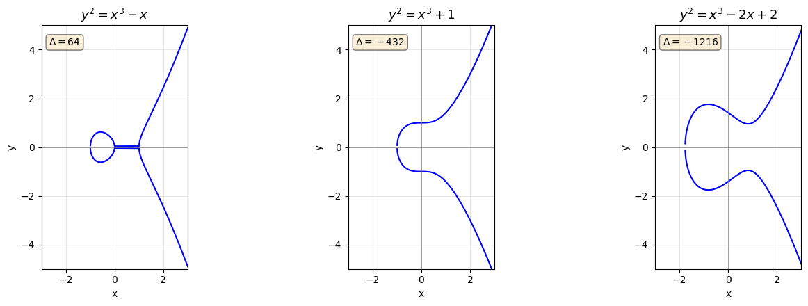
31.2 The Weierstrass Equation#
The discriminant condition \(\Delta \neq 0\) ensures the cubic \(x^3 + ax + b\) has no repeated roots, which is equivalent to the curve having no cusps or self-intersections. When \(\Delta = 0\), the curve degenerates into a singular curve that does not carry a group structure in the usual sense.
Over the real numbers \(\mathbb{R}\), elliptic curves appear as smooth plane curves. Over a finite field \(\mathbb{F}_p\), the “curve” is a discrete set of points. In both cases, the same algebraic formulas define the group operation.
Show code cell source
import numpy as np
import matplotlib.pyplot as plt

# Plot y^2 = x^3 + ax + b over the reals for several parameter choices
fig, axes = plt.subplots(1, 3, figsize=(14, 4.5))

curves = [
    (-1, 0, r"$y^2 = x^3 - x$"),
    (0, 1, r"$y^2 = x^3 + 1$"),
    (-2, 2, r"$y^2 = x^3 - 2x + 2$"),
]

for ax, (a, b, title) in zip(axes, curves):
    x_vals = np.linspace(-3, 3, 2000)
    rhs = x_vals**3 + a * x_vals + b
    # Only plot where rhs >= 0
    mask = rhs >= 0
    y_pos = np.sqrt(rhs[mask])
    y_neg = -y_pos

    ax.plot(x_vals[mask], y_pos, "b-", linewidth=1.5)
    ax.plot(x_vals[mask], y_neg, "b-", linewidth=1.5)
    ax.axhline(0, color="gray", linewidth=0.5)
    ax.axvline(0, color="gray", linewidth=0.5)
    ax.set_title(title, fontsize=13)
    ax.set_xlabel("x")
    ax.set_ylabel("y")
    ax.set_xlim(-3, 3)
    ax.set_ylim(-5, 5)
    ax.set_aspect("equal")
    ax.grid(True, alpha=0.3)

    # Check discriminant
    disc = -16 * (4 * a**3 + 27 * b**2)
    ax.text(0.05, 0.95, f"$\\Delta = {disc}$", transform=ax.transAxes,
            fontsize=10, verticalalignment="top",
            bbox=dict(boxstyle="round", facecolor="wheat", alpha=0.5))

plt.tight_layout()
plt.savefig("fig_ch31_real_curves.png", dpi=150, bbox_inches="tight")
plt.show()
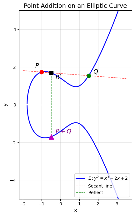
31.3 The Group Law: Point Addition#
The remarkable fact about elliptic curves is that their points form an abelian group under a geometric operation called “point addition.”
Show code cell source
import numpy as np
import matplotlib.pyplot as plt

# Geometric illustration of point addition on y^2 = x^3 - 2x + 2
a, b = -2, 2

fig, ax = plt.subplots(1, 1, figsize=(7, 7))

# Plot the curve
x_vals = np.linspace(-2.0, 3.5, 3000)
rhs = x_vals**3 + a * x_vals + b
mask = rhs >= 0
y_pos = np.sqrt(rhs[mask])
ax.plot(x_vals[mask], y_pos, "b-", linewidth=2, label=r"$E: y^2 = x^3 - 2x + 2$")
ax.plot(x_vals[mask], -y_pos, "b-", linewidth=2)

# Choose two points on the curve
x1 = -1.0
y1 = np.sqrt(x1**3 + a * x1 + b)
x2 = 1.5
y2 = np.sqrt(x2**3 + a * x2 + b)

# Compute the addition
lam = (y2 - y1) / (x2 - x1)
x3 = lam**2 - x1 - x2
y3_intersect = lam * (x1 - x3) - y1  # this is y3 = y-coordinate of P+Q
y3_third = -y3_intersect  # the third intersection point (before reflection)

# Draw the secant line through P and Q
x_line = np.linspace(-2, 3.5, 500)
y_line = lam * (x_line - x1) + y1
ax.plot(x_line, y_line, "r--", linewidth=1.2, alpha=0.7, label="Secant line")

# Draw the vertical reflection line
ax.plot([x3, x3], [y3_third, y3_intersect], "g--", linewidth=1.2, alpha=0.7, label="Reflect")

# Plot points
ax.plot(x1, y1, "ro", markersize=9, zorder=5)
ax.annotate("$P$", (x1, y1), textcoords="offset points", xytext=(-15, 10),
            fontsize=14, fontweight="bold")

ax.plot(x2, y2, "go", markersize=9, zorder=5)
ax.annotate("$Q$", (x2, y2), textcoords="offset points", xytext=(10, 5),
            fontsize=14, fontweight="bold")

ax.plot(x3, y3_third, "ks", markersize=8, zorder=5)
ax.annotate("$R'$", (x3, y3_third), textcoords="offset points", xytext=(10, -15),
            fontsize=13)

ax.plot(x3, y3_intersect, "m^", markersize=11, zorder=5)
ax.annotate("$P+Q$", (x3, y3_intersect), textcoords="offset points", xytext=(10, 8),
            fontsize=14, fontweight="bold", color="purple")

ax.axhline(0, color="gray", linewidth=0.5)
ax.set_xlim(-2.2, 3.8)
ax.set_ylim(-5, 5)
ax.set_aspect("equal")
ax.set_xlabel("x", fontsize=12)
ax.set_ylabel("y", fontsize=12)
ax.set_title("Point Addition on an Elliptic Curve", fontsize=14)
ax.legend(loc="lower right", fontsize=10)
ax.grid(True, alpha=0.3)

plt.tight_layout()
plt.savefig("fig_ch31_point_addition_geometry.png", dpi=150, bbox_inches="tight")
plt.show()

print(f"P = ({float(x1):.4f}, {float(y1):.4f})")
print(f"Q = ({float(x2):.4f}, {float(y2):.4f})")
print(f"P + Q = ({float(x3):.4f}, {float(y3_intersect):.4f})")
P = (-1.0000, 1.7321)
Q = (1.5000, 1.5411)
P + Q = (-0.4942, -1.6934)
31.4 The Group Structure#
Closure and commutativity are relatively straightforward from the addition formulas. The identity and inverse properties follow from the definitions. Associativity is the hardest to prove – it requires a careful algebraic verification (or an argument via the Riemann-Roch theorem). We will verify it computationally in Section 31.7.
31.5 Elliptic Curves over Finite Fields#
When we work over a finite field \(\mathbb{F}_p\) (where \(p > 3\) is prime), all arithmetic is performed modulo \(p\). The curve equation becomes:
and the set of points \(E(\mathbb{F}_p)\) is finite. The following theorem gives a tight bound on how many points the curve can have.
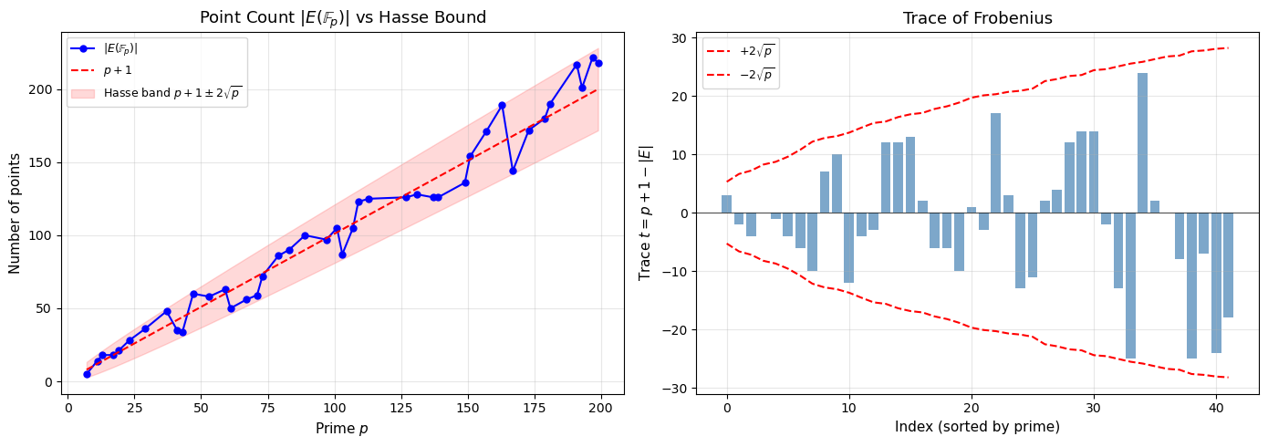
In other words, the number of points is approximately \(p + 1\), with an error of at most \(2\sqrt{p}\). The quantity \(t = p + 1 - \#E(\mathbb{F}_p)\) is called the trace of Frobenius.
Tip
Hasse’s theorem tells us that for large \(p\), the group \(E(\mathbb{F}_p)\) has roughly \(p\) elements. This is crucial for cryptographic applications: if we choose \(p \approx 2^{256}\), the group has approximately \(2^{256}\) elements, making brute-force attacks infeasible.
31.6 Implementation: The EllipticCurve Class#
We now implement a complete elliptic curve arithmetic class over \(\mathbb{F}_p\) using only Python integers and modular arithmetic. Points are represented as (x, y) tuples, with None representing the point at infinity \(\mathcal{O}\).
import numpy as np
import math


class EllipticCurve:
    """Elliptic curve y^2 = x^3 + ax + b over F_p.

    Points are represented as (x, y) tuples with integer coordinates
    in the range [0, p-1]. The point at infinity is represented as None.
    """

    def __init__(self, a, b, p):
        """Initialize the curve E: y^2 = x^3 + ax + b (mod p).

        Parameters
        ----------
        a, b : int
            Curve coefficients.
        p : int
            A prime defining the field F_p.

        Raises
        ------
        ValueError
            If the discriminant is zero (singular curve) or p < 5.
        """
        if p < 5:
            raise ValueError(f"Prime p={p} must be >= 5.")
        self.a = a % p
        self.b = b % p
        self.p = p
        disc = (4 * pow(self.a, 3, p) + 27 * pow(self.b, 2, p)) % p
        if disc == 0:
            raise ValueError(
                f"Singular curve: 4a^3 + 27b^2 = 0 (mod {p}). "
                f"a={self.a}, b={self.b}."
            )

    def is_on_curve(self, P):
        """Check whether P lies on the curve."""
        if P is None:
            return True
        x, y = P
        return (y * y - x * x * x - self.a * x - self.b) % self.p == 0

    def neg(self, P):
        """Return -P."""
        if P is None:
            return None
        x, y = P
        return (x, (-y) % self.p)

    def add(self, P, Q):
        """Return P + Q on the curve."""
        if P is None:
            return Q
        if Q is None:
            return P
        x1, y1 = P
        x2, y2 = Q
        if x1 == x2:
            if (y1 + y2) % self.p == 0:
                # P + (-P) = O
                return None
            else:
                # P == Q, use doubling
                return self.double(P)

        # General addition
        dx = (x2 - x1) % self.p
        dy = (y2 - y1) % self.p
        lam = (dy * pow(dx, -1, self.p)) % self.p
        x3 = (lam * lam - x1 - x2) % self.p
        y3 = (lam * (x1 - x3) - y1) % self.p
        return (x3, y3)

    def double(self, P):
        """Return 2P on the curve."""
        if P is None:
            return None
        x, y = P
        if y == 0:
            return None
        num = (3 * x * x + self.a) % self.p
        den = (2 * y) % self.p
        lam = (num * pow(den, -1, self.p)) % self.p
        x3 = (lam * lam - 2 * x) % self.p
        y3 = (lam * (x - x3) - y) % self.p
        return (x3, y3)

    def scalar_mult(self, k, P):
        """Return k*P using the double-and-add algorithm.

        Parameters
        ----------
        k : int
            Scalar (may be negative).
        P : tuple or None
            A point on the curve.

        Returns
        -------
        tuple or None
            The point k*P.
        """
        if k < 0:
            return self.scalar_mult(-k, self.neg(P))
        if k == 0 or P is None:
            return None
        result = None  # identity
        addend = P
        while k > 0:
            if k & 1:
                result = self.add(result, addend)
            addend = self.double(addend)
            k >>= 1
        return result

    def points(self):
        """Enumerate all points on E(F_p), including O."""
        pts = [None]  # point at infinity
        for x in range(self.p):
            rhs = (x * x * x + self.a * x + self.b) % self.p
            if rhs == 0:
                pts.append((x, 0))
            else:
                # Euler criterion: rhs^((p-1)/2) == 1 mod p iff QR
                if pow(rhs, (self.p - 1) // 2, self.p) == 1:
                    y = self._sqrt_mod(rhs)
                    pts.append((x, y))
                    if y != 0:
                        pts.append((x, self.p - y))
        return pts

    def _sqrt_mod(self, n):
        """Compute a square root of n mod p (Tonelli-Shanks)."""
        p = self.p
        n = n % p
        if n == 0:
            return 0
        if p % 4 == 3:
            return pow(n, (p + 1) // 4, p)
        # Tonelli-Shanks for general primes
        q, s = p - 1, 0
        while q % 2 == 0:
            q //= 2
            s += 1
        z = 2
        while pow(z, (p - 1) // 2, p) != p - 1:
            z += 1
        m, c, t, r = s, pow(z, q, p), pow(n, q, p), pow(n, (q + 1) // 2, p)
        while True:
            if t == 1:
                return r
            i = 1
            tmp = (t * t) % p
            while tmp != 1:
                tmp = (tmp * tmp) % p
                i += 1
            b_val = pow(c, 1 << (m - i - 1), p)
            m, c, t, r = i, (b_val * b_val) % p, (t * b_val * b_val) % p, (r * b_val) % p

    def order(self):
        """Return #E(F_p) by brute-force point counting."""
        return len(self.points())

    def __repr__(self):
        return f"EllipticCurve(a={self.a}, b={self.b}, p={self.p})"


# Quick test
E = EllipticCurve(a=2, b=3, p=97)
print(E)
pts = E.points()
print(f"#E(F_97) = {len(pts)}  (including point at infinity)")
print(f"First 10 affine points: {pts[1:11]}")
EllipticCurve(a=2, b=3, p=97)
#E(F_97) = 100  (including point at infinity)
First 10 affine points: [(0, 87), (0, 10), (1, 54), (1, 43), (3, 91), (3, 6), (4, 47), (4, 50), (10, 76), (10, 21)]
31.7 Verifying Curve Membership#
Let us confirm that every point returned by points() actually satisfies the curve equation \(y^2 \equiv x^3 + ax + b \pmod{p}\).
import numpy as np

# Verify every point is actually on the curve
E = EllipticCurve(a=2, b=3, p=97)
pts = E.points()

all_valid = all(E.is_on_curve(P) for P in pts)
print(f"All {len(pts)} points satisfy the curve equation: {all_valid}")

# Show a few points with verification
print(f"\nSample verifications on E: y^2 = x^3 + {E.a}x + {E.b} (mod {E.p}):")
for P in pts[1:8]:
    x, y = P
    lhs = (y * y) % E.p
    rhs = (x**3 + E.a * x + E.b) % E.p
    print(f"  P = ({int(x):2d}, {int(y):2d})  |  y^2 mod 97 = {int(lhs):2d}  |  "
          f"x^3+2x+3 mod 97 = {int(rhs):2d}  |  match: {lhs == rhs}")
All 100 points satisfy the curve equation: True

Sample verifications on E: y^2 = x^3 + 2x + 3 (mod 97):
  P = ( 0, 87)  |  y^2 mod 97 =  3  |  x^3+2x+3 mod 97 =  3  |  match: True
  P = ( 0, 10)  |  y^2 mod 97 =  3  |  x^3+2x+3 mod 97 =  3  |  match: True
  P = ( 1, 54)  |  y^2 mod 97 =  6  |  x^3+2x+3 mod 97 =  6  |  match: True
  P = ( 1, 43)  |  y^2 mod 97 =  6  |  x^3+2x+3 mod 97 =  6  |  match: True
  P = ( 3, 91)  |  y^2 mod 97 = 36  |  x^3+2x+3 mod 97 = 36  |  match: True
  P = ( 3,  6)  |  y^2 mod 97 = 36  |  x^3+2x+3 mod 97 = 36  |  match: True
  P = ( 4, 47)  |  y^2 mod 97 = 75  |  x^3+2x+3 mod 97 = 75  |  match: True
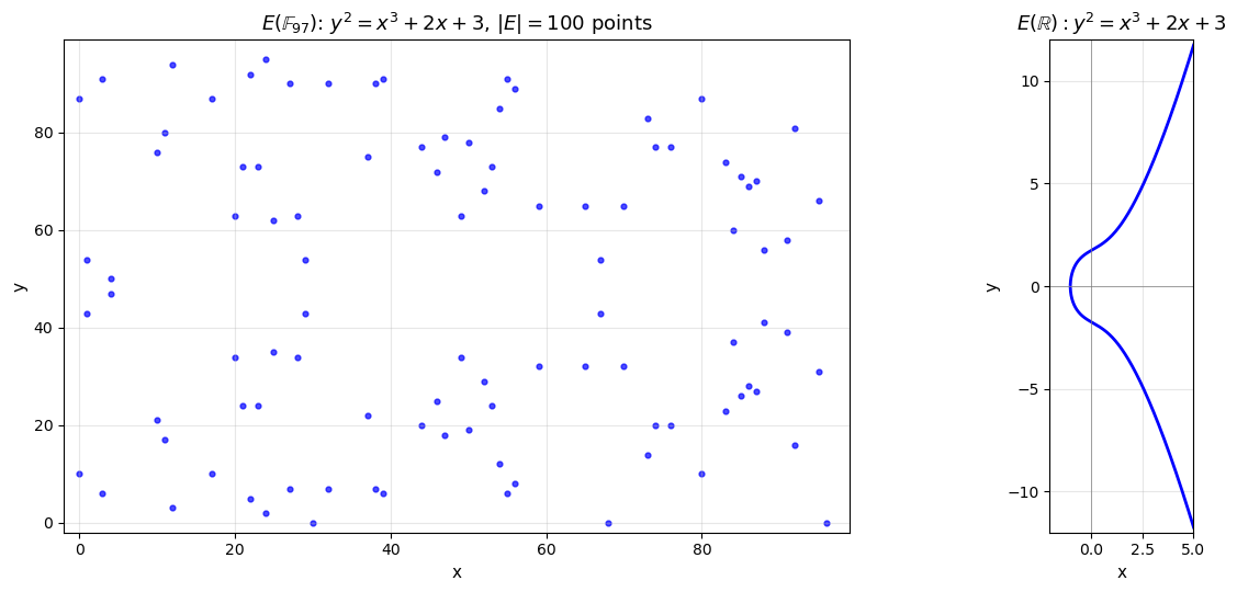
31.8 Plotting the Curve over \(\mathbb{F}_p\) and \(\mathbb{R}\)#
Over the reals, \(E\) is a smooth plane curve. Over \(\mathbb{F}_p\), it becomes a discrete scatter of points. Let us compare the two views for the same curve parameters.
Show code cell source
import numpy as np
import matplotlib.pyplot as plt

# Plot E(F_p) as a discrete scatter plot alongside E(R)
E = EllipticCurve(a=2, b=3, p=97)
pts = E.points()

affine_pts = [P for P in pts if P is not None]
xs = [P[0] for P in affine_pts]
ys = [P[1] for P in affine_pts]

fig, axes = plt.subplots(1, 2, figsize=(14, 5.5))

# Left: F_p scatter
ax = axes[0]
ax.scatter(xs, ys, s=12, c="blue", alpha=0.7)
ax.set_title(f"$E(\\mathbb{{F}}_{{97}})$: $y^2 = x^3 + 2x + 3$, $|E| = {len(pts)}$ points", fontsize=13)
ax.set_xlabel("x", fontsize=11)
ax.set_ylabel("y", fontsize=11)
ax.set_xlim(-2, 99)
ax.set_ylim(-2, 99)
ax.grid(True, alpha=0.3)

# Right: same curve over R for comparison
ax = axes[1]
a_coeff, b_coeff = 2, 3
x_vals = np.linspace(-2, 5, 3000)
rhs = x_vals**3 + a_coeff * x_vals + b_coeff
mask = rhs >= 0
y_pos = np.sqrt(rhs[mask])
ax.plot(x_vals[mask], y_pos, "b-", linewidth=2)
ax.plot(x_vals[mask], -y_pos, "b-", linewidth=2)
ax.axhline(0, color="gray", linewidth=0.5)
ax.axvline(0, color="gray", linewidth=0.5)
ax.set_title(r"$E(\mathbb{R}): y^2 = x^3 + 2x + 3$", fontsize=13)
ax.set_xlabel("x", fontsize=11)
ax.set_ylabel("y", fontsize=11)
ax.set_xlim(-2, 5)
ax.set_ylim(-12, 12)
ax.set_aspect("equal")
ax.grid(True, alpha=0.3)

plt.tight_layout()
plt.savefig("fig_ch31_curve_Fp_vs_R.png", dpi=150, bbox_inches="tight")
plt.show()
31.9 Step-by-Step Point Addition over \(\mathbb{F}_p\)#
Let us pick two points on \(E(\mathbb{F}_{97})\) and trace the addition algorithm step by step, verifying that the result lies on the curve.
import numpy as np

E = EllipticCurve(a=2, b=3, p=97)
pts = E.points()

# Pick two distinct affine points
P = pts[1]
Q = pts[5]
print(f"Curve: y^2 = x^3 + {E.a}x + {E.b} (mod {E.p})")
print(f"P = {P}")
print(f"Q = {Q}")

# Step-by-step addition
x1, y1 = P
x2, y2 = Q
p = E.p

dx = (x2 - x1) % p
dy = (y2 - y1) % p
dx_inv = pow(dx, -1, p)
lam = (dy * dx_inv) % p
x3 = (lam * lam - x1 - x2) % p
y3 = (lam * (x1 - x3) - y1) % p
R = (x3, y3)

print(f"\nStep-by-step:")
print(f"  dx = (x2 - x1) mod {p} = ({x2} - {x1}) mod {p} = {dx}")
print(f"  dy = (y2 - y1) mod {p} = ({y2} - {y1}) mod {p} = {dy}")
print(f"  dx^(-1) mod {p} = {dx_inv}")
print(f"  lambda = dy * dx^(-1) mod {p} = {lam}")
print(f"  x3 = lambda^2 - x1 - x2 mod {p} = {x3}")
print(f"  y3 = lambda*(x1 - x3) - y1 mod {p} = {y3}")
print(f"  P + Q = {R}")
print(f"  On curve? {E.is_on_curve(R)}")

# Verify with the class method
R_class = E.add(P, Q)
print(f"\nUsing E.add: {R_class}")
print(f"Results match: {R == R_class}")
Curve: y^2 = x^3 + 2x + 3 (mod 97)
P = (0, 87)
Q = (3, 91)

Step-by-step:
  dx = (x2 - x1) mod 97 = (3 - 0) mod 97 = 3
  dy = (y2 - y1) mod 97 = (91 - 87) mod 97 = 4
  dx^(-1) mod 97 = 65
  lambda = dy * dx^(-1) mod 97 = 66
  x3 = lambda^2 - x1 - x2 mod 97 = 85
  y3 = lambda*(x1 - x3) - y1 mod 97 = 26
  P + Q = (85, 26)
  On curve? True

Using E.add: (85, 26)
Results match: True
31.10 Verifying the Group Axioms#
We now computationally verify all five group axioms on a small curve \(E(\mathbb{F}_p)\). For a small prime, we can exhaustively check associativity for all triples – a luxury we will not have for cryptographic-size primes.
import numpy as np

# Use a smaller prime for exhaustive verification
E = EllipticCurve(a=1, b=6, p=11)
pts = E.points()
n = len(pts)
print(f"Curve: y^2 = x^3 + x + 6 (mod 11)")
print(f"#E(F_11) = {n}")
print(f"Points: {pts}")

# 1. CLOSURE: P + Q is on the curve for all P, Q
closure_ok = True
for P in pts:
    for Q in pts:
        R = E.add(P, Q)
        if not E.is_on_curve(R):
            closure_ok = False
            print(f"  CLOSURE FAIL: {P} + {Q} = {R}")
print(f"\n1. Closure: {'PASS' if closure_ok else 'FAIL'}")

# 2. IDENTITY: P + O = P for all P
identity_ok = all(E.add(P, None) == P and E.add(None, P) == P for P in pts)
print(f"2. Identity (O): {'PASS' if identity_ok else 'FAIL'}")

# 3. INVERSES: P + (-P) = O for all P
inverse_ok = all(E.add(P, E.neg(P)) is None for P in pts)
print(f"3. Inverses: {'PASS' if inverse_ok else 'FAIL'}")

# 4. COMMUTATIVITY: P + Q = Q + P for all P, Q
comm_ok = True
for P in pts:
    for Q in pts:
        if E.add(P, Q) != E.add(Q, P):
            comm_ok = False
print(f"4. Commutativity: {'PASS' if comm_ok else 'FAIL'}")

# 5. ASSOCIATIVITY: (P + Q) + R = P + (Q + R) for all P, Q, R
assoc_ok = True
count = 0
for P in pts:
    for Q in pts:
        for R in pts:
            lhs = E.add(E.add(P, Q), R)
            rhs = E.add(P, E.add(Q, R))
            if lhs != rhs:
                assoc_ok = False
                print(f"  ASSOC FAIL: P={P}, Q={Q}, R={R}")
            count += 1
print(f"5. Associativity: {'PASS' if assoc_ok else 'FAIL'}  ({count} triples checked)")
Curve: y^2 = x^3 + x + 6 (mod 11)
#E(F_11) = 13
Points: [None, (2, 4), (2, 7), (3, 5), (3, 6), (5, 9), (5, 2), (7, 9), (7, 2), (8, 3), (8, 8), (10, 9), (10, 2)]

1. Closure: PASS
2. Identity (O): PASS
3. Inverses: PASS
4. Commutativity: PASS
5. Associativity: PASS  (2197 triples checked)
31.11 Scalar Multiplication and the Double-and-Add Algorithm#
Given a point \(P\) and a positive integer \(k\), the scalar multiple \(kP\) is defined as:
Computing this naively requires \(k - 1\) additions, which is infeasible when \(k \approx 2^{256}\). The double-and-add algorithm (analogous to square-and-multiply for modular exponentiation) computes \(kP\) in \(O(\log k)\) group operations by processing the binary representation of \(k\).
import numpy as np

E = EllipticCurve(a=2, b=3, p=97)
pts = E.points()
P = pts[1]

print(f"Curve: y^2 = x^3 + {E.a}x + {E.b} (mod {E.p})")
print(f"Base point P = {P}")
print(f"\nScalar multiples of P:")
print(f"{'k':>4s}  {'kP':>20s}  {'on curve?':>10s}")
print("-" * 40)

# Compute successive multiples
for k in range(1, 20):
    kP = E.scalar_mult(k, P)
    on_curve = E.is_on_curve(kP)
    if kP is None:
        print(f"{int(k):4d}  {'O (infinity)':>20s}  {str(on_curve):>10s}")
    else:
        print(f"{int(k):4d}  {str(kP):>20s}  {str(on_curve):>10s}")

# Find the order of P (smallest k > 0 with kP = O)
order_P = None
for k in range(1, len(pts) + 1):
    if E.scalar_mult(k, P) is None:
        order_P = k
        break
print(f"\nOrder of P: {order_P}")
print(f"#E(F_{E.p}) = {len(pts)}")
print(f"Order of P divides #E? {len(pts) % order_P == 0}")
Curve: y^2 = x^3 + 2x + 3 (mod 97)
Base point P = (0, 87)

Scalar multiples of P:
   k                    kP   on curve?
----------------------------------------
   1               (0, 87)        True
   2              (65, 65)        True
   3              (23, 73)        True
   4              (52, 29)        True
   5              (88, 41)        True
   6              (95, 31)        True
   7              (10, 21)        True
   8              (84, 60)        True
   9              (11, 17)        True
  10              (80, 87)        True
  11              (17, 10)        True
  12              (74, 77)        True
  13              (87, 27)        True
  14              (46, 25)        True
  15              (53, 73)        True
  16              (92, 16)        True
  17               (1, 54)        True
  18              (21, 24)        True
  19              (85, 71)        True

Order of P: 50
#E(F_97) = 100
Order of P divides #E? True
31.12 Tracing the Double-and-Add Algorithm#
The double-and-add method processes the binary digits of \(k\) from the least significant bit to the most. Here we trace each step to see how \(kP\) is built up.
import numpy as np

E = EllipticCurve(a=2, b=3, p=97)
pts = E.points()
P = pts[1]

k = 53
print(f"Computing {k} * P where P = {P}")
print(f"Binary representation of {k}: {bin(k)}")
print(f"Binary digits (MSB first): {[int(b) for b in bin(k)[2:]]}")
print()

# Trace the right-to-left double-and-add
result = None
addend = P
k_copy = k
step = 0

print(f"{'Step':>4s}  {'Bit':>3s}  {'Action':>15s}  {'Result':>25s}  {'Addend':>25s}")
print("-" * 80)

while k_copy > 0:
    bit = k_copy & 1
    if bit:
        result = E.add(result, addend)
        action = "add"
    else:
        action = "skip"

    result_str = str(result) if result is not None else "O"
    addend_str = str(addend) if addend is not None else "O"
    print(f"{int(step):4d}  {int(bit):3d}  {action:>15s}  {result_str:>25s}  {addend_str:>25s}")

    addend = E.double(addend)
    k_copy >>= 1
    step += 1

print(f"\nFinal result: {k}P = {result}")
print(f"Verification: {E.scalar_mult(k, P)}")
print(f"Match: {result == E.scalar_mult(k, P)}")
print(f"\nTotal group operations: {step} doubles + {bin(k).count('1')} adds")
print(f"Naive method would require {k - 1} additions")
Computing 53 * P where P = (0, 87)
Binary representation of 53: 0b110101
Binary digits (MSB first): [1, 1, 0, 1, 0, 1]

Step  Bit           Action                     Result                     Addend
--------------------------------------------------------------------------------
   0    1              add                    (0, 87)                    (0, 87)
   1    0             skip                    (0, 87)                   (65, 65)
   2    1              add                   (88, 41)                   (52, 29)
   3    0             skip                   (88, 41)                   (84, 60)
   4    1              add                   (47, 18)                   (92, 16)
   5    1              add                   (23, 73)                   (21, 73)

Final result: 53P = (23, 73)
Verification: (23, 73)
Match: True

Total group operations: 6 doubles + 4 adds
Naive method would require 52 additions
31.13 The Elliptic Curve Discrete Logarithm Problem (ECDLP)#
The best known algorithms for the general ECDLP on a well-chosen curve run in \(O(\sqrt{n})\) time (e.g., Pollard’s rho algorithm). There is no known sub-exponential algorithm (unlike the ordinary DLP in \(\mathbb{F}_p^*\), which can be solved in sub-exponential time via the number field sieve). This is the fundamental reason ECC can use shorter keys than RSA or classical Diffie-Hellman.
Warning
Not all elliptic curves are suitable for cryptography. Curves susceptible to the MOV attack (embedding degree too small), anomalous curves (\(\#E(\mathbb{F}_p) = p\)), or curves with other special structure can have their ECDLP solved efficiently. Standardized curves (NIST P-256, Curve25519, etc.) are carefully chosen to avoid these pitfalls.
import numpy as np

E = EllipticCurve(a=2, b=3, p=97)
pts = E.points()
n_E = len(pts)

# Find a point with large order to use as a base point
G = None
order_G = 0
for candidate in pts[1:]:
    for k in range(1, n_E + 1):
        if E.scalar_mult(k, candidate) is None:
            if k > order_G:
                order_G = k
                G = candidate
            break
    if order_G == n_E:
        break  # found a generator

print(f"Base point G = {G}, order = {order_G}")

# Choose a secret scalar and compute Q = kG
secret_k = 42
Q = E.scalar_mult(secret_k, G)
print(f"\nSecret k = {secret_k}")
print(f"Public Q = kG = {Q}")

# Brute-force ECDLP
print(f"\nBrute-force search for k such that kG = {Q}:")
for k_test in range(order_G):
    if E.scalar_mult(k_test, G) == Q:
        print(f"  Found: k = {k_test}")
        break

print(f"\nFor a 256-bit curve, brute force requires ~2^256 operations.")
print(f"Pollard's rho requires ~2^128 operations -- still infeasible.")
Base point G = (0, 87), order = 50

Secret k = 42
Public Q = kG = (84, 37)

Brute-force search for k such that kG = (84, 37):
  Found: k = 42

For a 256-bit curve, brute force requires ~2^256 operations.
Pollard's rho requires ~2^128 operations -- still infeasible.
31.14 Verifying Hasse’s Theorem#
We now verify Hasse’s bound \(|\#E(\mathbb{F}_p) - p - 1| \leq 2\sqrt{p}\) by counting points on a fixed curve for several primes, and plotting the results.
Show code cell source
import numpy as np
import matplotlib.pyplot as plt
import math

# Count points on y^2 = x^3 + x + 1 for various primes
primes = [7, 11, 13, 17, 19, 23, 29, 31, 37, 41, 43, 47, 53, 59, 61, 67,
          71, 73, 79, 83, 89, 97, 101, 103, 107, 109, 113, 127, 131, 137,
          139, 149, 151, 157, 163, 167, 173, 179, 181, 191, 193, 197, 199]

a_coeff, b_coeff = 1, 1
valid_primes = []
counts = []
traces = []

for p in primes:
    try:
        E_tmp = EllipticCurve(a_coeff, b_coeff, p)
        n = E_tmp.order()
        valid_primes.append(p)
        counts.append(n)
        traces.append(p + 1 - n)
    except ValueError:
        pass  # singular curve for this prime

ps = np.array(valid_primes)
cs = np.array(counts)
ts = np.array(traces)

fig, axes = plt.subplots(1, 2, figsize=(14, 5))

# Left: point count vs p+1
ax = axes[0]
ax.plot(ps, cs, "bo-", markersize=5, label=r"$|E(\mathbb{F}_p)|$")
ax.plot(ps, ps + 1, "r--", linewidth=1.5, label=r"$p + 1$")
ax.fill_between(ps, ps + 1 - 2*np.sqrt(ps), ps + 1 + 2*np.sqrt(ps),
                alpha=0.15, color="red", label=r"Hasse band $p+1 \pm 2\sqrt{p}$")
ax.set_xlabel("Prime $p$", fontsize=11)
ax.set_ylabel("Number of points", fontsize=11)
ax.set_title(r"Point Count $|E(\mathbb{F}_p)|$ vs Hasse Bound", fontsize=13)
ax.legend(fontsize=9)
ax.grid(True, alpha=0.3)

# Right: trace of Frobenius
ax = axes[1]
ax.bar(range(len(ts)), ts, color="steelblue", alpha=0.7)
ax.axhline(0, color="black", linewidth=0.5)
hasse_bounds = 2 * np.sqrt(ps)
ax.plot(range(len(ts)), hasse_bounds, "r--", label=r"$+2\sqrt{p}$")
ax.plot(range(len(ts)), -hasse_bounds, "r--", label=r"$-2\sqrt{p}$")
ax.set_xlabel("Index (sorted by prime)", fontsize=11)
ax.set_ylabel(r"Trace $t = p + 1 - |E|$", fontsize=11)
ax.set_title("Trace of Frobenius", fontsize=13)
ax.legend(fontsize=9)
ax.grid(True, alpha=0.3)

plt.tight_layout()
plt.savefig("fig_ch31_hasse_bound.png", dpi=150, bbox_inches="tight")
plt.show()

# Print table
print(f"{'p':>5s}  {'#E':>5s}  {'p+1':>5s}  {'trace':>6s}  {'2sqrt(p)':>9s}  {'Hasse OK?':>10s}")
print("-" * 48)
for p_val, c_val, t_val in zip(ps, cs, ts):
    bound = 2 * math.sqrt(p_val)
    ok = abs(t_val) <= bound
    print(f"{int(p_val):5d}  {int(c_val):5d}  {int(p_val+1):5d}  {int(t_val):6d}  {float(bound):9.2f}  {'YES' if ok else 'NO':>10s}")
    p     #E    p+1   trace   2sqrt(p)   Hasse OK?
------------------------------------------------
    7      5      8       3       5.29         YES
   11     14     12      -2       6.63         YES
   13     18     14      -4       7.21         YES
   17     18     18       0       8.25         YES
   19     21     20      -1       8.72         YES
   23     28     24      -4       9.59         YES
   29     36     30      -6      10.77         YES
   37     48     38     -10      12.17         YES
   41     35     42       7      12.81         YES
   43     34     44      10      13.11         YES
   47     60     48     -12      13.71         YES
   53     58     54      -4      14.56         YES
   59     63     60      -3      15.36         YES
   61     50     62      12      15.62         YES
   67     56     68      12      16.37         YES
   71     59     72      13      16.85         YES
   73     72     74       2      17.09         YES
   79     86     80      -6      17.78         YES
   83     90     84      -6      18.22         YES
   89    100     90     -10      18.87         YES
   97     97     98       1      19.70         YES
  101    105    102      -3      20.10         YES
  103     87    104      17      20.30         YES
  107    105    108       3      20.69         YES
  109    123    110     -13      20.88         YES
  113    125    114     -11      21.26         YES
  127    126    128       2      22.54         YES
  131    128    132       4      22.89         YES
  137    126    138      12      23.41         YES
  139    126    140      14      23.58         YES
  149    136    150      14      24.41         YES
  151    154    152      -2      24.58         YES
  157    171    158     -13      25.06         YES
  163    189    164     -25      25.53         YES
  167    144    168      24      25.85         YES
  173    172    174       2      26.31         YES
  179    180    180       0      26.76         YES
  181    190    182      -8      26.91         YES
  191    217    192     -25      27.64         YES
  193    201    194      -7      27.78         YES
  197    222    198     -24      28.07         YES
  199    218    200     -18      28.21         YES
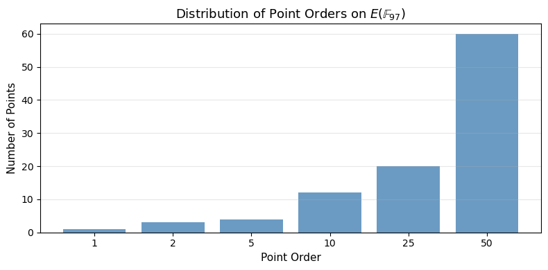
31.15 Group Structure and Point Orders#
The group \(E(\mathbb{F}_p)\) is always isomorphic to \(\mathbb{Z}/n_1\mathbb{Z} \times \mathbb{Z}/n_2\mathbb{Z}\) for some \(n_1, n_2\) with \(n_2 \mid n_1\). In many cases (especially for cryptographic curves), \(n_2 = 1\), meaning the group is cyclic. A point \(G\) whose order equals \(\#E(\mathbb{F}_p)\) is called a generator of the group.
Let us examine the order distribution of points on our curve.
Show code cell source
import numpy as np
import matplotlib.pyplot as plt
from collections import Counter

E = EllipticCurve(a=2, b=3, p=97)
pts = E.points()
n_E = len(pts)

print(f"Curve: y^2 = x^3 + {E.a}x + {E.b} (mod {E.p})")
print(f"#E(F_{E.p}) = {n_E}")

# Compute order of each point
orders = {}
generators = []
for P in pts:
    if P is None:
        orders[str(P)] = 1
        continue
    for k in range(1, n_E + 1):
        if E.scalar_mult(k, P) is None:
            orders[str(P)] = k
            if k == n_E:
                generators.append(P)
            break

# Distribution of orders
order_counts = Counter(orders.values())
print(f"\nOrder distribution:")
for order in sorted(order_counts.keys()):
    print(f"  Order {int(order):4d}: {int(order_counts[order]):3d} points")

print(f"\nNumber of generators (order = {n_E}): {len(generators)}")
if generators:
    print(f"Sample generators: {generators[:5]}")

# Factor the group order
def factorize(n):
    factors = []
    d = 2
    while d * d <= n:
        while n % d == 0:
            factors.append(d)
            n //= d
        d += 1
    if n > 1:
        factors.append(n)
    return factors

print(f"\nFactorization of #E = {n_E}: {factorize(n_E)}")

# Plot order distribution
fig, ax = plt.subplots(figsize=(8, 4))
order_vals = sorted(order_counts.keys())
order_freqs = [order_counts[o] for o in order_vals]
ax.bar([str(o) for o in order_vals], order_freqs, color="steelblue", alpha=0.8)
ax.set_xlabel("Point Order", fontsize=11)
ax.set_ylabel("Number of Points", fontsize=11)
ax.set_title(f"Distribution of Point Orders on $E(\\mathbb{{F}}_{{{E.p}}})$", fontsize=13)
ax.grid(True, alpha=0.3, axis="y")

plt.tight_layout()
plt.savefig("fig_ch31_order_distribution.png", dpi=150, bbox_inches="tight")
plt.show()
Curve: y^2 = x^3 + 2x + 3 (mod 97)
#E(F_97) = 100

Order distribution:
  Order    1:   1 points
  Order    2:   3 points
  Order    5:   4 points
  Order   10:  12 points
  Order   25:  20 points
  Order   50:  60 points

Number of generators (order = 100): 0

Factorization of #E = 100: [2, 2, 5, 5]
31.16 Singular Curves: A Cautionary Note#
When the discriminant \(\Delta = -16(4a^3 + 27b^2)\) vanishes, the curve is singular – it has a cusp or a node. Singular curves do not form a group in the usual sense, and their “discrete logarithm problem” can be solved efficiently. This is why the discriminant check is critical.
Show code cell source
import numpy as np
import matplotlib.pyplot as plt

fig, axes = plt.subplots(1, 2, figsize=(12, 5))

# Cusp: y^2 = x^3 (a=0, b=0, discriminant = 0)
ax = axes[0]
x_vals = np.linspace(-1, 3, 2000)
rhs = x_vals**3
mask = rhs >= 0
y_pos = np.sqrt(rhs[mask])
ax.plot(x_vals[mask], y_pos, "r-", linewidth=2)
ax.plot(x_vals[mask], -y_pos, "r-", linewidth=2)
ax.plot(0, 0, "ko", markersize=8)
ax.annotate("Cusp", (0, 0), textcoords="offset points", xytext=(15, 15),
            fontsize=12, fontweight="bold",
            arrowprops=dict(arrowstyle="->", color="black"))
ax.set_title(r"$y^2 = x^3$ (cusp, $\Delta = 0$)", fontsize=13, color="red")
ax.set_xlim(-1.5, 3)
ax.set_ylim(-4, 4)
ax.set_aspect("equal")
ax.grid(True, alpha=0.3)

# Node: y^2 = (x-1)^2(x+2) has a node at x=1
ax = axes[1]
x_vals = np.linspace(-2.5, 3, 3000)
rhs = (x_vals - 1)**2 * (x_vals + 2)
mask = rhs >= 0
y_pos = np.sqrt(rhs[mask])
ax.plot(x_vals[mask], y_pos, "r-", linewidth=2)
ax.plot(x_vals[mask], -y_pos, "r-", linewidth=2)
ax.plot(1, 0, "ko", markersize=8)
ax.annotate("Node", (1, 0), textcoords="offset points", xytext=(15, 15),
            fontsize=12, fontweight="bold",
            arrowprops=dict(arrowstyle="->", color="black"))
ax.set_title(r"$y^2 = (x-1)^2(x+2)$ (node, $\Delta = 0$)", fontsize=13, color="red")
ax.set_xlim(-2.5, 3)
ax.set_ylim(-4, 4)
ax.set_aspect("equal")
ax.grid(True, alpha=0.3)

plt.tight_layout()
plt.savefig("fig_ch31_singular_curves.png", dpi=150, bbox_inches="tight")
plt.show()

# Show that our class correctly rejects singular curves
for a_test, b_test in [(0, 0), (-3, 2)]:
    try:
        E_bad = EllipticCurve(a_test, b_test, 97)
        print(f"a={a_test}, b={b_test}: accepted (unexpected)")
    except ValueError as e:
        print(f"a={a_test}, b={b_test}: correctly rejected -- {e}")

a=0, b=0: correctly rejected -- Singular curve: 4a^3 + 27b^2 = 0 (mod 97). a=0, b=0.
a=-3, b=2: correctly rejected -- Singular curve: 4a^3 + 27b^2 = 0 (mod 97). a=94, b=2.
31.17 Comparing Curves: Point Counts and the Hasse Band#
Different curve parameters \((a, b)\) yield different group orders over the same field. Let us survey several curves over \(\mathbb{F}_{97}\) and see how their point counts distribute within the Hasse band.
Show code cell source
import numpy as np
import matplotlib.pyplot as plt
import math

p = 97
hasse_center = p + 1

print(f"p = {p}")
print(f"Hasse band: [{float(p + 1 - 2*math.sqrt(p)):.1f}, {float(p + 1 + 2*math.sqrt(p)):.1f}]")
print(f"Center: p + 1 = {hasse_center}")
print()

curve_orders = []

for a in range(0, 10):
    for b in range(1, 10):
        disc = (4 * a**3 + 27 * b**2) % p
        if disc == 0:
            continue
        try:
            E_tmp = EllipticCurve(a, b, p)
            n = E_tmp.order()
            curve_orders.append(n)
        except ValueError:
            continue

curve_orders = np.array(curve_orders)

fig, ax = plt.subplots(figsize=(10, 5))
ax.hist(curve_orders, bins=range(int(curve_orders.min()) - 1, int(curve_orders.max()) + 2),
        color="steelblue", alpha=0.7, edgecolor="white")
ax.axvline(hasse_center, color="red", linestyle="--", linewidth=2,
           label=f"$p+1 = {hasse_center}$")
ax.axvline(hasse_center - 2*math.sqrt(p), color="orange", linestyle=":",
           linewidth=2, label=r"$p+1 - 2\sqrt{p}$")
ax.axvline(hasse_center + 2*math.sqrt(p), color="orange", linestyle=":",
           linewidth=2, label=r"$p+1 + 2\sqrt{p}$")
ax.set_xlabel(r"$|E|(\mathbb{F}_{97})$", fontsize=12)
ax.set_ylabel("Number of curves", fontsize=12)
ax.set_title(f"Distribution of Point Counts for Various Curves over "
             f"$\\mathbb{{F}}_{{{p}}}$", fontsize=13)
ax.legend(fontsize=10)
ax.grid(True, alpha=0.3, axis="y")

plt.tight_layout()
plt.savefig("fig_ch31_order_histogram.png", dpi=150, bbox_inches="tight")
plt.show()

print(f"Total non-singular curves tested: {len(curve_orders)}")
print(f"Min #E = {curve_orders.min()}, Max #E = {curve_orders.max()}")
print(f"All within Hasse bound: "
      f"{all(abs(int(n) - hasse_center) <= 2*math.sqrt(p) for n in curve_orders)}")
p = 97
Hasse band: [78.3, 117.7]
Center: p + 1 = 98
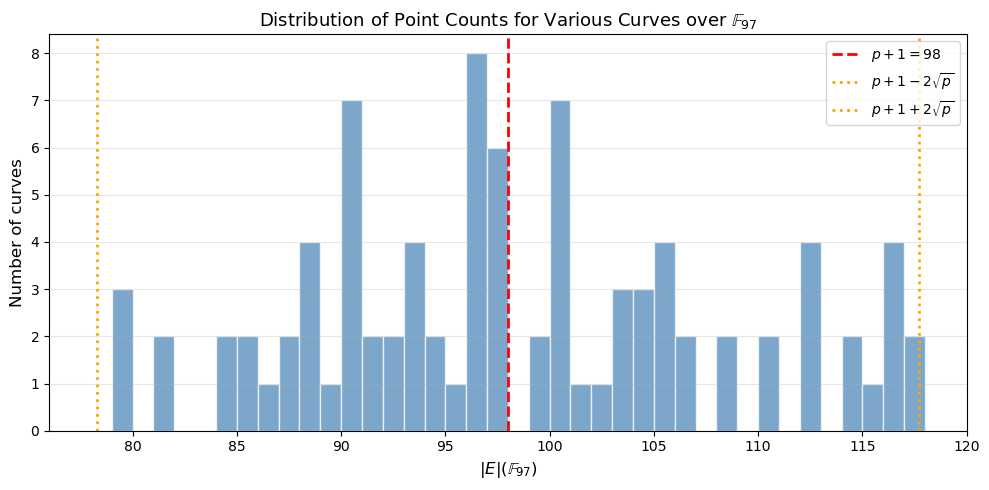
Total non-singular curves tested: 89
Min #E = 79, Max #E = 117
All within Hasse bound: True
31.18 Exercises#
31.19 Summary#
In this chapter we established the mathematical foundations of elliptic curve arithmetic:
An elliptic curve in short Weierstrass form is \(y^2 = x^3 + ax + b\) with \(4a^3 + 27b^2 \neq 0\) (non-singular).
The points on \(E\) over a field \(K\), together with a point at infinity \(\mathcal{O}\), form an abelian group under the chord-and-tangent addition law.
Over a finite field \(\mathbb{F}_p\), Hasse’s theorem constrains the group order: \(|\#E(\mathbb{F}_p) - p - 1| \leq 2\sqrt{p}\).
The scalar multiplication \(kP\) is computed efficiently via the double-and-add algorithm in \(O(\log k)\) group operations.
The Elliptic Curve Discrete Logarithm Problem (ECDLP) – given \(G\) and \(Q = kG\), find \(k\) – is believed to be computationally intractable for well-chosen curves, forming the basis of modern ECC.
We implemented a complete EllipticCurve class over \(\mathbb{F}_p\) and verified all group axioms computationally.
Tip
Looking ahead. In subsequent chapters, we will use the group law developed here to build cryptographic protocols: ECDH (key exchange), ECDSA (digital signatures), and EdDSA (Edwards-curve signatures). We will also study specialized attacks on poorly chosen curves.
31.20 References#
V. S. Miller, “Use of Elliptic Curves in Cryptography,” Advances in Cryptology – CRYPTO ‘85, LNCS 218, Springer, 1986, pp. 417–426.
N. Koblitz, “Elliptic Curve Cryptosystems,” Mathematics of Computation, vol. 48, no. 177, 1987, pp. 203–209.
J. H. Silverman, The Arithmetic of Elliptic Curves, 2nd edition, Graduate Texts in Mathematics 106, Springer, 2009.
L. C. Washington, Elliptic Curves: Number Theory and Cryptography, 2nd edition, CRC Press, 2008.
H. Hasse, “Zur Theorie der abstrakten elliptischen Funktionenkorper,” Journal fur die reine und angewandte Mathematik, 1936.
D. Hankerson, A. Menezes, S. Vanstone, Guide to Elliptic Curve Cryptography, Springer, 2004.