
Chapter 22: Finite Fields and GF(2^8) (SageMath)#
Python Version Available
This notebook contains the SageMath implementation. A pure Python/NumPy version is available in Chapter 22: Finite Field Arithmetic in GF(2^8).
SageMath provides built-in finite field arithmetic via GF(), PolynomialRing(), and quotient ring constructions. Operations that required hundreds of lines of manual Python (shift-and-XOR multiplication, extended GCD for polynomials, inverse tables) become one-liners in SageMath.
22.1 Introduction: Galois Fields and AES#
In 1830, the French mathematician Evariste Galois (1811–1832), in the last years of his tragically short life, laid the foundations of what we now call Galois theory. Among his discoveries was the complete classification of finite fields: for every prime \(p\) and positive integer \(n\), there exists a unique (up to isomorphism) finite field of order \(p^n\), denoted \(\mathrm{GF}(p^n)\) or \(\mathbb{F}_{p^n}\).
The field \(\mathrm{GF}(2^8)\) – a finite field with \(256\) elements – occupies a special place in modern cryptography. When Joan Daemen and Vincent Rijmen designed the Rijndael cipher in 1998 (which became the Advanced Encryption Standard in 2001), they chose \(\mathrm{GF}(2^8)\) as the algebraic foundation for nearly every operation in the cipher.
“The choice of \(\mathrm{GF}(2^8)\) as the basic algebraic structure was motivated by the fact that the elements of this field can be represented as bytes, making efficient software and hardware implementations possible.” – Daemen & Rijmen, The Design of Rijndael, 2002
Why \(\mathrm{GF}(2^8)\) specifically?
Byte representation. Each element of \(\mathrm{GF}(2^8)\) corresponds naturally to a single byte (8 bits), the fundamental unit of computation.
Efficient arithmetic. Addition in \(\mathrm{GF}(2^8)\) is simply XOR, which is one of the fastest operations on any processor.
Rich algebraic structure. Every nonzero element has a multiplicative inverse, enabling the construction of the AES S-box – the nonlinear component critical to the cipher’s security.
Hardware friendliness. Polynomial multiplication and reduction modulo a fixed polynomial can be implemented efficiently in both hardware and software.
The specific field used in AES is \(\mathrm{GF}(2^8)\) defined by the irreducible polynomial \(m(x) = x^8 + x^4 + x^3 + x + 1\) (hexadecimal 0x11B). This polynomial was chosen by the AES designers because it is the lexicographically first degree-8 irreducible polynomial over \(\mathrm{GF}(2)\) and produces an efficient reduction step.
Tip
Understanding \(\mathrm{GF}(2^8)\) arithmetic is essential for understanding AES at a mathematical level. The SubBytes step uses multiplicative inverses in this field, MixColumns uses polynomial multiplication over \(\mathrm{GF}(2^8)\), and AddRoundKey is simply addition (XOR) in the field.
SageMath Advantage
In the Python version of this chapter, we built a complete GF256 class from scratch (~200 lines) implementing shift-and-XOR multiplication, polynomial division, the extended Euclidean algorithm, and lookup tables. In SageMath, all of this is built in. The single line GF(2^8) creates a fully functional finite field with arithmetic, inverses, and group structure immediately available.
22.2 Formal Definitions#
Definition 22.1 (The Binary Field \(\mathrm{GF}(2)\))
The binary field \(\mathrm{GF}(2) = \{0, 1\}\) is the finite field with two elements, where both addition and multiplication are performed modulo 2:
\(+\) |
0 |
1 |
|---|---|---|
0 |
0 |
1 |
1 |
1 |
0 |
\(\cdot\) |
0 |
1 |
|---|---|---|
0 |
0 |
0 |
1 |
0 |
1 |
Note that addition in \(\mathrm{GF}(2)\) is the XOR operation, and subtraction is identical to addition (since \(-1 \equiv 1 \pmod{2}\)).
Definition 22.2 (Polynomial Ring \(\mathrm{GF}(2)[x]\))
The polynomial ring \(\mathrm{GF}(2)[x]\) is the set of all polynomials with coefficients in \(\mathrm{GF}(2)\):
Addition and multiplication follow the usual polynomial rules, with all coefficient arithmetic done modulo 2. For example:
since \(1 + 1 = 0\) in \(\mathrm{GF}(2)\).
Definition 22.3 (The Finite Field \(\mathrm{GF}(2^8)\))
Let \(m(x) = x^8 + x^4 + x^3 + x + 1\) be an irreducible polynomial over \(\mathrm{GF}(2)\) (it has no nontrivial factors in \(\mathrm{GF}(2)[x]\)). The finite field \(\mathrm{GF}(2^8)\) is the quotient ring:
Its elements are the 256 polynomials of degree \(< 8\) over \(\mathrm{GF}(2)\):
Each element corresponds to a byte \((a_7, a_6, \ldots, a_1, a_0)\), or equivalently an integer in \(\{0, 1, \ldots, 255\}\).
Definition 22.4 (Addition in \(\mathrm{GF}(2^8)\))
Addition in \(\mathrm{GF}(2^8)\) is coefficient-wise addition modulo 2, which is equivalent to the bitwise XOR operation:
For example, 0x57 \(+\) 0x83 \(=\) 0xD4, since \(01010111 \oplus 10000011 = 11010100\).
Definition 22.5 (Multiplication in \(\mathrm{GF}(2^8)\))
Multiplication in \(\mathrm{GF}(2^8)\) is polynomial multiplication followed by reduction modulo \(m(x)\):
The reduction ensures the result is a polynomial of degree \(\leq 7\) (a single byte). For example, \(\{57\} \cdot \{83\} = \{\mathrm{C1}\}\) in the AES field.
Definition 22.6 (Multiplicative Inverse via Extended Euclidean Algorithm)
For a nonzero element \(a(x) \in \mathrm{GF}(2^8)\), its multiplicative inverse \(a^{-1}(x)\) satisfies:
It is computed using the extended Euclidean algorithm for polynomials over \(\mathrm{GF}(2)\). Since \(m(x)\) is irreducible and \(\deg(a) < \deg(m)\), we have \(\gcd(a(x), m(x)) = 1\), so Bezout’s identity gives:
and \(a^{-1}(x) = s(x) \mod m(x)\).
Theorem 22.1 (Existence of Multiplicative Inverses)
Every nonzero element of \(\mathrm{GF}(2^8)\) has a unique multiplicative inverse. Equivalently, \((\mathrm{GF}(2^8) \setminus \{0\}, \cdot)\) is a cyclic group of order 255.
Proof
Since \(m(x)\) is irreducible over \(\mathrm{GF}(2)\), the quotient ring \(\mathrm{GF}(2)[x]/(m(x))\) is a field. In any field, every nonzero element has a unique multiplicative inverse. Explicitly, for \(a(x) \neq 0\) with \(\deg(a) < 8\), the polynomials \(a(x)\) and \(m(x)\) share no common factor (since \(m(x)\) is irreducible and does not divide \(a(x)\)), so \(\gcd(a(x), m(x)) = 1\). By the extended Euclidean algorithm, there exist \(s(x), t(x)\) with \(s(x) \cdot a(x) + t(x) \cdot m(x) = 1\). Reducing modulo \(m(x)\): \(s(x) \cdot a(x) \equiv 1 \pmod{m(x)}\). Uniqueness follows from the cancellation law in fields. \(\blacksquare\)
Danger
The element \(0\) has no multiplicative inverse in any field. In the AES S-box, the input \(0\) is mapped to \(0\) before the affine transformation is applied. This is a special-case convention, not a field-theoretic operation.
22.3 Finite Field Arithmetic in SageMath#
In the Python version, we implemented a complete GF256 class from scratch (~200 lines of code). SageMath replaces all of that with built-in constructions. Let us build up from the base field \(\mathrm{GF}(2)\) through polynomial rings to the full AES field \(\mathrm{GF}(2^8)\).
The base field GF(2) and the polynomial ring GF(2)[x]#
SageMath’s GF(2) gives us the binary field, and PolynomialRing(GF(2), 'x') gives us the polynomial ring over it. All coefficient arithmetic is automatically done modulo 2.
# The base field GF(2)
F2 = GF(2)
print("GF(2) elements:", list(F2))
print("Addition table: 0+0={}, 0+1={}, 1+0={}, 1+1={}".format(
    F2(0)+F2(0), F2(0)+F2(1), F2(1)+F2(0), F2(1)+F2(1)))
print("Multiplication: 0*0={}, 0*1={}, 1*0={}, 1*1={}".format(
    F2(0)*F2(0), F2(0)*F2(1), F2(1)*F2(0), F2(1)*F2(1)))
GF(2) elements: [0, 1]
Addition table: 0+0=0, 0+1=1, 1+0=1, 1+1=0
Multiplication: 0*0=0, 0*1=0, 1*0=0, 1*1=1
# The polynomial ring GF(2)[x]
R.<x> = PolynomialRing(GF(2))
print("Polynomial ring:", R)
print("Parent of x:", x.parent())
Polynomial ring: Univariate Polynomial Ring in x over Finite Field of size 2 (using GF2X)
Parent of x: Univariate Polynomial Ring in x over Finite Field of size 2 (using GF2X)
Polynomial arithmetic in GF(2)[x]#
In the Python version, polynomial addition and multiplication required custom classes with __add__, __mul__, coefficient lists, and degree tracking. In SageMath, we just write natural mathematical expressions.
# Polynomial arithmetic -- compare with the Python chapter's manual implementation
pol1 = x^3 + x + 1
pol2 = x^4 + x^2 + 1
print("pol1 =", pol1)
print("pol2 =", pol2)
print("pol1 + pol2 =", pol1 + pol2)
print("pol1 - pol2 =", pol1 - pol2, "  (same as addition in GF(2)!)")
print("pol1 * pol2 =", pol1 * pol2)
print("pol1^5 mod pol2 =", (pol1^5) % pol2)
print("pol1^100 =", pol1^100)
print()
# Division with remainder
q, r = pol1.quo_rem(pol2)
print("pol1 divided by pol2: quotient =", q, ", remainder =", r)
print()
# GCD and extended GCD
g = gcd(pol1, pol2)
print("gcd(pol1, pol2) =", g)
d, s, t = xgcd(pol1, pol2)
print("Extended GCD: d={}, s={}, t={}".format(d, s, t))
print("Verify: s*pol1 + t*pol2 =", s*pol1 + t*pol2)
pol1 = x^3 + x + 1
pol2 = x^4 + x^2 + 1
pol1 + pol2 = x^4 + x^3 + x^2 + x
pol1 - pol2 = x^4 + x^3 + x^2 + x   (same as addition in GF(2)!)
pol1 * pol2 = x^7 + x^4 + x^2 + x + 1
pol1^5 mod pol2 = x^3 + x^2 + 1
pol1^100 = x^300 + x^292 + x^288 + x^236 + x^228 + x^224 + x^204 + x^196 + x^192 + x^172 + x^164 + x^160 + x^76 + x^68 + x^64 + x^44 + x^36 + x^32 + x^12 + x^4 + 1

pol1 divided by pol2: quotient = 0 , remainder = x^3 + x + 1

gcd(pol1, pol2) = 1
Extended GCD: d=1, s=x^3 + x^2 + 1, t=x^2 + x
Verify: s*pol1 + t*pol2 = 1
Experiment: The field GF(4) = GF(2)[x]/(x^2+x+1)#
Before tackling GF(2^8), let us explore the smallest nontrivial extension: \(\mathrm{GF}(2^2) = \mathrm{GF}(4)\). In the Python version, this required building a QuotientRing class with ~100 lines of code. In SageMath, a single GF() call suffices.
# Construct GF(4) using the irreducible polynomial x^2 + x + 1
modpol = x^2 + x + 1
print("Irreducible polynomial:", modpol)
print("Is irreducible?", modpol.is_irreducible())

# Create GF(4) with generator named 'alpha'
F4.<alpha> = GF(2^2, name='alpha', modulus=modpol)
print("\nField:", F4)
print("Order:", F4.order())
print("Elements:", list(F4))
Irreducible polynomial: x^2 + x + 1
Is irreducible? True

Field: Finite Field in alpha of size 2^2
Order: 4
Elements: [0, alpha, alpha + 1, 1]
# Addition table for GF(4)
F4_elements = list(F4)
print("Addition table for GF(4):")
header = "{:>10s}".format("+")
for b in F4_elements:
    header += "{:>10s}".format(str(b))
print(header)
print("-" * (10 * (len(F4_elements) + 1)))
for ai in F4_elements:
    row = "{:>10s}".format(str(ai))
    for bi in F4_elements:
        row += "{:>10s}".format(str(ai + bi))
    print(row)
Addition table for GF(4):
         +         0     alpha alpha + 1         1
--------------------------------------------------
         0         0     alpha alpha + 1         1
     alpha     alpha         0         1 alpha + 1
 alpha + 1 alpha + 1         1         0     alpha
         1         1 alpha + 1     alpha         0
# Multiplication table for GF(4)
print("Multiplication table for GF(4):")
header = "{:>10s}".format("*")
for b in F4_elements:
    header += "{:>10s}".format(str(b))
print(header)
print("-" * (10 * (len(F4_elements) + 1)))
for ai in F4_elements:
    row = "{:>10s}".format(str(ai))
    for bi in F4_elements:
        row += "{:>10s}".format(str(ai * bi))
    print(row)
Multiplication table for GF(4):
         *         0     alpha alpha + 1         1
--------------------------------------------------
         0         0         0         0         0
     alpha         0 alpha + 1         1     alpha
 alpha + 1         0         1     alpha alpha + 1
         1         0     alpha alpha + 1         1
# Inverses in GF(4)
print("Inverses in GF(4):")
for el in F4_elements:
    if el != F4(0):
        print("  {}^(-1) = {}".format(el, el^(-1)))

# Verify: x^2 + x + 1 factors over GF(4)
R4.<T> = PolynomialRing(F4)
f = T^2 + T + 1
print("\nFactoring x^2+x+1 over GF(4):", f.factor())
print("Roots:", f.roots())
Inverses in GF(4):
  alpha^(-1) = alpha + 1
  alpha + 1^(-1) = alpha
  1^(-1) = 1

Factoring x^2+x+1 over GF(4): (T + alpha) * (T + alpha + 1)
Roots: [(alpha, 1), (alpha + 1, 1)]
Experiment: The field GF(8) = GF(2)[x]/(x^3+x+1)#
Continuing our exploration of small fields, \(\mathrm{GF}(2^3)\) has 8 elements. The polynomial \(x^3 + x + 1\) is irreducible over \(\mathrm{GF}(2)\).
# GF(8) construction
F8.<beta> = GF(2^3, name='beta', modulus=x^3+x+1)
print("Field:", F8)
print("Elements:", list(F8))
print()

# Check that beta is a generator of the multiplicative group
print("Powers of the generator beta:")
print([beta^k for k in range(0, 7)])
print()

# Verify primitive element
print("Is beta a primitive element (generates all nonzero elements)?")
print("Distinct powers: {}/7".format(len(set(beta^k for k in range(7)))))
print("Multiplicative order of beta:", beta.multiplicative_order())
Field: Finite Field in beta of size 2^3
Elements: [0, beta, beta^2, beta + 1, beta^2 + beta, beta^2 + beta + 1, beta^2 + 1, 1]

Powers of the generator beta:
[1, beta, beta^2, beta + 1, beta^2 + beta, beta^2 + beta + 1, beta^2 + 1]

Is beta a primitive element (generates all nonzero elements)?
Distinct powers: 7/7
Multiplicative order of beta: 7
The AES Field: GF(2^8) with m(x) = x^8 + x^4 + x^3 + x + 1#
Now we construct the field used in AES. This single SageMath declaration replaces the entire GF256 class from the Python chapter – all ~200 lines of shift-and-XOR multiplication, extended GCD, polynomial division, and lookup table construction.
# Construct the AES field GF(2^8)
R.<x> = PolynomialRing(GF(2))
F256.<a> = GF(2^8, name='a', modulus=x^8+x^4+x^3+x+1)

print("Field:", F256)
print("Order:", F256.order())
print("Modulus:", F256.modulus())
print("Generator:", a)
print("Number of elements:", F256.cardinality())
Field: Finite Field in a of size 2^8
Order: 256
Modulus: x^8 + x^4 + x^3 + x + 1
Generator: a
Number of elements: 256
Hexadecimal conversion helpers#
To match the AES specification’s notation, we need to convert between hex strings and field elements. These helpers are adapted from the original SageMath course material.
# Hex <-> F256 conversion functions (from original SageMath course)
def HexToF256(n):
    """Convert a hex string to an element of F256."""
    xl = list(map(int, bin(int(n, 16))[2:]))
    xl.reverse()
    return F256(R(xl))

def F256ToHex(el):
    """Convert an F256 element to a hex string."""
    al = R(el).list()
    if len(al) == 0:
        return '00'
    al.reverse()
    return hex(int("".join(map(str, al)), 2))[2:].upper().zfill(2)

# Quick aliases for convenience
def h(hex_str):
    """Shorthand: hex string -> F256 element."""
    return HexToF256(hex_str)

def g(field_el):
    """Shorthand: F256 element -> hex string."""
    return F256ToHex(field_el)

# Utility: integer <-> F256
def int_to_f256(n):
    """Convert integer 0-255 to F256 element."""
    return h(hex(n)[2:].upper().zfill(2))

def f256_to_int(el):
    """Convert F256 element to integer 0-255."""
    return int(g(el), 16)
Verifying AES specification examples#
Let us verify the multiplication and inverse examples from FIPS 197. In the Python version, this required calling methods of our hand-built GF256 class. In SageMath, we just use the * operator directly on field elements.
# AES specification test vectors (FIPS 197, Section 4.2)
test_cases = [
    ('57', '83', 'C1'),
    ('57', '13', 'FE'),
    ('17', 'A3', '9A'),
]

print("Verifying AES spec multiplication examples:")
print("-" * 55)
for a_hex, b_hex, expected in test_cases:
    result = h(a_hex) * h(b_hex)
    result_hex = g(result)
    status = "PASS" if result_hex == expected else "FAIL"
    print("  {} * {} = {}  (expected {})  [{}]".format(
        a_hex, b_hex, result_hex, expected, status))

print()
print("Verifying inverses:")
print("-" * 55)
for a_hex in ['09', '27', '03', 'FF']:
    a_el = h(a_hex)
    a_inv = a_el^(-1)
    check = a_el * a_inv
    print("  inverse({}) = {}    verify: {} * {} = {}".format(
        a_hex, g(a_inv), a_hex, g(a_inv), g(check)))

print()
print("Verifying exponentiation:")
print("-" * 55)
for a_hex, n, expected in [('F7', 6, 'C3'), ('12', 6, '3B')]:
    result = h(a_hex)^n
    result_hex = g(result)
    status = "PASS" if result_hex == expected else "FAIL"
    print("  {}^{} = {}  (expected {})  [{}]".format(
        a_hex, n, result_hex, expected, status))
Verifying AES spec multiplication examples:
-------------------------------------------------------
  57 * 83 = C1  (expected C1)  [PASS]
  57 * 13 = FE  (expected FE)  [PASS]
  17 * A3 = 9A  (expected 9A)  [PASS]

Verifying inverses:
-------------------------------------------------------
  inverse(09) = 4F    verify: 09 * 4F = 01
  inverse(27) = C9    verify: 27 * C9 = 01
  inverse(03) = F6    verify: 03 * F6 = 01
  inverse(FF) = 1C    verify: FF * 1C = 01

Verifying exponentiation:
-------------------------------------------------------
  F7^6 = C3  (expected C3)  [PASS]
  12^6 = 3B  (expected 3B)  [PASS]
Polynomial representation#
Let us examine how bytes map to polynomials and trace through an addition and multiplication step by step. SageMath displays field elements in polynomial form by default – no custom to_poly_str() function needed.
# Polynomial representation of byte values
examples = ['00', '01', '02', '03', '53', '57', '83', 'CA', 'FF']

print("Byte-to-polynomial correspondence:")
print("=" * 60)
for hex_val in examples:
    el = h(hex_val)
    bits = bin(int(hex_val, 16))[2:].zfill(8)
    print("  0x{}  =  {}  =  {}".format(hex_val, bits, el))

print()
print("--- Step-by-step addition ---")
a_el, b_el = h('57'), h('83')
print("  a = 0x57 =", a_el)
print("  b = 0x83 =", b_el)
print("  a + b =", a_el + b_el, "= 0x" + g(a_el + b_el))

print()
print("--- Step-by-step multiplication ---")
print("  a =", a_el)
print("  b =", b_el)
print("  a * b =", a_el * b_el, "= 0x" + g(a_el * b_el))
print("  (SageMath handles polynomial multiplication and modular")
print("   reduction automatically -- no manual shift-and-XOR needed!)")
Byte-to-polynomial correspondence:
============================================================
  0x00  =  00000000  =  0
  0x01  =  00000001  =  1
  0x02  =  00000010  =  a
  0x03  =  00000011  =  a + 1
  0x53  =  01010011  =  a^6 + a^4 + a + 1
  0x57  =  01010111  =  a^6 + a^4 + a^2 + a + 1
  0x83  =  10000011  =  a^7 + a + 1
  0xCA  =  11001010  =  a^7 + a^6 + a^3 + a
  0xFF  =  11111111  =  a^7 + a^6 + a^5 + a^4 + a^3 + a^2 + a + 1

--- Step-by-step addition ---
  a = 0x57 = a^6 + a^4 + a^2 + a + 1
  b = 0x83 = a^7 + a + 1
  a + b = a^7 + a^6 + a^4 + a^2 = 0xD4

--- Step-by-step multiplication ---
  a = a^6 + a^4 + a^2 + a + 1
  b = a^7 + a + 1
  a * b = a^7 + a^6 + 1 = 0xC1
  (SageMath handles polynomial multiplication and modular
   reduction automatically -- no manual shift-and-XOR needed!)
22.4 Experiments#
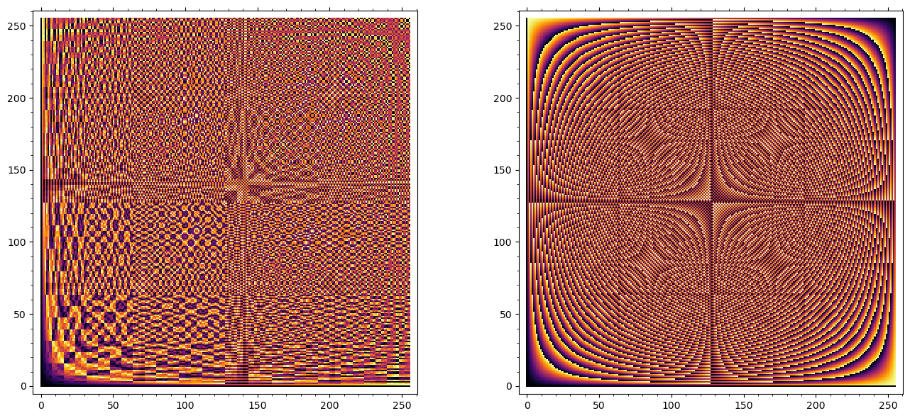
Experiment 1: Multiplication Table#
Heatmap
The full \(256 \times 256\) multiplication table of \(\mathrm{GF}(2^8)\) reveals the rich algebraic structure of the field. Unlike multiplication modulo \(n\) (which shows diagonal bands), the GF multiplication table has a pseudo-random, diffused appearance – precisely the property AES exploits for diffusion.
# Build GF(2^8) multiplication table using SageMath
mul_table = matrix(ZZ, 256, 256)
for i in range(256):
    ei = int_to_f256(i)
    for j in range(i, 256):
        ej = int_to_f256(j)
        p = f256_to_int(ei * ej)
        mul_table[i, j] = p
        mul_table[j, i] = p

# Compare: ordinary multiplication mod 256
ord_table = matrix(ZZ, 256, 256)
for i in range(256):
    for j in range(256):
        ord_table[i, j] = (i * j) % 256

p1 = matrix_plot(mul_table, cmap='inferno', origin='lower')
p2 = matrix_plot(ord_table, cmap='inferno', origin='lower')
graphics_array([p1, p2]).show(figsize=[14, 6])

print('Left: GF(2^8) multiplication -- pseudo-random, excellent diffusion.')
print('Right: ordinary mod-256 multiplication -- structured diagonal bands, poor diffusion.')
/opt/homebrew/Caskroom/miniconda/base/envs/sage/lib/python3.11/site-packages/sage/misc/decorators.py:507: DeprecationWarning: the option 'origin' is replaced by 'flip_y'
See https://github.com/sagemath/sage/issues/27891 for details.
  return func(*args, **options)
/opt/homebrew/Caskroom/miniconda/base/envs/sage/lib/python3.11/site-packages/sage/misc/decorators.py:507: DeprecationWarning: the option 'origin' is replaced by 'flip_y'
See https://github.com/sagemath/sage/issues/27891 for details.
  return func(*args, **options)
Left: GF(2^8) multiplication -- pseudo-random, excellent diffusion.
Right: ordinary mod-256 multiplication -- structured diagonal bands, poor diffusion.
Experiment 2: Verifying the Field Axioms#
A finite field must satisfy associativity, commutativity, distributivity, existence of identity elements, and existence of inverses. SageMath already guarantees these algebraically, but we verify them computationally as an exercise.
# Verify field axioms on random samples
set_random_seed(42)
N_TESTS = 50000

# Generate random elements using SageMath
aa_int = [randint(0, 255) for _ in range(N_TESTS)]
bb_int = [randint(0, 255) for _ in range(N_TESTS)]
cc_int = [randint(0, 255) for _ in range(N_TESTS)]

aa = [int_to_f256(v) for v in aa_int]
bb = [int_to_f256(v) for v in bb_int]
cc = [int_to_f256(v) for v in cc_int]

# 1. Commutativity of addition
assert all(aa[i] + bb[i] == bb[i] + aa[i] for i in range(N_TESTS))
print("[PASS] Commutativity of addition    (a + b == b + a)")

# 2. Commutativity of multiplication
assert all(aa[i] * bb[i] == bb[i] * aa[i] for i in range(N_TESTS))
print("[PASS] Commutativity of multiplication  (a * b == b * a)")

# 3. Associativity of addition
assert all((aa[i] + bb[i]) + cc[i] == aa[i] + (bb[i] + cc[i]) for i in range(N_TESTS))
print("[PASS] Associativity of addition    ((a+b)+c == a+(b+c))")

# 4. Associativity of multiplication
assert all((aa[i] * bb[i]) * cc[i] == aa[i] * (bb[i] * cc[i]) for i in range(N_TESTS))
print("[PASS] Associativity of multiplication  ((a*b)*c == a*(b*c))")

# 5. Distributivity
assert all(aa[i] * (bb[i] + cc[i]) == aa[i]*bb[i] + aa[i]*cc[i] for i in range(N_TESTS))
print("[PASS] Distributivity               (a*(b+c) == a*b + a*c)")

# 6. Additive identity
assert all(aa[i] + F256(0) == aa[i] for i in range(N_TESTS))
print("[PASS] Additive identity            (a + 0 == a)")

# 7. Multiplicative identity
assert all(aa[i] * F256(1) == aa[i] for i in range(N_TESTS))
print("[PASS] Multiplicative identity      (a * 1 == a)")

# 8. Additive inverse (in GF(2^n), every element is its own additive inverse)
assert all(aa[i] + aa[i] == F256(0) for i in range(N_TESTS))
print("[PASS] Additive inverse             (a + a == 0)")

# 9. Multiplicative inverse (exhaustive for all 255 nonzero elements)
all_pass = all(el * el^(-1) == F256(1) for el in F256 if el != F256(0))
assert all_pass
print("[PASS] Multiplicative inverse       (a * a^{-1} == 1 for all a != 0)")

print("\nAll field axioms verified on {:,} random samples (and exhaustive inverses).".format(N_TESTS))
[PASS] Commutativity of addition    (a + b == b + a)
[PASS] Commutativity of multiplication  (a * b == b * a)
[PASS] Associativity of addition    ((a+b)+c == a+(b+c))
[PASS] Associativity of multiplication  ((a*b)*c == a*(b*c))
[PASS] Distributivity               (a*(b+c) == a*b + a*c)
[PASS] Additive identity            (a + 0 == a)
[PASS] Multiplicative identity      (a * 1 == a)
[PASS] Additive inverse             (a + a == 0)
[PASS] Multiplicative inverse       (a * a^{-1} == 1 for all a != 0)

All field axioms verified on 50,000 random samples (and exhaustive inverses).
Experiment 3: Primitive Elements and Discrete Logarithms#
The multiplicative group \(\mathrm{GF}(2^8)^*\) is cyclic of order 255. SageMath can find generators (primitive elements) and compute discrete logarithms directly – no need for precomputed log/exp tables.
# Find the primitive element (generator) using SageMath
gen = F256.multiplicative_generator()
print("Multiplicative generator of GF(2^8)*:", gen)
print("As hex: 0x{}".format(g(gen)))
print()

# Verify: generator produces all 255 nonzero elements
generated = set()
val = F256(1)
for k in range(255):
    generated.add(val)
    val *= gen
print("Generator produces {} distinct nonzero elements.".format(len(generated)))

# Display first 32 entries of the exp table
print("\nExponentiation table (gen^k for k = 0..31):")
print("-" * 70)
for row_start in range(0, 32, 8):
    entries = []
    for k in range(row_start, row_start + 8):
        val = gen^k
        int_val = f256_to_int(val)
        entries.append("g^{:<2d}={:3d} (0x{})".format(k, int_val, g(val)))
    print("  " + "  ".join(entries))
Multiplicative generator of GF(2^8)*: a^4 + a + 1
As hex: 0x13

Generator produces 255 distinct nonzero elements.

Exponentiation table (gen^k for k = 0..31):
----------------------------------------------------------------------
  g^0 =  1 (0x01)  g^1 = 19 (0x13)  g^2 = 30 (0x1E)  g^3 =217 (0xD9)  g^4 = 79 (0x4F)  g^5 = 77 (0x4D)  g^6 =107 (0x6B)  g^7 = 87 (0x57)
  g^8 =254 (0xFE)  g^9 = 96 (0x60)  g^10=250 (0xFA)  g^11= 44 (0x2C)  g^12=130 (0x82)  g^13=101 (0x65)  g^14=165 (0xA5)  g^15= 74 (0x4A)
  g^16= 18 (0x12)  g^17= 13 (0x0D)  g^18=199 (0xC7)  g^19=150 (0x96)  g^20=  2 (0x02)  g^21= 38 (0x26)  g^22= 60 (0x3C)  g^23=169 (0xA9)
  g^24=158 (0x9E)  g^25=154 (0x9A)  g^26=214 (0xD6)  g^27=174 (0xAE)  g^28=231 (0xE7)  g^29=192 (0xC0)  g^30=239 (0xEF)  g^31= 88 (0x58)
# Discrete log visualization
gen = F256.multiplicative_generator()

# Build log and exp lists for plotting
log_vals = [0] * 256
exp_vals = [0] * 255
for k in range(255):
    val = gen^k
    int_val = f256_to_int(val)
    exp_vals[k] = int_val
    log_vals[int_val] = k

# Plot 1: Discrete log (a -> log_g(a))
p1 = scatter_plot([(a, log_vals[a]) for a in range(1, 256)],
                  markersize=3, facecolor='steelblue', alpha=0.8,
                  axes_labels=['Element a (integer repr.)', r'$\log_g(a)$'])

# Plot 2: Exponential (k -> g^k)
p2 = scatter_plot([(k, exp_vals[k]) for k in range(255)],
                  markersize=3, facecolor='purple', alpha=0.8,
                  axes_labels=['Exponent k', r'$g^k$'])

graphics_array([p1, p2]).show(figsize=[14, 5])

print("The discrete logarithm appears as a pseudo-random permutation of {0,...,254}.")
print("This 'randomness' is what makes discrete-log-based cryptography hard.")
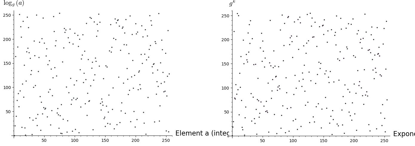
The discrete logarithm appears as a pseudo-random permutation of {0,...,254}.
This 'randomness' is what makes discrete-log-based cryptography hard.
Experiment 4: Computing Discrete Logs with SageMath#
SageMath provides a built-in log() method on finite field elements. This replaces the need for precomputed log/exp lookup tables entirely.
# SageMath's built-in discrete log
gen = F256.multiplicative_generator()
print("Discrete logarithms (base = generator 0x{}):".format(g(gen)))
print("-" * 50)
for hex_val in ['01', '02', '03', '09', '0B', '0D', '0E', '53', '57', 'FF']:
    el = h(hex_val)
    if el != F256(0):
        k = el.log(gen)
        print("  log(0x{}) = {:>3d}    verify: gen^{} = 0x{}".format(
            hex_val, k, k, g(gen^k)))

# Verify multiplication via logs
print("\nMultiplication via discrete logs:")
a_el, b_el = h('57'), h('83')
log_a = a_el.log(gen)
log_b = b_el.log(gen)
log_sum = (log_a + log_b) % 255
print("  log(0x57) = {}, log(0x83) = {}".format(log_a, log_b))
print("  log_sum mod 255 = {}".format(log_sum))
print("  gen^{} = 0x{}".format(log_sum, g(gen^log_sum)))
print("  Direct: 0x57 * 0x83 = 0x{}".format(g(a_el * b_el)))
Discrete logarithms (base = generator 0x13):
--------------------------------------------------
  log(0x01) =   0    verify: gen^0 = 0x01
  log(0x02) =  20    verify: gen^20 = 0x02
  log(0x03) = 164    verify: gen^164 = 0x03
  log(0x09) = 251    verify: gen^251 = 0x09
  log(0x0B) = 226    verify: gen^226 = 0x0B
  log(0x0D) =  17    verify: gen^17 = 0x0D
  log(0x0E) = 107    verify: gen^107 = 0x0E
  log(0x53) = 222    verify: gen^222 = 0x53
  log(0x57) =   7    verify: gen^7 = 0x57
  log(0xFF) = 128    verify: gen^128 = 0xFF

Multiplication via discrete logs:
  log(0x57) = 7, log(0x83) = 115
  log_sum mod 255 = 122
  gen^122 = 0xC1
  Direct: 0x57 * 0x83 = 0xC1
Experiment 5: Structure of the Multiplicative Group#
The multiplicative group \(\mathrm{GF}(2^8)^*\) is cyclic of order 255 = 3 x 5 x 17. Not every nonzero element is a generator. The order of an element \(a\) (the smallest \(k > 0\) with \(a^k = 1\)) must divide 255. SageMath can compute element orders directly via the multiplicative_order() method.
# SageMath provides built-in numerical tools
# SageMath provides built-in plotting

# Compute order of every nonzero element using SageMath's built-in method
orders = {}
for el in F256:
    if el != F256(0):
        orders[f256_to_int(el)] = el.multiplicative_order()

# Divisors of 255
print("255 =", factor(255))
divisors_255 = sorted(divisors(255))
print("Divisors of 255:", divisors_255)
print("Number of divisors:", len(divisors_255))

# Count elements of each order
print("\n{:>6s}  {:>6s}  {:>10s}".format('Order', 'Count', 'phi(order)'))
print("-" * 28)
for d in divisors_255:
    count = sum(1 for v in orders.values() if v == d)
    phi_d = euler_phi(d)
    print("  {:>4d}  {:>6d}  {:>10d}".format(d, count, phi_d))

generators_list = sorted([k for k, v in orders.items() if v == 255])
print("\nNumber of generators (primitive elements): {}".format(len(generators_list)))
print("Euler totient phi(255) = phi(3)*phi(5)*phi(17) = 2*4*16 = {}".format(euler_phi(255)))
print("First 10 generators: {}".format(['0x{:02X}'.format(gv) for gv in generators_list[:10]]))
255 = 3 * 5 * 17
Divisors of 255: [1, 3, 5, 15, 17, 51, 85, 255]
Number of divisors: 8

 Order   Count  phi(order)
----------------------------
     1       1           1
     3       2           2
     5       4           4
    15       8           8
    17      16          16
    51      32          32
    85      64          64
   255     128         128

Number of generators (primitive elements): 128
Euler totient phi(255) = phi(3)*phi(5)*phi(17) = 2*4*16 = 128
First 10 generators: ['0x03', '0x05', '0x06', '0x09', '0x0B', '0x0E', '0x11', '0x12', '0x13', '0x14']
# Plot order distribution using SageMath
order_counts = [(d, sum(1 for v in orders.values() if v == d)) for d in divisors_255]
bar_data = [c for _, c in order_counts]
labels = [str(d) for d in divisors_255]

P = bar_chart(bar_data, color='steelblue', width=0.8)
show(P, figsize=(10, 5),
     title='Distribution of element orders in GF(2^8)*',
     axes_labels=['Divisor index', 'Number of elements'])

# Print the divisor labels
for i, (d, c) in enumerate(order_counts):
    if c > 0:
        print(f'  Order {d}: {c} elements')
  Order 1: 1 elements
  Order 3: 2 elements
  Order 5: 4 elements
  Order 15: 8 elements
  Order 17: 16 elements
  Order 51: 32 elements
  Order 85: 64 elements
  Order 255: 128 elements
Experiment 6: The AES Inverse Table and S-Box Connection#
The AES S-box is constructed from two components:
The multiplicative inverse in \(\mathrm{GF}(2^8)\) (with \(0 \mapsto 0\)).
An affine transformation over \(\mathrm{GF}(2)\).
Let us visualize the inverse map. SageMath computes inverses with el^(-1) – no need for the manual extended GCD we built in the Python version.
# Build inverse table using SageMath's built-in inverse
inv_tbl = [0] * 256
for i in range(1, 256):
    el = int_to_f256(i)
    inv_el = el^(-1)
    inv_tbl[i] = f256_to_int(inv_el)

# Plot 1: Inverse map a -> a^{-1}
p1 = scatter_plot([(a, inv_tbl[a]) for a in range(256)],
                  markersize=4, facecolor='steelblue', alpha=0.8,
                  axes_labels=['a', r'$a^{-1}$'])

# Plot 2: Inverse as a 16x16 grid (byte value heatmap)
inv_grid = matrix(ZZ, 16, 16, [inv_tbl[16*r + c] for r in range(16) for c in range(16)])
p2 = matrix_plot(inv_grid, cmap='viridis')

graphics_array([p1, p2]).show(figsize=[14, 5])

# Verify involutory property: (a^{-1})^{-1} = a
assert all(int_to_f256(inv_tbl[inv_tbl[i]]) == int_to_f256(i)
           for i in range(1, 256))
print("Verified: (a^{-1})^{-1} = a for all nonzero elements.")

# Fixed points: a = a^{-1} means a^2 = 1
fixed = [i for i in range(256) if inv_tbl[i] == i]
print("Fixed points of the inverse map (a^2 = 1): {}".format(
    ['0x{:02X}'.format(a) for a in fixed]))
print("These are the square roots of unity in GF(2^8).")
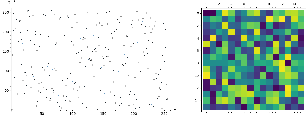
Verified: (a^{-1})^{-1} = a for all nonzero elements.
Fixed points of the inverse map (a^2 = 1): ['0x00', '0x01']
These are the square roots of unity in GF(2^8).
Experiment 7: Arithmetic in Small Extension Fields#
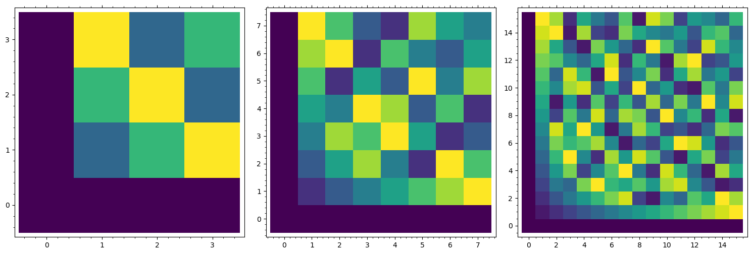
Before tackling \(\mathrm{GF}(2^8)\) in full, it is instructive to examine the smaller fields \(\mathrm{GF}(2^2)\), \(\mathrm{GF}(2^3)\), and \(\mathrm{GF}(2^4)\). These are small enough to display complete multiplication tables. SageMath constructs each with a single GF() call.
Note on the element 0
0 is not a unit in GF(2^8), so it is excluded from the group of units. The convention inv(0) = 0 used in AES is a special case for implementation convenience.
# Small fields using SageMath's built-in GF()
Rtemp.<xtemp> = PolynomialRing(GF(2))

small_fields = [
    ('GF(2^2)', GF(2^2, 'u'), 4),
    ('GF(2^3)', GF(2^3, 'v'), 8),
    ('GF(2^4)', GF(2^4, 'w'), 16),
]

plots = []
for idx, (name, field, size) in enumerate(small_fields):
    elements = list(field)
    # Convert field elements to integer representation
    def to_int_local(el):
        coeffs = Rtemp(el).list()
        return sum(int(c) * 2^i for i, c in enumerate(coeffs))

    el_by_int = {to_int_local(el): el for el in elements}
    mul_tbl = matrix(ZZ, size, size)
    for i in range(size):
        for j in range(size):
            mul_tbl[i, j] = to_int_local(el_by_int[i] * el_by_int[j])

    plots.append(matrix_plot(mul_tbl, cmap='viridis', origin='lower'))

graphics_array(plots).show(figsize=[15, 5])

# Print the full GF(2^2) multiplication table
print("\nComplete multiplication table for GF(2^2) = GF(2)[x]/(x^2+x+1):")
print("Elements: 0, 1, u, u+1  (as integers: 0, 1, 2, 3)")
F4s = GF(2^2, 'u')
els4 = list(F4s)
header = "{:>6s}".format("*")
for b in els4:
    header += "{:>6s}".format(str(b))
print(header)
print("-" * len(header))
for ai in els4:
    row = "{:>6s}".format(str(ai))
    for bi in els4:
        row += "{:>6s}".format(str(ai * bi))
    print(row)
/opt/homebrew/Caskroom/miniconda/base/envs/sage/lib/python3.11/site-packages/sage/misc/decorators.py:507: DeprecationWarning: the option 'origin' is replaced by 'flip_y'
See https://github.com/sagemath/sage/issues/27891 for details.
  return func(*args, **options)
Complete multiplication table for GF(2^2) = GF(2)[x]/(x^2+x+1):
Elements: 0, 1, u, u+1  (as integers: 0, 1, 2, 3)
     *     0     u u + 1     1
------------------------------
     0     0     0     0     0
     u     0 u + 1     1     u
 u + 1     0     1     u u + 1
     1     0     u u + 1     1
Experiment 8: Irreducible Polynomials of Degree 8 over GF(2)#
There are exactly 30 irreducible polynomials of degree 8 over \(\mathrm{GF}(2)\). Any of them could be used to construct \(\mathrm{GF}(2^8)\), producing isomorphic fields. The AES designers chose \(m(x) = x^8 + x^4 + x^3 + x + 1\) (the lexicographically first one with minimal nonzero terms after \(x^8\) and \(1\)).
In the Python version, we wrote a custom irreducibility test from scratch (~30 lines). SageMath provides is_irreducible() as a built-in method.
# Find all irreducible degree-8 polynomials over GF(2) using SageMath
R.<x> = PolynomialRing(GF(2))

irred_deg8 = []
for lower in range(256):
    # Build monic degree-8 polynomial
    coeffs = [(lower >> i) & 1 for i in range(8)]
    poly = x^8 + sum(GF(2)(coeffs[i]) * x^i for i in range(8))
    if poly.is_irreducible():
        irred_deg8.append(poly)

aes_modulus = x^8 + x^4 + x^3 + x + 1

print("Number of irreducible degree-8 polynomials over GF(2): {}".format(len(irred_deg8)))
print("\nAll {} polynomials:".format(len(irred_deg8)))
print("=" * 65)
for i, p in enumerate(irred_deg8):
    marker = "  <-- AES" if p == aes_modulus else ""
    # Convert to hex representation
    coeffs_list = p.list()
    hex_val = sum(int(coeffs_list[j]) * 2^j for j in range(len(coeffs_list)))
    print("  {:2d}. 0x{:03X}  =  {}{}".format(i+1, hex_val, p, marker))

# Verify count with the Necklace formula
print("\nFormula check: (2^8 - 2^4) / 8 = {}".format((256 - 16) // 8))
Number of irreducible degree-8 polynomials over GF(2): 30

All 30 polynomials:
=================================================================
   1. 0x11B  =  x^8 + x^4 + x^3 + x + 1  <-- AES
   2. 0x11D  =  x^8 + x^4 + x^3 + x^2 + 1
   3. 0x12B  =  x^8 + x^5 + x^3 + x + 1
   4. 0x12D  =  x^8 + x^5 + x^3 + x^2 + 1
   5. 0x139  =  x^8 + x^5 + x^4 + x^3 + 1
   6. 0x13F  =  x^8 + x^5 + x^4 + x^3 + x^2 + x + 1
   7. 0x14D  =  x^8 + x^6 + x^3 + x^2 + 1
   8. 0x15F  =  x^8 + x^6 + x^4 + x^3 + x^2 + x + 1
   9. 0x163  =  x^8 + x^6 + x^5 + x + 1
  10. 0x165  =  x^8 + x^6 + x^5 + x^2 + 1
  11. 0x169  =  x^8 + x^6 + x^5 + x^3 + 1
  12. 0x171  =  x^8 + x^6 + x^5 + x^4 + 1
  13. 0x177  =  x^8 + x^6 + x^5 + x^4 + x^2 + x + 1
  14. 0x17B  =  x^8 + x^6 + x^5 + x^4 + x^3 + x + 1
  15. 0x187  =  x^8 + x^7 + x^2 + x + 1
  16. 0x18B  =  x^8 + x^7 + x^3 + x + 1
  17. 0x18D  =  x^8 + x^7 + x^3 + x^2 + 1
  18. 0x19F  =  x^8 + x^7 + x^4 + x^3 + x^2 + x + 1
  19. 0x1A3  =  x^8 + x^7 + x^5 + x + 1
  20. 0x1A9  =  x^8 + x^7 + x^5 + x^3 + 1
  21. 0x1B1  =  x^8 + x^7 + x^5 + x^4 + 1
  22. 0x1BD  =  x^8 + x^7 + x^5 + x^4 + x^3 + x^2 + 1
  23. 0x1C3  =  x^8 + x^7 + x^6 + x + 1
  24. 0x1CF  =  x^8 + x^7 + x^6 + x^3 + x^2 + x + 1
  25. 0x1D7  =  x^8 + x^7 + x^6 + x^4 + x^2 + x + 1
  26. 0x1DD  =  x^8 + x^7 + x^6 + x^4 + x^3 + x^2 + 1
  27. 0x1E7  =  x^8 + x^7 + x^6 + x^5 + x^2 + x + 1
  28. 0x1F3  =  x^8 + x^7 + x^6 + x^5 + x^4 + x + 1
  29. 0x1F5  =  x^8 + x^7 + x^6 + x^5 + x^4 + x^2 + 1
  30. 0x1F9  =  x^8 + x^7 + x^6 + x^5 + x^4 + x^3 + 1

Formula check: (2^8 - 2^4) / 8 = 30
Experiment 9: The Extended Euclidean Algorithm in SageMath#
The extended Euclidean algorithm for polynomials over \(\mathrm{GF}(2)\) is the heart of the inverse computation. SageMath’s xgcd() function computes this in one call. Let us trace through examples and verify.
# SageMath's xgcd does the extended GCD in one line
R.<x> = PolynomialRing(GF(2))
m = x^8 + x^4 + x^3 + x + 1

# Example 1: inverse of 0x53 in the polynomial ring
a_poly = R(list(map(int, reversed(bin(0x53)[2:].zfill(8)))))
print("Example 1: Finding inverse of a(x) = {} (0x53)".format(a_poly))
print("Modulus m(x) =", m)
print()

# Use SageMath's xgcd
d, s, t = xgcd(a_poly, m)
print("xgcd(a, m) returns:")
print("  gcd = {}".format(d))
print("  s(x) = {}".format(s))
print("  t(x) = {}".format(t))
print("  Verify: s*a + t*m = {}".format(s * a_poly + t * m))
print()

# The inverse is s(x) mod m(x)
s_reduced = s % m
print("Inverse s(x) mod m(x) = {}".format(s_reduced))

# Convert to F256 and verify
a_field = h('53')
inv_field = a_field^(-1)
print("Direct computation: (0x53)^(-1) = 0x{} = {}".format(g(inv_field), inv_field))
print("Verify: 0x53 * 0x{} = 0x{}".format(g(inv_field), g(a_field * inv_field)))

print()
print("=" * 60)
print()

# Example 2: inverse of 0x03 (AES generator)
a_poly2 = x + 1  # 0x03 = x + 1
print("Example 2: Finding inverse of a(x) = {} (0x03, the AES generator)".format(a_poly2))
d2, s2, t2 = xgcd(a_poly2, m)
print("  gcd = {}".format(d2))
print("  s(x) = {}".format(s2))
print("  Inverse: {}".format(s2 % m))

inv_03 = h('03')^(-1)
print("  Direct: (0x03)^(-1) = 0x{} = {}".format(g(inv_03), inv_03))
Example 1: Finding inverse of a(x) = x^6 + x^4 + x + 1 (0x53)
Modulus m(x) = x^8 + x^4 + x^3 + x + 1

xgcd(a, m) returns:
  gcd = 1
  s(x) = x^7 + x^6 + x^3 + x
  t(x) = x^5 + x^4 + x^3 + x^2 + 1
  Verify: s*a + t*m = 1

Inverse s(x) mod m(x) = x^7 + x^6 + x^3 + x
Direct computation: (0x53)^(-1) = 0xCA = a^7 + a^6 + a^3 + a
Verify: 0x53 * 0xCA = 0x01

============================================================

Example 2: Finding inverse of a(x) = x + 1 (0x03, the AES generator)
  gcd = 1
  s(x) = x^7 + x^6 + x^5 + x^4 + x^2 + x
  Inverse: x^7 + x^6 + x^5 + x^4 + x^2 + x
  Direct: (0x03)^(-1) = 0xF6 = a^7 + a^6 + a^5 + a^4 + a^2 + a
Experiment 10: Output Distribution of GF(2^8) Multiplication#
A key property of field multiplication (vs. ring multiplication modulo \(2^8\)) is that for any fixed nonzero \(a\), the map \(b \mapsto a \cdot b\) is a permutation of \(\mathrm{GF}(2^8)\). This is precisely what makes it useful for diffusion in AES MixColumns.
# Values used in AES MixColumns
test_values = ['02', '03', '09', '0B', '0D', '0E']

plots = []
for idx, a_hex in enumerate(test_values):
    a_el = h(a_hex)

    # Compute all products a * b for b in GF(2^8)
    products = [f256_to_int(a_el * int_to_f256(b)) for b in range(256)]

    # Check permutation property
    is_perm = len(set(products)) == 256
    perm_str = 'Perm' if is_perm else 'NOT perm'

    from collections import Counter
    hist_data = Counter(products)
    bar_data = [hist_data.get(v, 0) for v in range(256)]

    p = bar_chart(bar_data, color='steelblue', width=1)
    plots.append(p)
    print(f'a = 0x{a_hex} ({a_el}): {perm_str}, {len(set(products))} distinct outputs')

# Show first 3 plots
graphics_array(plots[:3]).show(figsize=[15, 4])
graphics_array(plots[3:]).show(figsize=[15, 4])

# Contrast with ordinary mod-256 multiplication
print("\nContrast: ordinary multiplication mod 256")
print("-" * 50)
for a_int in [2, 3, 4, 6]:
    products_ord = set((a_int * b) % 256 for b in range(256))
    print("  a={}: {} distinct outputs out of 256  ({})".format(
        a_int, len(products_ord),
        'permutation' if len(products_ord) == 256 else 'NOT permutation'))
a = 0x02 (a): Perm, 256 distinct outputs
a = 0x03 (a + 1): Perm, 256 distinct outputs
a = 0x09 (a^3 + 1): Perm, 256 distinct outputs
a = 0x0B (a^3 + a + 1): Perm, 256 distinct outputs
a = 0x0D (a^3 + a^2 + 1): Perm, 256 distinct outputs
a = 0x0E (a^3 + a^2 + a): Perm, 256 distinct outputs
Contrast: ordinary multiplication mod 256
--------------------------------------------------
  a=2: 128 distinct outputs out of 256  (NOT permutation)
  a=3: 256 distinct outputs out of 256  (permutation)
  a=4: 64 distinct outputs out of 256  (NOT permutation)
  a=6: 128 distinct outputs out of 256  (NOT permutation)
Experiment 11: SageMath vs Python – Comparing Approaches#
This experiment highlights the dramatic simplification that SageMath provides. The table below compares what each operation requires in the Python version vs. SageMath.
# Side-by-side comparison: operations that took many lines in Python
# are one-liners in SageMath

print("Operation Comparison: Python (ch22) vs SageMath")
print("=" * 65)
print()

comparisons = [
    ("Construct GF(2^8)",
     "class GF256: ... (~200 lines)",
     "GF(2^8, modulus=...)"),
    ("Multiply two elements",
     "GF256.multiply(a, b)  # shift-and-XOR loop",
     "a * b"),
    ("Compute inverse",
     "GF256.inverse(a)  # extended GCD ~40 lines",
     "a^(-1)"),
    ("Element order",
     "element_order(a)  # manual loop",
     "a.multiplicative_order()"),
    ("Find generators",
     "[a for a in range(1,256) if order(a)==255]",
     "F.multiplicative_generator()"),
    ("Irreducibility test",
     "is_irreducible_gf2(poly)  # ~30 lines",
     "poly.is_irreducible()"),
    ("Discrete logarithm",
     "log_table[a]  # precomputed array",
     "a.log(gen)"),
    ("Polynomial GCD",
     "GF256._poly_divmod()  # custom impl",
     "gcd(a, b)  or  xgcd(a, b)"),
]

for operation, python_way, sage_way in comparisons:
    print("{}".format(operation))
    print("  Python:   {}".format(python_way))
    print("  SageMath: {}".format(sage_way))
    print()

print("SageMath replaces ~300 lines of manual finite field code")
print("with built-in, optimized, and mathematically verified operations.")
Operation Comparison: Python (ch22) vs SageMath
=================================================================

Construct GF(2^8)
  Python:   class GF256: ... (~200 lines)
  SageMath: GF(2^8, modulus=...)

Multiply two elements
  Python:   GF256.multiply(a, b)  # shift-and-XOR loop
  SageMath: a * b

Compute inverse
  Python:   GF256.inverse(a)  # extended GCD ~40 lines
  SageMath: a^(-1)

Element order
  Python:   element_order(a)  # manual loop
  SageMath: a.multiplicative_order()

Find generators
  Python:   [a for a in range(1,256) if order(a)==255]
  SageMath: F.multiplicative_generator()

Irreducibility test
  Python:   is_irreducible_gf2(poly)  # ~30 lines
  SageMath: poly.is_irreducible()

Discrete logarithm
  Python:   log_table[a]  # precomputed array
  SageMath: a.log(gen)

Polynomial GCD
  Python:   GF256._poly_divmod()  # custom impl
  SageMath: gcd(a, b)  or  xgcd(a, b)

SageMath replaces ~300 lines of manual finite field code
with built-in, optimized, and mathematically verified operations.
Experiment 12: Powers of the Generator in the AES Field#
Let us list powers of the generator element a (corresponding to \(x\) in the quotient ring) and verify its order.
# Powers of the generator a in F256
# (a represents x in GF(2)[x]/(m(x)))
print("First 15 powers of a (the image of x in the quotient field):")
for k in range(15):
    print("  a^{:<3d} = {:30s} = 0x{}".format(k, str(a^k), g(a^k)))

print()
print("Multiplicative order of a:", a.multiplicative_order())
print("Is a a primitive element?", a.multiplicative_order() == 255)

# Also check 0x03 = a + 1
gen_03 = a + F256(1)
print()
print("Element a+1 (= 0x03):", gen_03, "= 0x" + g(gen_03))
print("Multiplicative order of a+1:", gen_03.multiplicative_order())
print("Is 0x03 a primitive element?", gen_03.multiplicative_order() == 255)
First 15 powers of a (the image of x in the quotient field):
  a^0   = 1                              = 0x01
  a^1   = a                              = 0x02
  a^2   = a^2                            = 0x04
  a^3   = a^3                            = 0x08
  a^4   = a^4                            = 0x10
  a^5   = a^5                            = 0x20
  a^6   = a^6                            = 0x40
  a^7   = a^7                            = 0x80
  a^8   = a^4 + a^3 + a + 1              = 0x1B
  a^9   = a^5 + a^4 + a^2 + a            = 0x36
  a^10  = a^6 + a^5 + a^3 + a^2          = 0x6C
  a^11  = a^7 + a^6 + a^4 + a^3          = 0xD8
  a^12  = a^7 + a^5 + a^3 + a + 1        = 0xAB
  a^13  = a^6 + a^3 + a^2 + 1            = 0x4D
  a^14  = a^7 + a^4 + a^3 + a            = 0x9A

Multiplicative order of a: 51
Is a a primitive element? False

Element a+1 (= 0x03): a + 1 = 0x03
Multiplicative order of a+1: 255
Is 0x03 a primitive element? True
22.5 Exercises#
Exercise 22.1: Hand Computation with SageMath Verification#
Compute \(\{\mathtt{0xAB}\} \cdot \{\mathtt{0xCD}\}\) in \(\mathrm{GF}(2^8)\) by hand. Write out both polynomials, perform the full polynomial multiplication over \(\mathrm{GF}(2)\), and reduce modulo \(m(x) = x^8 + x^4 + x^3 + x + 1\). Then verify with SageMath.
Hint
\(\mathtt{0xAB} = x^7 + x^5 + x^3 + x + 1\) and \(\mathtt{0xCD} = x^7 + x^6 + x^3 + x^2 + 1\). In SageMath, simply compute h('AB') * h('CD') and verify it equals 0x6B.
Exercise 22.2: Proving Irreducibility with SageMath#
Verify that \(m(x) = x^8 + x^4 + x^3 + x + 1\) is irreducible over \(\mathrm{GF}(2)\) using SageMath. Then find all irreducible polynomials of degree 8 that are also primitive (i.e., the quotient field’s generator \(x\) has maximal order 255).
Hint
Use poly.is_irreducible() and then for each irreducible polynomial, construct the field and check if the generator has order 255. Not all irreducible polynomials are primitive!
Exercise 22.3: Subfield Structure#
Show that \(\mathrm{GF}(2^8)\) contains exactly one copy of \(\mathrm{GF}(2^2)\) and one copy of \(\mathrm{GF}(2^4)\) as subfields. Find the elements of each subfield explicitly using SageMath.
Hint
The elements of \(\mathrm{GF}(2^d)\) inside \(\mathrm{GF}(2^8)\) are exactly the roots of \(x^{2^d} - x = x^{2^d} + x\). In SageMath: [el for el in F256 if el^(2^d) == el]. For \(d=2\), this gives the 4 elements of the embedded \(\mathrm{GF}(4)\).
Exercise 22.4: Fermat’s Little Theorem in GF(2^8)#
Show that for every nonzero \(a \in \mathrm{GF}(2^8)\), we have \(a^{255} = 1\), and therefore \(a^{-1} = a^{254}\). Verify computationally using SageMath.
Hint
Simply verify: all(el^255 == F256(1) for el in F256 if el != F256(0)) and all(el^254 == el^(-1) for el in F256 if el != F256(0)).
Exercise 22.5: The xtime Operation and MixColumns Constants#
The AES specification defines xtime as multiplication by \(x\) (i.e., by \(\mathtt{0x02}\)) in \(\mathrm{GF}(2^8)\). Verify using SageMath that multiplication by 0x03, 0x09, 0x0B, 0x0D, and 0x0E can be decomposed into chains of xtime and XOR. Show these decompositions.
Hint
In SageMath, h('02') is simply a (the generator). So xtime is multiplication by a. For example, multiplication by 0x03 = a + 1 is: a*b + b. Verify: all(h('03') * int_to_f256(b) == a * int_to_f256(b) + int_to_f256(b) for b in range(256)).
# Exercise workspace
# Try the exercises here!

# Exercise 22.1 verification:
print("Exercise 22.1:")
print("  0xAB * 0xCD =", g(h('AB') * h('CD')))

# Exercise 22.4 verification (Fermat's Little Theorem):
print("\nExercise 22.4 (Fermat's Little Theorem):")
print("  All a^255 == 1?", all(el^255 == F256(1) for el in F256 if el != F256(0)))
print("  All a^254 == a^(-1)?", all(el^254 == el^(-1) for el in F256 if el != F256(0)))
Exercise 22.1:
  0xAB * 0xCD = BB

Exercise 22.4 (Fermat's Little Theorem):
  All a^255 == 1? True
  All a^254 == a^(-1)? True
22.6 Summary and Key Takeaways#
In this chapter, we have explored \(\mathrm{GF}(2^8)\) arithmetic using SageMath’s built-in finite field capabilities:
Field construction.
GF(2^8, modulus=x^8+x^4+x^3+x+1)creates the AES field in one line, replacing the entireGF256class from the Python version.Effortless arithmetic. Addition, multiplication, inversion, and exponentiation are all native operations:
a + b,a * b,a^(-1),a^n. SageMath handles polynomial multiplication and modular reduction automatically.Built-in algebraic tools.
is_irreducible(),multiplicative_order(),multiplicative_generator(),xgcd(), andlog()replace hundreds of lines of custom code.Diffusion property. Multiplication by any nonzero field element is a permutation of all 256 values – a property that \(\mathbb{Z}_{256}\) (integers mod 256) does not share. This is why AES uses GF multiplication in MixColumns.
Cyclic multiplicative group. \(\mathrm{GF}(2^8)^*\) is cyclic of order 255, and SageMath can find generators and compute discrete logarithms directly.
Tip
The choice of \(\mathrm{GF}(2^8)\) in AES is not arbitrary – it is the unique algebraic structure that simultaneously provides byte-level compatibility, efficient hardware/software implementation, and the nonlinear inverse map that is the foundation of the S-box’s cryptographic strength.
SageMath Summary
This chapter demonstrates SageMath’s key advantage for algebraic cryptanalysis: the ability to work at a mathematical level of abstraction without reimplementing standard algebraic constructions. For \(\mathrm{GF}(2^8)\), SageMath replaces ~300 lines of manual Python with built-in, optimized operations – freeing the cryptanalyst to focus on the mathematics rather than the implementation.
What comes next: In Chapter 23, we will use the \(\mathrm{GF}(2^8)\) arithmetic developed here to construct the AES S-box and analyze its cryptographic properties.
22.7 References#
Daemen, J. and Rijmen, V. (2002). The Design of Rijndael: AES – The Advanced Encryption Standard. Springer-Verlag. The definitive reference by the AES designers. Chapter 2 covers the algebraic preliminaries including \(\mathrm{GF}(2^8)\) arithmetic in detail.
NIST (2001). FIPS 197: Advanced Encryption Standard (AES). National Institute of Standards and Technology. The official AES specification. Section 4 defines the finite field arithmetic used throughout the cipher.
Lidl, R. and Niederreiter, H. (1997). Finite Fields, 2nd ed. Cambridge University Press. Comprehensive mathematical treatment of finite fields, including construction, structure, and applications.
Mullen, G. L. and Panario, D. (2013). Handbook of Finite Fields. CRC Press. An encyclopedic reference covering all aspects of finite field theory and computation.
Galois, E. (1846). “Sur les conditions de resolubilite des equations par radicaux.” Journal de Mathematiques Pures et Appliquees, 11, 417–433. The posthumously published paper that founded the theory of finite fields.
SageMath Documentation. Finite Fields. https://doc.sagemath.org/html/en/reference/finite_rings/ Official SageMath documentation for finite field constructions and arithmetic.