Chapter 40: Lattice Problems — SVP, CVP, and LWE

Chapter 40: Lattice Problems — SVP, CVP, and LWE#

40.1 Introduction and Historical Context#

Lattice-based cryptography has emerged as the leading candidate for post-quantum public-key cryptography. Its foundations rest on the computational hardness of geometric problems in high-dimensional integer lattices.

Key milestones:

Year	Contribution	Significance
1982	Lenstra–Lenstra–Lovász (LLL) algorithm	Polynomial-time lattice basis reduction
1996	Ajtai’s worst-case/average-case reduction	Average-case hardness of lattice problems implies worst-case hardness
1997	Ajtai–Dwork cryptosystem	First lattice-based encryption scheme
2005	Regev’s Learning With Errors (LWE)	Versatile hard problem with quantum reduction to worst-case lattice problems
2010	Lyubashevsky–Peikert–Regev Ring-LWE	Efficient structured variant of LWE
2022	NIST selects CRYSTALS-Kyber/Dilithium	Lattice-based schemes become standards

Ajtai’s 1996 breakthrough showed that if any instance of certain lattice problems (like the Shortest Vector Problem) is hard in the worst case, then random instances of related problems are also hard on average. This is a much stronger security guarantee than, say, RSA, where we only assume that random products of primes are hard to factor.

Regev’s 2005 LWE problem provides a clean algebraic framework: given a system of “noisy” linear equations modulo \(q\), recover the secret. He proved (using a quantum reduction) that solving LWE is at least as hard as solving worst-case lattice problems like GapSVP.

Why lattices for post-quantum?

Unlike RSA and elliptic-curve schemes, no known quantum algorithm solves lattice problems (SVP, CVP, LWE) in polynomial time. Shor’s algorithm breaks factoring and discrete log, but lattice problems appear to resist both classical and quantum attacks.

40.2 Definitions#

40.2.1 Lattice#

Definition — Lattice

A lattice \(\mathcal{L}(B)\) generated by a basis \(B = [\mathbf{b}_1, \ldots, \mathbf{b}_n] \in \mathbb{R}^{m \times n}\) is the set of all integer linear combinations of the basis vectors:

\[ \mathcal{L}(B) = \left\{ B\mathbf{x} : \mathbf{x} \in \mathbb{Z}^n \right\} = \left\{ \sum_{i=1}^{n} x_i \mathbf{b}_i : x_i \in \mathbb{Z} \right\}\]

The integer \(n\) is the rank (or dimension) of the lattice; \(m \ge n\) is the ambient dimension.

A lattice is a discrete additive subgroup of \(\mathbb{R}^m\). Unlike a vector space, a lattice has “gaps” — there is a minimum nonzero distance between any two lattice points.

40.2.2 Shortest Vector Problem (SVP)#

Definition — SVP

Given a basis \(B\) of a lattice \(\mathcal{L}\), the Shortest Vector Problem asks to find a nonzero lattice vector \(\mathbf{v} \in \mathcal{L} \setminus \{\mathbf{0}\}\) such that

\[ \|\mathbf{v}\| = \lambda_1(\mathcal{L}) := \min_{\mathbf{w} \in \mathcal{L} \setminus \{0\}} \|\mathbf{w}\|\]

where \(\|\cdot\|\) denotes the Euclidean norm.

40.2.3 Closest Vector Problem (CVP)#

Definition — CVP

Given a basis \(B\) of a lattice \(\mathcal{L}\) and a target vector \(\mathbf{t} \in \mathbb{R}^m\), the Closest Vector Problem asks to find a lattice vector \(\mathbf{v} \in \mathcal{L}\) that minimizes \(\|\mathbf{v} - \mathbf{t}\|\).

CVP is at least as hard as SVP (in a complexity-theoretic sense). Both are NP-hard in their exact versions, and believed hard to approximate within polynomial factors.

40.2.4 Learning With Errors (LWE)#

Definition — LWE

Fix integers \(n\) (dimension), \(q\) (modulus), and an error distribution \(\chi\) (typically a discrete Gaussian with standard deviation \(\sigma\)). The Learning With Errors problem, for a secret \(\mathbf{s} \in \mathbb{Z}_q^n\), is:

Given polynomially many samples \((\mathbf{a}_i, b_i) \in \mathbb{Z}_q^n \times \mathbb{Z}_q\) where

\[ b_i = \langle \mathbf{a}_i, \mathbf{s} \rangle + e_i \pmod{q}, \quad e_i \leftarrow \chi\]

recover the secret \(\mathbf{s}\).

In matrix form: given \((A, \mathbf{b} = A\mathbf{s} + \mathbf{e} \pmod{q})\), find \(\mathbf{s}\).

Without the error \(\mathbf{e}\), this is simply solving a linear system mod \(q\) — trivial via Gaussian elimination. The noise is what makes LWE hard.

40.2.5 Ring-LWE and Module-LWE#

Definition — Ring-LWE

Ring-LWE restricts LWE to the polynomial ring \(R_q = \mathbb{Z}_q[x]/(x^n + 1)\). The secret, samples, and errors are all elements of \(R_q\), enabling \(O(n \log n)\) operations via NTT (Number Theoretic Transform). Module-LWE generalizes to vectors over \(R_q\), bridging Ring-LWE and standard LWE.

CRYSTALS-Kyber (now ML-KEM) is based on Module-LWE; CRYSTALS-Dilithium (ML-DSA) is based on Module-LWE and Module-SIS.

40.2.6 Ajtai’s Reduction (Conceptual)#

Theorem — Ajtai (1996)

If there exists a polynomial-time algorithm that solves the average-case Short Integer Solution (SIS) problem, then there exists a polynomial-time algorithm that solves worst-case approximate SVP (within polynomial factors) on any lattice.

This is remarkable: it means that to build a cryptosystem, we can sample a random instance and be confident that breaking it is as hard as solving the hardest lattice problems.

40.3 Lattice Class with Gram-Schmidt and LLL Reduction#

We implement a Lattice class that stores a basis and supports Gram-Schmidt orthogonalization and LLL basis reduction. All implementations use only NumPy.

import numpy as np
import math

class Lattice:
    """Integer lattice with basis reduction capabilities.

    Parameters
    ----------
    basis : array-like, shape (n, m)
        Row vectors forming the lattice basis. Each row is a basis vector.
    """

    def __init__(self, basis):
        self.basis = np.array(basis, dtype=float)
        self.n = self.basis.shape[0]   # rank (number of basis vectors)
        self.m = self.basis.shape[1]   # ambient dimension

    def gram_schmidt(self):
        """Compute the Gram-Schmidt orthogonalization of the basis.

        Returns
        -------
        Q : ndarray, shape (n, m)
            Orthogonalized basis vectors (not normalized).
        mu : ndarray, shape (n, n)
            GSO coefficients: basis[i] = Q[i] + sum_j<i mu[i,j]*Q[j].
        """
        n, m = self.n, self.m
        Q = np.zeros((n, m))
        mu = np.zeros((n, n))

        for i in range(n):
            Q[i] = self.basis[i].copy()
            for j in range(i):
                if np.dot(Q[j], Q[j]) < 1e-14:
                    mu[i, j] = 0.0
                else:
                    mu[i, j] = np.dot(self.basis[i], Q[j]) / np.dot(Q[j], Q[j])
                Q[i] -= mu[i, j] * Q[j]

        return Q, mu

    def hadamard_ratio(self):
        """Compute the Hadamard ratio — a measure of basis orthogonality.

        Returns 1.0 for a perfectly orthogonal basis, near 0 for a bad basis.
        """
        det = abs(np.linalg.det(self.basis[:self.n, :self.n])) if self.n == self.m else \
              abs(np.sqrt(np.linalg.det(self.basis @ self.basis.T)))
        norms_product = np.prod(np.linalg.norm(self.basis, axis=1))
        if norms_product < 1e-14:
            return 0.0
        return (det / norms_product) ** (1.0 / self.n)

    def shortest_vector_enum_2d(self):
        """Find the shortest nonzero vector by enumeration (only for 2D lattices)."""
        assert self.n == 2 and self.m == 2, "Only for 2D lattices"
        b1, b2 = self.basis[0], self.basis[1]
        best_norm = float('inf')
        best_vec = None
        R = 20  # search radius
        for i in range(-R, R + 1):
            for j in range(-R, R + 1):
                if i == 0 and j == 0:
                    continue
                v = i * b1 + j * b2
                norm_v = np.linalg.norm(v)
                if norm_v < best_norm:
                    best_norm = norm_v
                    best_vec = v.copy()
        return best_vec, best_norm

    def copy(self):
        return Lattice(self.basis.copy())

    def __repr__(self):
        return f"Lattice(rank={self.n}, ambient_dim={self.m}, hadamard_ratio={float(self.hadamard_ratio()):.4f})"

# Quick test
B = np.array([[1, 0], [0.5, np.sqrt(3)/2]])
L = Lattice(B)
Q, mu = L.gram_schmidt()
print(f"Lattice: {L}")
print(f"Basis:\n{L.basis}")
print(f"Gram-Schmidt Q:\n{Q}")
print(f"GSO coefficients mu:\n{mu}")
print(f"Hadamard ratio: {float(L.hadamard_ratio()):.4f}")

Lattice: Lattice(rank=2, ambient_dim=2, hadamard_ratio=0.9306)
Basis:
[[1.        0.       ]
 [0.5       0.8660254]]
Gram-Schmidt Q:
[[1.        0.       ]
 [0.        0.8660254]]
GSO coefficients mu:
[[0.  0. ]
 [0.5 0. ]]
Hadamard ratio: 0.9306

40.4 LLL Basis Reduction Algorithm#

The Lenstra-Lenstra-Lovász (LLL) algorithm (1982) is a polynomial-time lattice basis reduction algorithm. Given a basis \(B\), it produces a reduced basis \(B'\) whose vectors are “more orthogonal” and shorter. Specifically, an LLL-reduced basis with parameter \(\delta\) satisfies:

Size reduction: \(|\mu_{i,j}| \le 1/2\) for all \(j < i\).
Lovász condition: \(\delta \|\mathbf{b}^*_i\|^2 \le \|\mathbf{b}^*_{i+1} + \mu_{i+1,i}\mathbf{b}^*_i\|^2\) for all \(i\).

The first basis vector of an LLL-reduced basis satisfies:

\[ \|\mathbf{b}_1\| \le 2^{(n-1)/2} \cdot \lambda_1(\mathcal{L})\]

This is an exponential approximation factor, but the algorithm runs in polynomial time.

import numpy as np
import math

def lll_reduce(basis, delta=0.75):
    """LLL lattice basis reduction algorithm.

    Parameters
    ----------
    basis : array-like, shape (n, m)
        Row vectors forming the lattice basis.
    delta : float, optional
        Lovász condition parameter, 0.25 < delta <= 1.0. Default 0.75.

    Returns
    -------
    reduced_basis : ndarray
        LLL-reduced basis (row vectors).
    """
    B = np.array(basis, dtype=float)
    n = B.shape[0]

    def compute_gso(B):
        """Compute Gram-Schmidt orthogonalization."""
        n, m = B.shape
        Q = np.zeros_like(B)
        mu = np.zeros((n, n))
        for i in range(n):
            Q[i] = B[i].copy()
            for j in range(i):
                denom = np.dot(Q[j], Q[j])
                if denom < 1e-14:
                    mu[i, j] = 0.0
                else:
                    mu[i, j] = np.dot(B[i], Q[j]) / denom
                Q[i] -= mu[i, j] * Q[j]
        return Q, mu

    k = 1
    while k < n:
        Q, mu = compute_gso(B)

        # Size reduction
        for j in range(k - 1, -1, -1):
            if abs(mu[k, j]) > 0.5:
                B[k] -= round(mu[k, j]) * B[j]
                Q, mu = compute_gso(B)

        # Lovász condition
        lhs = delta * np.dot(Q[k-1], Q[k-1])
        rhs = np.dot(Q[k], Q[k]) + mu[k, k-1]**2 * np.dot(Q[k-1], Q[k-1])

        if lhs > rhs:
            # Swap b_k and b_{k-1}
            B[[k, k-1]] = B[[k-1, k]]
            k = max(k - 1, 1)
        else:
            k += 1

    return B

# Test on a 2D example
B_bad = np.array([[1, 1], [0, 107]], dtype=float)
B_reduced = lll_reduce(B_bad)

print("Original basis:")
print(B_bad)
print(f"Norms: {float(np.linalg.norm(B_bad[0])):.2f}, {float(np.linalg.norm(B_bad[1])):.2f}")
print(f"Hadamard ratio: {float(Lattice(B_bad).hadamard_ratio()):.4f}")
print()
print("LLL-reduced basis:")
print(B_reduced)
print(f"Norms: {float(np.linalg.norm(B_reduced[0])):.2f}, {float(np.linalg.norm(B_reduced[1])):.2f}")
print(f"Hadamard ratio: {float(Lattice(B_reduced).hadamard_ratio()):.4f}")

Original basis:
[[  1.   1.]
 [  0. 107.]]
Norms: 1.41, 107.00
Hadamard ratio: 0.8409

LLL-reduced basis:
[[  1.   1.]
 [-54.  53.]]
Norms: 1.41, 75.66
Hadamard ratio: 1.0000

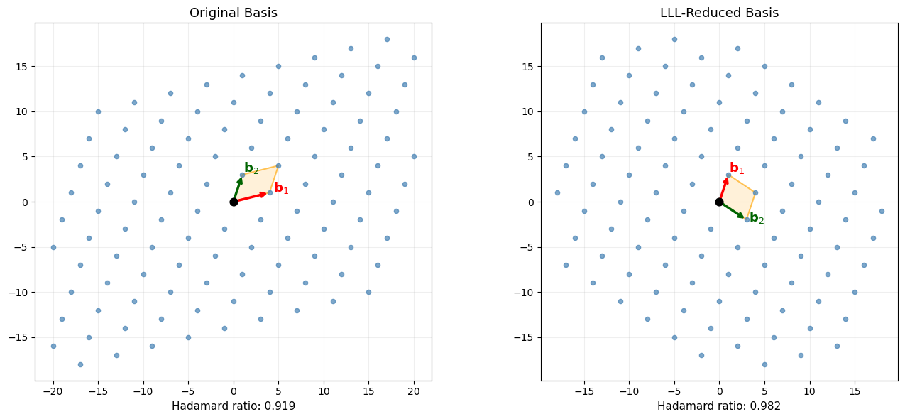
40.5 Visualizing 2D Lattices#

We visualize a 2D lattice, its fundamental domain, and the effect of LLL reduction on the basis vectors.

Show code cell source Hide code cell source

import numpy as np
import matplotlib.pyplot as plt
import math

def plot_lattice_2d(basis, ax, title="2D Lattice", R=6, show_fundamental=True):
    """Plot a 2D lattice with its basis vectors and lattice points."""
    b1, b2 = basis[0], basis[1]

    # Generate lattice points
    points = []
    for i in range(-R, R + 1):
        for j in range(-R, R + 1):
            pt = i * b1 + j * b2
            if abs(pt[0]) < R * max(np.linalg.norm(b1), np.linalg.norm(b2)) and \
               abs(pt[1]) < R * max(np.linalg.norm(b1), np.linalg.norm(b2)):
                points.append(pt)
    points = np.array(points)

    ax.scatter(points[:, 0], points[:, 1], c='steelblue', s=20, zorder=3, alpha=0.7)

    # Draw basis vectors
    origin = np.array([0, 0])
    ax.annotate('', xy=b1, xytext=origin,
                arrowprops=dict(arrowstyle='->', color='red', lw=2.5))
    ax.annotate('', xy=b2, xytext=origin,
                arrowprops=dict(arrowstyle='->', color='darkgreen', lw=2.5))
    ax.text(b1[0]*1.1, b1[1]*1.1, r'$\mathbf{b}_1$', fontsize=13, color='red', fontweight='bold')
    ax.text(b2[0]*1.1, b2[1]*1.1, r'$\mathbf{b}_2$', fontsize=13, color='darkgreen', fontweight='bold')

    # Fundamental parallelepiped
    if show_fundamental:
        corners = np.array([origin, b1, b1 + b2, b2, origin])
        ax.fill(corners[:, 0], corners[:, 1], alpha=0.15, color='orange')
        ax.plot(corners[:, 0], corners[:, 1], 'orange', lw=1.5, alpha=0.6)

    ax.scatter([0], [0], c='black', s=60, zorder=5)
    ax.set_title(title, fontsize=13)
    ax.set_aspect('equal')
    ax.grid(True, alpha=0.2)

# Example: a "bad" basis and its LLL reduction
B_orig = np.array([[4, 1], [1, 3]], dtype=float)
B_lll = lll_reduce(B_orig.copy())

fig, axes = plt.subplots(1, 2, figsize=(14, 6))
plot_lattice_2d(B_orig, axes[0], title="Original Basis", R=5)
axes[0].set_xlabel(f"Hadamard ratio: {float(Lattice(B_orig).hadamard_ratio()):.3f}", fontsize=11)
plot_lattice_2d(B_lll, axes[1], title="LLL-Reduced Basis", R=5)
axes[1].set_xlabel(f"Hadamard ratio: {float(Lattice(B_lll).hadamard_ratio()):.3f}", fontsize=11)

plt.tight_layout()
plt.savefig("lattice_2d_reduction.png", dpi=150, bbox_inches="tight")
plt.show()

../_images/233c7ed62707c2e73a1cbcaeb09b0fcf1b6f27ef0e476e22319e0f96b83d3f41.png

40.6 LLL Reduction: Before and After#

We demonstrate LLL on a more skewed 2D basis where the improvement is dramatic.

Show code cell source Hide code cell source

import numpy as np
import matplotlib.pyplot as plt
import math

# Highly skewed basis
B_skewed = np.array([[1, 0], [47, 107]], dtype=float)
B_lll_skewed = lll_reduce(B_skewed.copy())

fig, axes = plt.subplots(1, 2, figsize=(14, 6))

# Before LLL
b1, b2 = B_skewed[0], B_skewed[1]
pts = []
for i in range(-10, 11):
    for j in range(-10, 11):
        pt = i * b1 + j * b2
        if abs(pt[0]) < 50 and abs(pt[1]) < 50:
            pts.append(pt)
pts = np.array(pts)

axes[0].scatter(pts[:, 0], pts[:, 1], c='steelblue', s=15, zorder=3, alpha=0.6)
axes[0].annotate('', xy=b1*5, xytext=[0,0],
                 arrowprops=dict(arrowstyle='->', color='red', lw=2.5))
axes[0].annotate('', xy=b2*0.4, xytext=[0,0],
                 arrowprops=dict(arrowstyle='->', color='darkgreen', lw=2.5))
axes[0].text(5*b1[0]+1, 5*b1[1]+1, r'$5 * \mathbf{b}_1$', fontsize=12, color='red')
axes[0].text(0.4*b2[0]+1, 0.4*b2[1]+1, r'$0.4 * \mathbf{b}_2$', fontsize=12, color='darkgreen')
axes[0].set_xlim(-50, 50)
axes[0].set_ylim(-50, 50)
axes[0].set_aspect('equal')
axes[0].grid(True, alpha=0.2)
norm1 = np.linalg.norm(b1)
norm2 = np.linalg.norm(b2)
axes[0].set_title(f"Before LLL: norms = {float(norm1):.1f}, {float(norm2):.1f}", fontsize=13)

# After LLL
b1r, b2r = B_lll_skewed[0], B_lll_skewed[1]
pts2 = []
for i in range(-10, 11):
    for j in range(-10, 11):
        pt = i * b1r + j * b2r
        if abs(pt[0]) < 50 and abs(pt[1]) < 50:
            pts2.append(pt)
pts2 = np.array(pts2)

axes[1].scatter(pts2[:, 0], pts2[:, 1], c='steelblue', s=15, zorder=3, alpha=0.6)
axes[1].annotate('', xy=b1r, xytext=[0,0],
                 arrowprops=dict(arrowstyle='->', color='red', lw=2.5))
axes[1].annotate('', xy=b2r, xytext=[0,0],
                 arrowprops=dict(arrowstyle='->', color='darkgreen', lw=2.5))
axes[1].text(b1r[0]+1, b1r[1]+1, r'$\mathbf{b}_1$', fontsize=12, color='red')
axes[1].text(b2r[0]+1, b2r[1]+1, r'$\mathbf{b}_2$', fontsize=12, color='darkgreen')
axes[1].set_xlim(-50, 50)
axes[1].set_ylim(-50, 50)
axes[1].set_aspect('equal')
axes[1].grid(True, alpha=0.2)
norm1r = np.linalg.norm(b1r)
norm2r = np.linalg.norm(b2r)
axes[1].set_title(f"After LLL: norms = {float(norm1r):.1f}, {float(norm2r):.1f}", fontsize=13)

plt.tight_layout()
plt.savefig("lll_before_after.png", dpi=150, bbox_inches="tight")
plt.show()

print(f"Original basis norms:  {float(norm1):.4f}, {float(norm2):.4f}")
print(f"Reduced basis norms:   {float(norm1r):.4f}, {float(norm2r):.4f}")
print(f"Hadamard ratio before: {float(Lattice(B_skewed).hadamard_ratio()):.4f}")
print(f"Hadamard ratio after:  {float(Lattice(B_lll_skewed).hadamard_ratio()):.4f}")

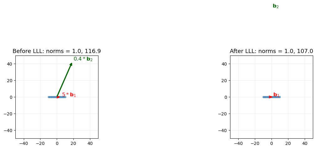
../_images/f32267a580617b03f8be96423045bb157cad3baf766c7390e7b2060a08bba834.png

Original basis norms:  1.0000, 116.8674
Reduced basis norms:   1.0000, 107.0000
Hadamard ratio before: 0.9569
Hadamard ratio after:  1.0000

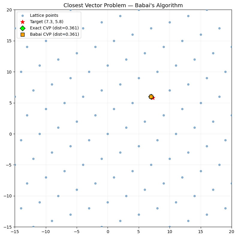
40.7 The Closest Vector Problem — Babai’s Algorithm#

Babai’s nearest-plane algorithm (1986) gives an approximate solution to CVP. Given a target \(\mathbf{t}\), it projects onto the Gram-Schmidt vectors to find a nearby lattice point.

With an LLL-reduced basis, Babai’s algorithm returns a vector \(\mathbf{v}\) with:

\[ \|\mathbf{v} - \mathbf{t}\| \le 2^{n/2} \cdot \text{dist}(\mathbf{t}, \mathcal{L}) \]

Show code cell source Hide code cell source

import numpy as np
import matplotlib.pyplot as plt
import math

def babai_cvp(basis, target):
    """Babai's nearest-plane algorithm for approximate CVP.

    Parameters
    ----------
    basis : ndarray, shape (n, m)
        LLL-reduced lattice basis (row vectors).
    target : ndarray, shape (m,)
        Target vector.

    Returns
    -------
    closest : ndarray
        Approximate closest lattice vector.
    """
    B = np.array(basis, dtype=float)
    t = np.array(target, dtype=float)
    n = B.shape[0]

    # Gram-Schmidt
    L = Lattice(B)
    Q, mu = L.gram_schmidt()

    # Round-off algorithm (Babai)
    b = t.copy()
    coeffs = np.zeros(n)
    for i in range(n - 1, -1, -1):
        qi_sq = np.dot(Q[i], Q[i])
        if qi_sq < 1e-14:
            coeffs[i] = 0
        else:
            coeffs[i] = round(np.dot(b, Q[i]) / qi_sq)
            b -= coeffs[i] * B[i]

    closest = np.zeros(B.shape[1])
    for i in range(n):
        closest += coeffs[i] * B[i]

    return closest

# Demonstrate CVP on a 2D lattice
B_cvp = np.array([[3, 1], [1, 4]], dtype=float)
B_cvp_lll = lll_reduce(B_cvp.copy())
target = np.array([7.3, 5.8])

closest_orig = babai_cvp(B_cvp, target)
closest_lll = babai_cvp(B_cvp_lll, target)

# Brute-force exact CVP for comparison
b1, b2 = B_cvp[0], B_cvp[1]
best_dist = float('inf')
exact_closest = None
for i in range(-20, 21):
    for j in range(-20, 21):
        v = i * b1 + j * b2
        d = np.linalg.norm(v - target)
        if d < best_dist:
            best_dist = d
            exact_closest = v.copy()

print(f"Target:              {target}")
print(f"Babai (original B):  {closest_orig}  dist = {float(np.linalg.norm(closest_orig - target)):.4f}")
print(f"Babai (LLL B):       {closest_lll}  dist = {float(np.linalg.norm(closest_lll - target)):.4f}")
print(f"Exact closest:       {exact_closest}  dist = {float(np.linalg.norm(exact_closest - target)):.4f}")

# Plot
fig, ax = plt.subplots(figsize=(8, 8))
pts = []
for i in range(-8, 9):
    for j in range(-8, 9):
        pt = i * b1 + j * b2
        if abs(pt[0]) < 25 and abs(pt[1]) < 25:
            pts.append(pt)
pts = np.array(pts)

ax.scatter(pts[:, 0], pts[:, 1], c='steelblue', s=20, zorder=3, alpha=0.6, label='Lattice points')
ax.scatter(*target, c='red', s=100, marker='*', zorder=5, label=f'Target ({target[0]}, {target[1]})')
ax.scatter(*exact_closest, c='lime', s=80, marker='D', zorder=5, edgecolors='black',
           label=f'Exact CVP (dist={float(best_dist):.3f})')
ax.scatter(*closest_lll, c='orange', s=80, marker='s', zorder=5, edgecolors='black',
           label=f'Babai CVP (dist={float(np.linalg.norm(closest_lll - target)):.3f})')

# Draw line from target to closest
ax.plot([target[0], exact_closest[0]], [target[1], exact_closest[1]], 'g--', lw=1.5, alpha=0.7)

ax.set_xlim(-15, 20)
ax.set_ylim(-15, 20)
ax.set_aspect('equal')
ax.legend(fontsize=10, loc='upper left')
ax.set_title("Closest Vector Problem — Babai's Algorithm", fontsize=13)
ax.grid(True, alpha=0.2)
plt.tight_layout()
plt.savefig("cvp_babai.png", dpi=150, bbox_inches="tight")
plt.show()

Target:              [7.3 5.8]
Babai (original B):  [7. 6.]  dist = 0.3606
Babai (LLL B):       [7. 6.]  dist = 0.3606
Exact closest:       [7. 6.]  dist = 0.3606

../_images/d45faa61a43350419c3b645259e8c9fed953d642762d9d0569c4713713ae5d2f.png

40.8 LWE Encryption Scheme#

We implement a simplified version of Regev’s LWE-based encryption scheme. The scheme encrypts single bits.

Key generation: Choose secret \(\mathbf{s} \in \mathbb{Z}_q^n\). Generate random matrix \(A \in \mathbb{Z}_q^{m \times n}\) and error vector \(\mathbf{e} \leftarrow \chi^m\). Public key: \((A, \mathbf{b} = A\mathbf{s} + \mathbf{e} \bmod q)\). Secret key: \(\mathbf{s}\).

Encryption of bit \(\mu \in \{0, 1\}\): Choose random subset \(S \subset [m]\). Compute:

\[ \mathbf{u} = \sum_{i \in S} \mathbf{a}_i \bmod q, \qquad v = \sum_{i \in S} b_i + \mu \cdot \lfloor q/2 \rfloor \bmod q\]

Decryption: Compute \(d = v - \langle \mathbf{u}, \mathbf{s} \rangle \bmod q\). Output 0 if \(d\) is closer to 0 than to \(\lfloor q/2 \rfloor\), else output 1.

import numpy as np
import math

def lwe_keygen(n, m, q, sigma=1.0, rng=None):
    """Generate LWE key pair.

    Parameters
    ----------
    n : int - secret dimension
    m : int - number of samples
    q : int - modulus
    sigma : float - error standard deviation
    rng : numpy RandomState

    Returns
    -------
    pk : tuple (A, b) - public key
    sk : ndarray - secret key s
    """
    if rng is None:
        rng = np.random.RandomState(42)

    s = rng.randint(0, q, size=n)  # secret
    A = rng.randint(0, q, size=(m, n))  # random matrix
    e = np.round(rng.normal(0, sigma, size=m)).astype(int) % q  # error
    b = (A @ s + e) % q

    return (A, b), s

def lwe_encrypt(pk, bit, q, rng=None):
    """Encrypt a single bit using LWE.

    Parameters
    ----------
    pk : tuple (A, b) - public key
    bit : int, 0 or 1
    q : int - modulus
    rng : numpy RandomState

    Returns
    -------
    ct : tuple (u, v) - ciphertext
    """
    if rng is None:
        rng = np.random.RandomState()

    A, b = pk
    m = A.shape[0]

    # Choose random subset
    subset = rng.choice([0, 1], size=m)

    u = (subset @ A) % q
    v = (int(subset @ b) + bit * (q // 2)) % q

    return (u, v)

def lwe_decrypt(sk, ct, q):
    """Decrypt an LWE ciphertext.

    Parameters
    ----------
    sk : ndarray - secret key s
    ct : tuple (u, v) - ciphertext
    q : int - modulus

    Returns
    -------
    bit : int, 0 or 1
    """
    u, v = ct
    d = (v - int(u @ sk)) % q

    # d should be close to 0 (for bit=0) or close to q//2 (for bit=1)
    if abs(d - q // 2) < q // 4:
        return 1
    elif d < q // 4 or d > 3 * q // 4:
        return 0
    else:
        # Ambiguous — treat as closest
        return 1 if abs(d - q // 2) < min(d, q - d) else 0

# Demo
n, m, q = 16, 64, 97
sigma = 1.5
rng = np.random.RandomState(2026)

pk, sk = lwe_keygen(n, m, q, sigma=sigma, rng=rng)
A, b = pk

print(f"Parameters: n={n}, m={m}, q={q}, sigma={sigma}")
print(f"Secret key s: {sk}")
print(f"Matrix A shape: {A.shape}")
print(f"Public vector b shape: {b.shape}")
print()

# Encrypt and decrypt several bits
test_bits = [0, 1, 1, 0, 1, 0, 0, 1]
print("Bit | Encrypted (u norm, v) | Decrypted | Correct?")
print("-" * 55)
all_correct = True
for i, bit in enumerate(test_bits):
    ct = lwe_encrypt(pk, bit, q, rng=np.random.RandomState(100 + i))
    dec = lwe_decrypt(sk, ct, q)
    correct = dec == bit
    all_correct = all_correct and correct
    print(f"  {bit} |     ({float(np.linalg.norm(ct[0])):.1f}, {int(ct[1]):3d})      |     {dec}     |   {correct}")

print(f"\nAll correct: {all_correct}")

Parameters: n=16, m=64, q=97, sigma=1.5
Secret key s: [ 1  6 26 56 77 77 29 28 51 69 76 28  2 54 77 27]
Matrix A shape: (64, 16)
Public vector b shape: (64,)

Bit | Encrypted (u norm, v) | Decrypted | Correct?
-------------------------------------------------------
  0 |     (270.8,  71)      |     0     |   True
  1 |     (241.1,  45)      |     1     |   True
  1 |     (193.5,  54)      |     1     |   True
  0 |     (247.2,  37)      |     0     |   True
  1 |     (221.5,  85)      |     1     |   True
  0 |     (240.5,  81)      |     0     |   True
  0 |     (261.2,   1)      |     0     |   True
  1 |     (218.8,  43)      |     1     |   True

All correct: True

40.9 LWE Error Distribution#

Visualization

The security of LWE depends critically on the error distribution. We visualize the discrete Gaussian errors and show how they affect the relationship between \(\mathbf{b}\) and \(A\mathbf{s}\).

../_images/d6230434c6f443170b1588acbc3ef3cbcfff925500a1d4d6bde9845ca4cc2a3f.png

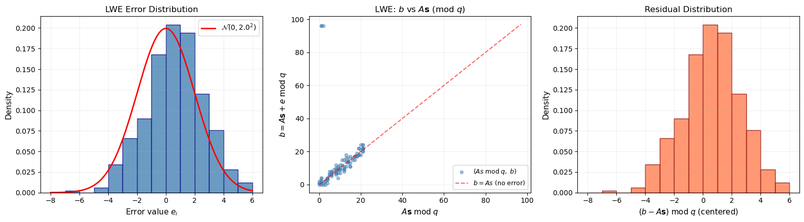
Error std dev (true): 2.0
Error std dev (measured): 2.002
Error range: [-7, 5]

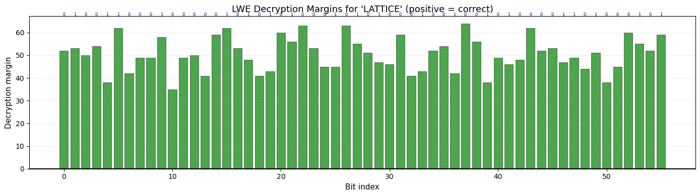
40.10 LWE Encryption — Bit-by-Bit Demo#

We encrypt a short binary message and visualize the decryption margin — how far each ciphertext’s decryption value is from the decision boundary.

Show code cell source Hide code cell source

import numpy as np
import matplotlib.pyplot as plt
import math

n, m, q = 32, 128, 257
sigma = 2.0
rng_kg = np.random.RandomState(42)
pk, sk = lwe_keygen(n, m, q, sigma=sigma, rng=rng_kg)

# Encrypt the ASCII message "LATTICE"
message = "LATTICE"
bits = []
for ch in message:
    for i in range(7, -1, -1):
        bits.append((ord(ch) >> i) & 1)

print(f"Message: '{message}'")
print(f"Bits ({len(bits)}): {''.join(map(str, bits))}")

# Encrypt each bit and track decryption margins
decrypted_bits = []
margins = []
for i, bit in enumerate(bits):
    ct = lwe_encrypt(pk, bit, q, rng=np.random.RandomState(1000 + i))
    u, v = ct
    d = (v - int(u @ sk)) % q
    # Centered
    d_centered = d if d <= q // 2 else d - q
    margin = abs(d_centered) - q // 4 if bit == 0 else abs(abs(d_centered) - q // 2) - q // 4
    dec = lwe_decrypt(sk, ct, q)
    decrypted_bits.append(dec)
    # Margin: positive = correct side of threshold
    if bit == 0:
        margins.append(q // 4 - min(d, q - d))
    else:
        margins.append(q // 4 - abs(d - q // 2))

# Reconstruct message
dec_chars = []
for i in range(0, len(decrypted_bits), 8):
    byte_bits = decrypted_bits[i:i+8]
    val = sum(b << (7 - j) for j, b in enumerate(byte_bits))
    dec_chars.append(chr(val))
recovered = ''.join(dec_chars)

print(f"Decrypted: '{recovered}'")
print(f"Match: {recovered == message}")

# Plot margins
fig, ax = plt.subplots(figsize=(14, 4))
colors = ['green' if m > 0 else 'red' for m in margins]
ax.bar(range(len(margins)), margins, color=colors, alpha=0.7, edgecolor='black', linewidth=0.5)
ax.axhline(y=0, color='black', lw=1.5)
ax.set_xlabel('Bit index', fontsize=11)
ax.set_ylabel('Decryption margin', fontsize=11)
ax.set_title(f"LWE Decryption Margins for '{message}' (positive = correct)", fontsize=13)
ax.grid(True, axis='y', alpha=0.2)

# Annotate original bits on top
for i, bit in enumerate(bits):
    ax.text(i, max(margins) * 1.05, str(bit), ha='center', fontsize=6, color='navy')

plt.tight_layout()
plt.savefig("lwe_decryption_margins.png", dpi=150, bbox_inches="tight")
plt.show()

Message: 'LATTICE'
Bits (56): 01001100010000010101010001010100010010010100001101000101
Decrypted: 'LATTICE'
Match: True

../_images/b9f423a4eb758b608b2c02157e640bb13e17492a6b230d13047a9df6d90c3212.png

40.11 SVP Approximation Quality of LLL#

We measure how well LLL approximates the shortest vector as a function of lattice dimension. For small dimensions we can compute the exact SVP by enumeration and compare with the LLL output.

Computational note

Exact SVP enumeration is exponential in the dimension. We restrict to dimensions 2–6 for tractability.

Show code cell source Hide code cell source

import numpy as np
import matplotlib.pyplot as plt
import math

def enumerate_svp(basis, search_radius=10):
    """Brute-force SVP for small lattices."""
    n = basis.shape[0]
    best_norm = float('inf')
    best_vec = None

    # Generate all integer combinations within search_radius
    ranges = [range(-search_radius, search_radius + 1)] * n

    def recurse(depth, coeffs):
        nonlocal best_norm, best_vec
        if depth == n:
            if all(c == 0 for c in coeffs):
                return
            v = sum(c * basis[i] for i, c in enumerate(coeffs))
            norm_v = np.linalg.norm(v)
            if norm_v < best_norm:
                best_norm = norm_v
                best_vec = v.copy()
            return
        for c in range(-search_radius, search_radius + 1):
            recurse(depth + 1, coeffs + [c])

    recurse(0, [])
    return best_vec, best_norm

rng = np.random.RandomState(2026)
dims = [2, 3, 4, 5]
n_trials = 15
approx_ratios = {d: [] for d in dims}

for dim in dims:
    for _ in range(n_trials):
        # Random integer basis
        B = rng.randint(-10, 11, size=(dim, dim)).astype(float)
        while abs(np.linalg.det(B)) < 1.0:
            B = rng.randint(-10, 11, size=(dim, dim)).astype(float)

        # LLL
        B_lll = lll_reduce(B.copy())
        lll_shortest = np.linalg.norm(B_lll[0])

        # Exact SVP
        sr = 8 if dim <= 4 else 5
        _, exact_shortest = enumerate_svp(B, search_radius=sr)

        if exact_shortest > 1e-10:
            ratio = lll_shortest / exact_shortest
            approx_ratios[dim].append(ratio)

fig, ax = plt.subplots(figsize=(10, 5))
positions = range(len(dims))
bp_data = [approx_ratios[d] for d in dims]
bp = ax.boxplot(bp_data, positions=positions, widths=0.5, patch_artist=True)

colors = ['#3498db', '#2ecc71', '#e67e22', '#e74c3c']
for patch, color in zip(bp['boxes'], colors):
    patch.set_facecolor(color)
    patch.set_alpha(0.7)

# Theoretical bound: 2^{(n-1)/2}
theoretical = [2**((d-1)/2) for d in dims]
ax.plot(positions, theoretical, 'k--', lw=2, marker='D', markersize=8,
        label=r'Theoretical bound $2^{(n-1)/2}$')

ax.set_xticks(positions)
ax.set_xticklabels([str(d) for d in dims])
ax.set_xlabel('Lattice dimension $n$', fontsize=12)
ax.set_ylabel(r'$\|\mathbf{b}_1^{LLL}\| / \lambda_1$', fontsize=12)
ax.set_title('LLL Approximation Ratio vs. Dimension', fontsize=13)
ax.legend(fontsize=11)
ax.grid(True, axis='y', alpha=0.3)
ax.set_ylim(0.8, max(theoretical) * 1.3)

plt.tight_layout()
plt.savefig("svp_approximation.png", dpi=150, bbox_inches="tight")
plt.show()

for d in dims:
    ratios = approx_ratios[d]
    print(f"Dim {d}: mean ratio = {float(np.mean(ratios)):.3f}, "
          f"max = {float(np.max(ratios)):.3f}, "
          f"bound = {float(2**((d-1)/2)):.3f}")

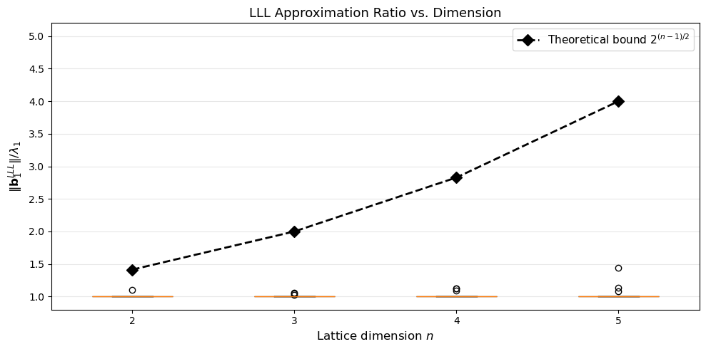
../_images/7add9df5d52237923d5768393789559b5c470a8f10430e6a23507d920e633bb1.png

Dim 2: mean ratio = 1.007, max = 1.098, bound = 1.414
Dim 3: mean ratio = 1.008, max = 1.055, bound = 2.000
Dim 4: mean ratio = 1.023, max = 1.129, bound = 2.828
Dim 5: mean ratio = 1.044, max = 1.442, bound = 4.000

40.12 LWE Security: Effect of Parameters#

The security of LWE depends on the relationship between the dimension \(n\), modulus \(q\), and error rate \(\sigma/q\). We explore how decryption error rates change with these parameters.

Show code cell source Hide code cell source

import numpy as np
import matplotlib.pyplot as plt
import math

def lwe_error_rate(n, m, q, sigma, n_trials=500, rng_seed=42):
    """Estimate LWE decryption error rate."""
    rng = np.random.RandomState(rng_seed)
    pk, sk = lwe_keygen(n, m, q, sigma=sigma, rng=rng)

    errors = 0
    for i in range(n_trials):
        bit = rng.randint(0, 2)
        ct = lwe_encrypt(pk, bit, q, rng=np.random.RandomState(rng_seed + 1000 + i))
        dec = lwe_decrypt(sk, ct, q)
        if dec != bit:
            errors += 1
    return errors / n_trials

# Experiment 1: vary sigma for fixed n, q
sigmas = np.arange(0.5, 12.1, 0.5)
n_fix, m_fix, q_fix = 32, 128, 257

err_rates_sigma = []
for sig in sigmas:
    rate = lwe_error_rate(n_fix, m_fix, q_fix, sig, n_trials=400)
    err_rates_sigma.append(rate)

# Experiment 2: vary q for fixed n, sigma
qs = [31, 53, 97, 127, 199, 257, 509, 1021]
sigma_fix = 2.0

err_rates_q = []
for qi in qs:
    rate = lwe_error_rate(n_fix, m_fix, qi, sigma_fix, n_trials=400)
    err_rates_q.append(rate)

fig, axes = plt.subplots(1, 2, figsize=(14, 5))

axes[0].plot(sigmas, err_rates_sigma, 'o-', color='steelblue', lw=2, markersize=5)
axes[0].axhline(y=0.01, color='red', ls='--', lw=1.5, alpha=0.6, label='1% error threshold')
axes[0].set_xlabel(r'Error std dev $\sigma$', fontsize=12)
axes[0].set_ylabel('Decryption error rate', fontsize=12)
axes[0].set_title(r'Error Rate vs. $\sigma$' + f' (n={n_fix}, q={q_fix})', fontsize=13)
axes[0].legend(fontsize=10)
axes[0].grid(True, alpha=0.3)
axes[0].set_ylim(-0.02, 0.55)

axes[1].plot(qs, err_rates_q, 's-', color='coral', lw=2, markersize=6)
axes[1].axhline(y=0.01, color='red', ls='--', lw=1.5, alpha=0.6, label='1% error threshold')
axes[1].set_xlabel(r'Modulus $q$', fontsize=12)
axes[1].set_ylabel('Decryption error rate', fontsize=12)
axes[1].set_title(r'Error Rate vs. $q$' + f' (n={n_fix}, ' + r'$\sigma$' + f'={sigma_fix})', fontsize=13)
axes[1].legend(fontsize=10)
axes[1].grid(True, alpha=0.3)
axes[1].set_ylim(-0.02, 0.55)

plt.tight_layout()
plt.savefig("lwe_security_params.png", dpi=150, bbox_inches="tight")
plt.show()

print("Sigma sweep (key results):")
for sig, rate in zip(sigmas, err_rates_sigma):
    if rate > 0:
        print(f"  sigma={float(sig):.1f}: error rate = {float(rate):.3f}")
        break
else:
    print("  All error rates are 0 in sigma sweep")

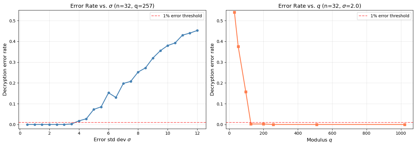
../_images/fd238cdb8fb512851ef03bcb3ddc2194209eed47e4615c203b96147c03997a5d.png

Sigma sweep (key results):
  sigma=3.5: error rate = 0.003

40.13 3D Lattice Visualization#

We visualize a 3D lattice and its LLL-reduced basis to build geometric intuition.

../_images/6f1d4e64652b95188f7c56c74f9739e2936c116abb3492ae3117146fe0eaa821.png

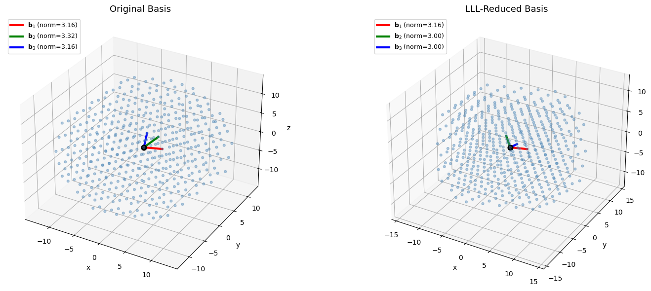
Original basis norms: ['3.162', '3.317', '3.162']
Reduced basis norms:  ['3.162', '3.000', '3.000']
Hadamard ratio before: 0.8587
Hadamard ratio after:  0.9036

40.14 Gram-Schmidt Orthogonalization Visualized#

The Gram-Schmidt process is fundamental to both LLL and Babai’s CVP algorithm. We visualize how the GSO transforms a 2D basis.

<>:24: SyntaxWarning: invalid escape sequence '\c'
<>:45: SyntaxWarning: invalid escape sequence '\m'
<>:49: SyntaxWarning: invalid escape sequence '\c'
<>:24: SyntaxWarning: invalid escape sequence '\c'
<>:45: SyntaxWarning: invalid escape sequence '\m'
<>:49: SyntaxWarning: invalid escape sequence '\c'
/var/folders/z7/wp7m8p7x1250jzvklw5z24mm0000gn/T/ipykernel_6168/2382662601.py:24: SyntaxWarning: invalid escape sequence '\c'
  ax.set_title(f'Original Basis (angle = {float(angle):.1f}$^\circ$)', fontsize=13)
/var/folders/z7/wp7m8p7x1250jzvklw5z24mm0000gn/T/ipykernel_6168/2382662601.py:45: SyntaxWarning: invalid escape sequence '\m'
  ax.text(proj[0]-0.5, proj[1]-0.4, f'$\mu_{{2,1}} = {float(mu[1,0]):.3f}$', fontsize=11, color='purple')
/var/folders/z7/wp7m8p7x1250jzvklw5z24mm0000gn/T/ipykernel_6168/2382662601.py:49: SyntaxWarning: invalid escape sequence '\c'
  ax.set_title(f'Gram-Schmidt Basis (angle = {float(angle_gs):.1f}$^\circ$)', fontsize=13)

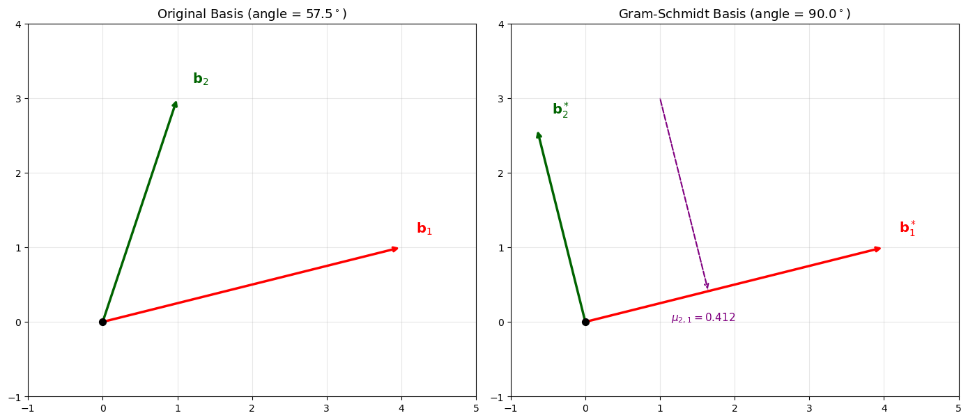
../_images/38904d5bf5a4c1fb3b5dbc5c2eefbb4f133c830c58d2768902ff080a0ce994e3.png

mu[1,0] = 0.411765
Verification: b2 = b2* + mu[1,0]*b1* = [1. 3.] (should be [1. 3.])

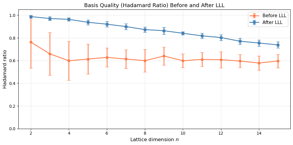
40.15 LLL Reduction: Hadamard Ratio Across Dimensions#

We measure how the Hadamard ratio (basis quality) improves after LLL reduction, as a function of lattice dimension.

../_images/aba187726f7084381db6be10962045d7b86a0d95ebb61f51890f5d3346ef98a1.png

Dimension | Mean HR Before | Mean HR After | Improvement
----------------------------------------------------------
   |     0.7628     |    0.9880    |  1.30x
   |     0.6597     |    0.9711    |  1.47x
   |     0.5984     |    0.9637    |  1.61x
   |     0.6136     |    0.9378    |  1.53x
   |     0.6284     |    0.9213    |  1.47x
   |     0.6138     |    0.9000    |  1.47x
   |     0.5996     |    0.8734    |  1.46x
   |     0.6406     |    0.8633    |  1.35x
   |     0.5991     |    0.8410    |  1.40x
   |     0.6109     |    0.8185    |  1.34x
   |     0.6081     |    0.8035    |  1.32x
   |     0.5965     |    0.7707    |  1.29x
   |     0.5789     |    0.7552    |  1.30x
   |     0.5963     |    0.7383    |  1.24x

40.16 Connection: CVP and LWE#

LWE can be viewed as a CVP instance. Given \((A, \mathbf{b} = A\mathbf{s} + \mathbf{e})\), consider the lattice generated by the rows of \(A\) (mod \(q\)). The vector \(\mathbf{b}\) is a lattice point (namely \(A\mathbf{s}\)) plus a small error \(\mathbf{e}\). Solving LWE is equivalent to solving CVP on this lattice with target \(\mathbf{b}\).

Reduction chain

The security of lattice-based cryptography rests on a chain of reductions:

\[ \text{worst-case GapSVP} \le_p \text{LWE} \le_p \text{CVP on } q\text{-ary lattice}\]

Breaking LWE \(\Rightarrow\) solving CVP \(\Rightarrow\) solving approximate SVP in the worst case.

Show code cell source Hide code cell source

import numpy as np
import matplotlib.pyplot as plt
import math

# Show that LWE is a CVP instance in 2D
rng = np.random.RandomState(42)
q = 23
n_lwe = 2

# Secret and samples
s = rng.randint(0, q, size=n_lwe)
A = rng.randint(0, q, size=(5, n_lwe))
e = np.round(rng.normal(0, 1.0, size=5)).astype(int)
b = (A @ s + e) % q

# Build the q-ary lattice: points of the form A*x mod q
fig, ax = plt.subplots(figsize=(8, 8))

# Lattice points: all A*x mod q for integer x
lattice_pts = set()
for x0 in range(q):
    for x1 in range(q):
        x_vec = np.array([x0, x1])
        for row_idx in range(A.shape[0]):
            pt = tuple((A[row_idx] * x_vec[0]) % q)
            lattice_pts.add(pt)

# More complete: generate all vectors in the lattice (column span of A mod q)
lattice_pts = []
for x0 in range(q):
    for x1 in range(q):
        pt = (A[0] * x0 + A[1] * x1) % q
        lattice_pts.append(pt)
lattice_pts = np.array(list(set(map(tuple, lattice_pts))))

ax.scatter(lattice_pts[:, 0], lattice_pts[:, 1], c='steelblue', s=20, alpha=0.5,
           label=r'Lattice points ($A\mathbf{x} \; \mathrm{mod} \; q$)')

# Target (b values from first two samples)
for i in range(min(3, len(b))):
    target_2d = np.array([b[i] % q, b[(i+1) % len(b)] % q])
    ax.scatter(*target_2d, c='red', s=100, marker='*', zorder=5)

# The actual A*s mod q (closest lattice point)
As_mod_q = (A @ s) % q
for i in range(min(3, len(As_mod_q))):
    actual_2d = np.array([As_mod_q[i] % q, As_mod_q[(i+1) % len(As_mod_q)] % q])
    ax.scatter(*actual_2d, c='lime', s=80, marker='D', zorder=5, edgecolors='black')

ax.set_xlabel(r'$x_1$', fontsize=12)
ax.set_ylabel(r'$x_2$', fontsize=12)
ax.set_title(r'LWE as CVP: Target $\mathbf{b}$ (stars) Near Lattice Point $A\mathbf{s}$ (diamonds)', fontsize=12)
ax.set_xlim(-1, q)
ax.set_ylim(-1, q)
ax.grid(True, alpha=0.2)
ax.legend(fontsize=10)

plt.tight_layout()
plt.savefig("lwe_as_cvp.png", dpi=150, bbox_inches="tight")
plt.show()

print(f"Secret s = {s}")
print(f"A*s mod q = {(A @ s) % q}")
print(f"b = A*s+e mod q = {b}")
print(f"Error e = {e}")

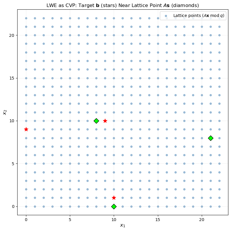
../_images/6346b235aa640839691d84e4fdd23557e915771a4b3a9710222fece2f95b281c.png

Secret s = [ 6 19]
A*s mod q = [21  8 10  0  3]
b = A*s+e mod q = [ 0  9 10  1  3]
Error e = [2 1 0 1 0]

40.17 Exercises#

Exercise 1: Implementing Gaussian Heuristic

The Gaussian heuristic predicts that the shortest vector in a random \(n\)-dimensional lattice of determinant \(\det(\mathcal{L})\) has length approximately:

\[ \lambda_1 \approx \sqrt{\frac{n}{2\pi e}} \cdot (\det \mathcal{L})^{1/n}\]

Generate random lattices of dimensions 2 through 8, compute the exact shortest vector (by enumeration for small dimensions), and compare with the Gaussian heuristic prediction. Plot the ratio \(\lambda_1^{\text{actual}} / \lambda_1^{\text{predicted}}\).

Hint

Use enumerate_svp for dimensions up to 5, and lll_reduce as an upper bound for larger dimensions. The determinant of the lattice is abs(det(B)).

Exercise 2: LLL with Different \(\delta\) Parameters

The LLL algorithm has a parameter \(\delta \in (1/4, 1]\) controlling the quality/speed tradeoff. Implement an experiment that runs LLL with \(\delta \in \{0.5, 0.75, 0.99\}\) on random 10-dimensional lattices and compares: (a) the Hadamard ratio of the output, (b) the norm of the first basis vector, and (c) the number of swap operations.

Hint

Modify lll_reduce to count swaps. A larger \(\delta\) produces a better basis but requires more swaps.

Exercise 3: LWE Parameter Selection

For the LWE encryption scheme, find the largest \(\sigma\) such that the decryption error rate remains below 1% for parameters \(n = 64\), \(m = 256\), \(q = 521\). Then increase \(n\) to 128 (keeping \(q = 521\)) and find the new maximum \(\sigma\). Explain the relationship.

Hint

Use binary search on \(\sigma\) with lwe_error_rate. The maximum tolerable \(\sigma\) grows roughly as \(q / (4\sqrt{m})\) — more samples (larger \(m\)) means more accumulated noise.

Exercise 4: Knapsack Problem via Lattice Reduction

The subset-sum (knapsack) problem can be reduced to SVP. Given weights \(w_1, \ldots, w_n\) and a target \(S = \sum_{i \in T} w_i\), construct the lattice with basis:

\[\begin{split} B = \begin{pmatrix} 2 & 0 & \cdots & 0 & w_1 \\ 0 & 2 & \cdots & 0 & w_2 \\ \vdots & & \ddots & & \vdots \\ 0 & 0 & \cdots & 2 & w_n \\ 1 & 1 & \cdots & 1 & S \end{pmatrix}\end{split}\]

Apply LLL to this lattice and check if the shortest vector reveals the subset \(T\). Demonstrate with a small instance (\(n = 8\), random weights).

Hint

In the shortest vector, the last coordinate should be 0 (or close to 0), and the first \(n\) coordinates should be \(\pm 1\), encoding the subset membership: \(+1\) means \(i \in T\), \(-1\) means \(i \notin T\).

Exercise 5: Ring-LWE Toy Implementation

Implement a toy Ring-LWE scheme over \(R_q = \mathbb{Z}_q[x]/(x^n + 1)\) with \(n = 8\), \(q = 257\). Polynomial multiplication in \(R_q\) is multiplication modulo \(x^n + 1\) and reduction modulo \(q\). Implement ring_lwe_keygen, ring_lwe_encrypt, and ring_lwe_decrypt, and demonstrate correct encryption/decryption.

Hint

Represent polynomials as NumPy arrays of length \(n\). Use np.polymul followed by reduction modulo \(x^n + 1\) (which maps \(x^n \to -1\), \(x^{n+1} \to -x\), etc.). Alternatively, implement negacyclic convolution directly.

40.18 Summary#

In this chapter we studied the foundational lattice problems underlying modern post-quantum cryptography:

Lattices are discrete subgroups of \(\mathbb{R}^n\), generated by integer combinations of basis vectors. Different bases can generate the same lattice but vary dramatically in quality.
SVP (Shortest Vector Problem) asks to find the shortest nonzero lattice vector. It is NP-hard to solve exactly and believed hard to approximate within polynomial factors.
CVP (Closest Vector Problem) asks to find the lattice point nearest to a given target. CVP is at least as hard as SVP.
LWE (Learning With Errors) is a problem of solving noisy linear equations modulo \(q\). Regev (2005) proved that solving LWE is as hard as solving worst-case lattice problems, providing a strong theoretical foundation for cryptographic constructions.
LLL reduction is the key algorithmic tool: it runs in polynomial time and produces a basis whose shortest vector is within an exponential factor of optimal. Despite this approximation gap, LLL is essential for both attacks and constructions.
LWE-based encryption adds small noise to linear equations, making them unsolvable without the secret key. The tradeoff between noise magnitude and decryption correctness is central to parameter selection.

The NIST post-quantum standards (ML-KEM/Kyber, ML-DSA/Dilithium) are built on Module-LWE, combining the security of LWE with the efficiency of ring structure.

40.19 References#

Ajtai, M. (1996). “Generating Hard Instances of Lattice Problems.” Proceedings of the 28th Annual ACM Symposium on Theory of Computing (STOC), pp. 99–108. doi:10.1145/237814.237838
Regev, O. (2005). “On Lattices, Learning with Errors, Random Linear Codes, and Cryptography.” Proceedings of the 37th Annual ACM Symposium on Theory of Computing (STOC), pp. 84–93. doi:10.1145/1060590.1060603
Lenstra, A.K., Lenstra, H.W., and Lovász, L. (1982). “Factoring Polynomials with Rational Coefficients.” Mathematische Annalen, 261, pp. 515–534. doi:10.1007/BF01457454
Micciancio, D. and Regev, O. (2009). “Lattice-based Cryptography.” In Post-Quantum Cryptography, Springer, pp. 147–191. doi:10.1007/978-3-540-88702-7_5
Peikert, C. (2016). “A Decade of Lattice Cryptography.” Foundations and Trends in Theoretical Computer Science, 10(4), pp. 283–424. doi:10.1561/0400000074
Lyubashevsky, V., Peikert, C., and Regev, O. (2010). “On Ideal Lattices and Learning with Errors over Rings.” EUROCRYPT 2010, LNCS 6110, pp. 1–23.
Babai, L. (1986). “On Lovász’ Lattice Reduction and the Nearest Lattice Point Problem.” Combinatorica, 6(1), pp. 1–13. doi:10.1007/BF02579403
NIST (2024). “Module-Lattice-Based Key-Encapsulation Mechanism Standard (FIPS 203).” https://csrc.nist.gov/pubs/fips/203/final

Chapter 40: Lattice Problems — SVP, CVP, and LWE

Contents

Chapter 40: Lattice Problems — SVP, CVP, and LWE#

40.1 Introduction and Historical Context#

40.2 Definitions#

40.2.1 Lattice#

40.2.2 Shortest Vector Problem (SVP)#

40.2.3 Closest Vector Problem (CVP)#

40.2.4 Learning With Errors (LWE)#

40.2.5 Ring-LWE and Module-LWE#

40.2.6 Ajtai’s Reduction (Conceptual)#

40.3 Lattice Class with Gram-Schmidt and LLL Reduction#

40.4 LLL Basis Reduction Algorithm#

40.5 Visualizing 2D Lattices#

40.6 LLL Reduction: Before and After#

40.7 The Closest Vector Problem — Babai’s Algorithm#

40.8 LWE Encryption Scheme#

40.9 LWE Error Distribution#

40.10 LWE Encryption — Bit-by-Bit Demo#

40.11 SVP Approximation Quality of LLL#

40.12 LWE Security: Effect of Parameters#

40.13 3D Lattice Visualization#

40.14 Gram-Schmidt Orthogonalization Visualized#

40.15 LLL Reduction: Hadamard Ratio Across Dimensions#

40.16 Connection: CVP and LWE#

40.17 Exercises#

40.18 Summary#

40.19 References#