
Chapter 3: Frequency Analysis#
3.1 Introduction: Al-Kindi’s Revolution#
In the ninth century, the Arab polymath Abu Yusuf Ya’qub ibn Ishaq al-Kindi (c. 801–873 AD) composed what is widely regarded as the earliest known treatise on cryptanalysis: Risalah fi Istikhraj al-Mu’amma (“A Manuscript on Deciphering Cryptographic Messages”). Written around 850 AD in Baghdad during the golden age of Islamic scholarship, this work laid the intellectual foundation for a technique that would dominate codebreaking for the next millennium: frequency analysis.
Al-Kindi’s key insight was elegantly simple yet profoundly powerful. He observed that every natural language exhibits a characteristic statistical fingerprint – certain letters appear far more often than others, and this pattern is remarkably stable across large bodies of text. In his own words:
“One way to solve an encrypted message, if we know its language, is to find a different plaintext of the same language long enough to fill one sheet or so, and then we count the occurrences of each letter. We call the most frequently occurring letter the ‘first’, the next most frequently occurring letter the ‘second’, the following most frequently occurring letter the ‘third’, and so on, until we account for all the different letters in the plaintext sample.
Then we look at the cipher text we want to solve and we also classify its symbols. We find the most occurring symbol and change it to the form of the ‘first’ letter of the plaintext sample, the next most common symbol is changed to the form of the ‘second’ letter, and the following most common symbol is changed to the form of the ‘third’ letter, and so on, until we account for all symbols of the cryptogram we want to solve.”
– Al-Kindi, Risalah fi Istikhraj al-Mu’amma (c. 850 AD)
This procedure – counting letter occurrences in ciphertext and matching them to the known frequency profile of the underlying language – gave cryptanalysts a systematic weapon against monoalphabetic substitution ciphers. Before Al-Kindi, breaking such ciphers relied on guesswork, divine inspiration, or brute force. After Al-Kindi, it became a matter of patient statistical bookkeeping.
For roughly a thousand years, from the medieval Arab world through Renaissance Europe and into the early modern period, frequency analysis remained the primary tool of the codebreaker. It was not until the development of polyalphabetic ciphers (Chapter 5) that cryptographers found a way to resist this attack – and even then, frequency analysis adapted and persisted through techniques such as the Kasiski examination and the index of coincidence.
Tip
Statistics as a cryptanalytic weapon. Al-Kindi’s revolution was not merely a clever trick; it was the recognition that mathematics – specifically, the statistical structure of language – could be weaponized against secret communication. This idea remains central to modern cryptanalysis: every cipher must resist statistical attacks, or it is broken.
3.2 Formal Definitions#
We now formalize the concepts underlying frequency analysis. Throughout this chapter, we work with an alphabet \(\mathcal{A} = \{a, b, c, \ldots, z\}\) of size \(n = 26\) (the standard English/Latin alphabet).
Danger
Frequency analysis fails on short texts. The law of large numbers guarantees that letter frequencies converge to their expected values as text length \(N \to \infty\). For short texts (\(N < 100\)), the observed frequencies can deviate wildly from the expected distribution, making frequency analysis unreliable. As a rule of thumb, at least several hundred characters are needed for frequency-based attacks to succeed consistently.
import numpy as np
import matplotlib.pyplot as plt
%matplotlib inline
import string
import re

# Standard English letter frequencies (from large corpus analysis)
# Stored in alphabetical order: a, b, c, ..., z
ENGLISH_FREQ = np.array([
    0.0817, 0.0129, 0.0278, 0.0425, 0.1270, 0.0223,  # a-f
    0.0202, 0.0609, 0.0697, 0.0015, 0.0077, 0.0403,  # g-l
    0.0241, 0.0675, 0.0751, 0.0193, 0.0010, 0.0599,  # m-r
    0.0633, 0.0906, 0.0276, 0.0098, 0.0236, 0.0015,  # s-x
    0.0197, 0.0007                                     # y-z
])

ENGLISH_LETTERS = list(string.ascii_lowercase)


class FrequencyAnalyzer:
    """
    Compute and compare letter frequency distributions.

    Parameters
    ----------
    alphabet : list
        The alphabet to analyze (default: English lowercase a-z).
    """

    def __init__(self, alphabet=None):
        self.alphabet = alphabet or ENGLISH_LETTERS
        self.n = len(self.alphabet)

    def clean_text(self, text):
        """Remove non-alphabet characters and convert to lowercase."""
        return re.sub(r'[^a-z]', '', text.lower())

    def compute_frequency(self, text):
        """
        Compute letter frequency vector for a given text.

        Parameters
        ----------
        text : str
            Input text (will be cleaned automatically).

        Returns
        -------
        np.ndarray
            Frequency vector of length self.n.
        """
        cleaned = self.clean_text(text)
        if len(cleaned) == 0:
            return np.zeros(self.n)
        counts = np.array([cleaned.count(c) for c in self.alphabet])
        return counts / len(cleaned)

    def euclidean_distance(self, freq1, freq2):
        """Compute Euclidean distance between two frequency vectors."""
        return np.sqrt(np.sum((freq1 - freq2)**2))

    def chi_squared(self, observed_freq, expected_freq):
        """
        Compute chi-squared statistic between observed and expected frequencies.

        Only sums over positions where expected_freq > 0 to avoid division by zero.
        """
        mask = expected_freq > 0
        return np.sum((observed_freq[mask] - expected_freq[mask])**2 / expected_freq[mask])

    def plot_frequency(self, freq, title='Letter Frequency Distribution', ax=None,
                       color='steelblue', reference_freq=None, figsize=(12, 5)):
        """
        Plot a frequency distribution as a bar chart.

        Parameters
        ----------
        freq : np.ndarray
            Frequency vector to plot.
        title : str
            Plot title.
        ax : matplotlib.axes.Axes or None
            Axes to plot on. If None, a new figure is created.
        color : str
            Bar color.
        reference_freq : np.ndarray or None
            If provided, overlay a reference distribution as red markers.
        figsize : tuple
            Figure size (width, height).

        Returns
        -------
        matplotlib.axes.Axes
        """
        if ax is None:
            fig, ax = plt.subplots(1, 1, figsize=figsize)
        x = np.arange(self.n)
        ax.bar(x, freq, color=color, alpha=0.8, label='Observed')
        if reference_freq is not None:
            ax.scatter(x, reference_freq, color='red', zorder=5, s=30, label='Expected (English)')
        ax.set_xticks(x)
        ax.set_xticklabels(self.alphabet, fontsize=9)
        ax.set_ylabel('Relative Frequency')
        ax.set_title(title)
        ax.set_xlim(-0.6, self.n - 0.4)
        if reference_freq is not None:
            ax.legend()
        return ax


# Quick demonstration
analyzer = FrequencyAnalyzer()
print(f'Alphabet size: {analyzer.n}')
print(f'English frequency vector sums to: {float(ENGLISH_FREQ.sum()):.4f}')
print(f'Most frequent English letter: {ENGLISH_LETTERS[np.argmax(ENGLISH_FREQ)]} ({float(ENGLISH_FREQ.max()):.4f})')
print(f'Least frequent English letter: {ENGLISH_LETTERS[np.argmin(ENGLISH_FREQ)]} ({float(ENGLISH_FREQ.min()):.4f})')
Alphabet size: 26
English frequency vector sums to: 0.9982
Most frequent English letter: e (0.1270)
Least frequent English letter: z (0.0007)
3.3 Breaking the Shift Cipher with Frequency Analysis#
The shift cipher (also called the Caesar cipher) encrypts a message by replacing each letter \(a_i\) with \(a_{(i+k) \bmod n}\), where \(k\) is the secret key and \(n = |\mathcal{A}|\). We now show that frequency analysis recovers \(k\) efficiently.
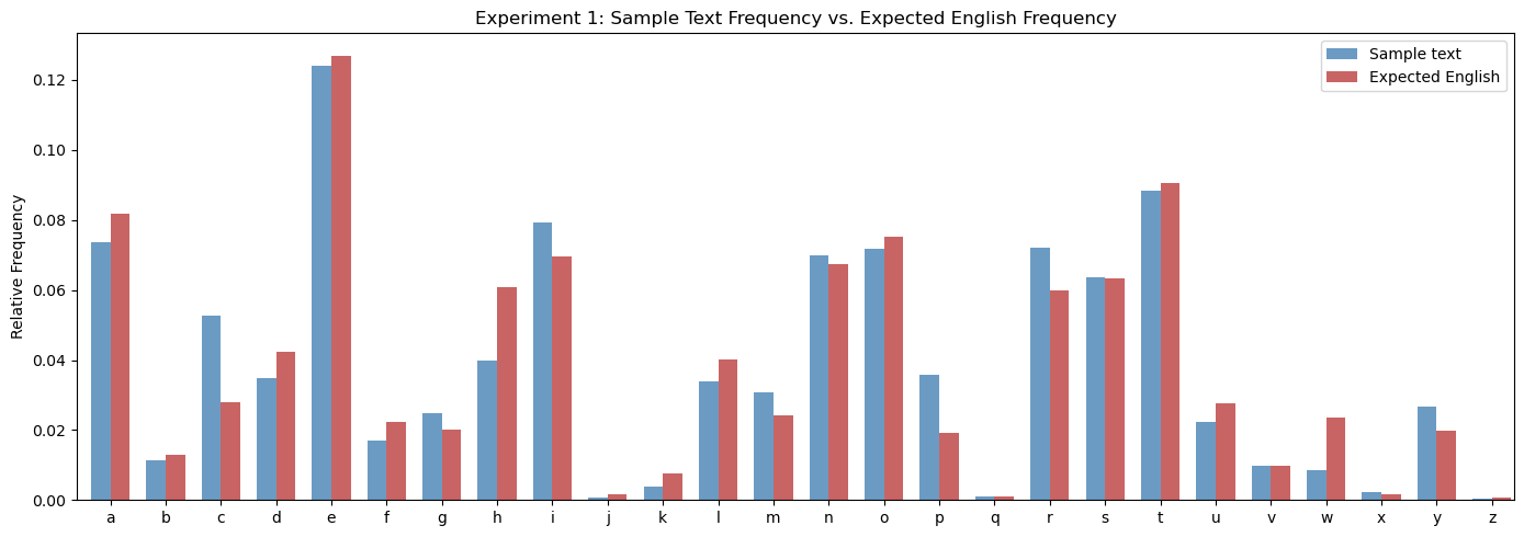
Experiment 1: Frequency Distribution of English Text#
We compute and plot the letter frequency distribution of a long English sample and compare it to the standard expected frequencies.
Show code cell source
import numpy as np
import matplotlib.pyplot as plt
%matplotlib inline
import string
import re

ENGLISH_FREQ = np.array([
    0.0817, 0.0129, 0.0278, 0.0425, 0.1270, 0.0223,
    0.0202, 0.0609, 0.0697, 0.0015, 0.0077, 0.0403,
    0.0241, 0.0675, 0.0751, 0.0193, 0.0010, 0.0599,
    0.0633, 0.0906, 0.0276, 0.0098, 0.0236, 0.0015,
    0.0197, 0.0007
])
ENGLISH_LETTERS = list(string.ascii_lowercase)

# A long English sample text (excerpt adapted from public domain sources)
sample_text = '''
Cryptography is the practice and study of techniques for secure communication in the
presence of adversarial behavior. More generally, cryptography is about constructing and
analyzing protocols that prevent third parties or the public from reading private messages.
Modern cryptography exists at the intersection of the disciplines of mathematics and
computer science and electrical engineering. Applications of cryptography include
electronic commerce, chip-based payment cards, digital currencies, computer passwords,
and military communications.

Cryptography prior to the modern age was effectively synonymous with encryption,
converting readable information to unintelligible nonsense text, which can only be read
by reversing the process. The originator of an encrypted message shares the decoding
technique only with intended recipients to preclude access from adversaries. The
cryptography literature often uses the names Alice and Bob to refer to the sender and
the intended recipient respectively. Since the development of rotor cipher machines in
World War I and the advent of computers in World War II, cryptography methods have
become increasingly complex and their applications more varied.

Modern cryptography is heavily based on mathematical theory and computer science
practice. Cryptographic algorithms are designed around computational hardness
assumptions, making such algorithms hard to break in actual practice by any adversary.
While it is theoretically possible to break into a well-designed system, it is infeasible
in actual practice to do so. Such schemes, if well designed, are therefore termed
computationally secure. There exist information-theoretically secure schemes that
provably cannot be broken even with unlimited computing power, but these schemes are
more difficult to use in practice than the best theoretically breakable but
computationally secure schemes.

The growth of cryptographic technology has raised a number of legal issues in the
information age. The potential for use as a tool for espionage and sedition has led many
governments to classify it as a weapon and to limit or even prohibit its use and export.
In some jurisdictions where the use of cryptography is legal, laws permit investigators
to compel the disclosure of encryption keys for documents relevant to an investigation.
Cryptography also plays a major role in digital rights management and copyright
infringement disputes with regard to digital media.

The first use of the term cryptograph as opposed to cryptogram was by the English
novelist William Makepeace Thackeray in his work from the eighteen forties. Before
the modern era, cryptography focused on message confidentiality through the encryption
of written messages converting them to apparent nonsense. Encryption attempted to ensure
secrecy in communications, such as those of spies, military leaders, and diplomats.
In recent decades the field has expanded beyond confidentiality concerns to include
techniques for message integrity checking, sender and receiver identity authentication,
digital signatures, interactive proofs, and secure computation, among others.
'''

def clean_text(text):
    return re.sub(r'[^a-z]', '', text.lower())

def compute_frequency(text):
    cleaned = clean_text(text)
    if len(cleaned) == 0:
        return np.zeros(26)
    counts = np.array([cleaned.count(c) for c in ENGLISH_LETTERS])
    return counts / len(cleaned)

# Compute frequencies of the sample
sample_freq = compute_frequency(sample_text)
cleaned_sample = clean_text(sample_text)
print(f'Sample length (cleaned): {len(cleaned_sample)} characters')
print(f'Euclidean distance from expected English: {float(np.sqrt(np.sum((sample_freq - ENGLISH_FREQ)**2))):.6f}')

# Plot comparison
fig, ax = plt.subplots(1, 1, figsize=(14, 5))
x = np.arange(26)
width = 0.35
ax.bar(x - width/2, sample_freq, width, color='steelblue', alpha=0.8, label='Sample text')
ax.bar(x + width/2, ENGLISH_FREQ, width, color='firebrick', alpha=0.7, label='Expected English')
ax.set_xticks(x)
ax.set_xticklabels(ENGLISH_LETTERS, fontsize=10)
ax.set_ylabel('Relative Frequency')
ax.set_title('Experiment 1: Sample Text Frequency vs. Expected English Frequency')
ax.legend()
ax.set_xlim(-0.6, 25.4)
plt.tight_layout()
plt.savefig('fig_ch03_exp1_frequency_comparison.png', dpi=150, bbox_inches='tight')
plt.show()
Sample length (cleaned): 2645 characters
Euclidean distance from expected English: 0.046797
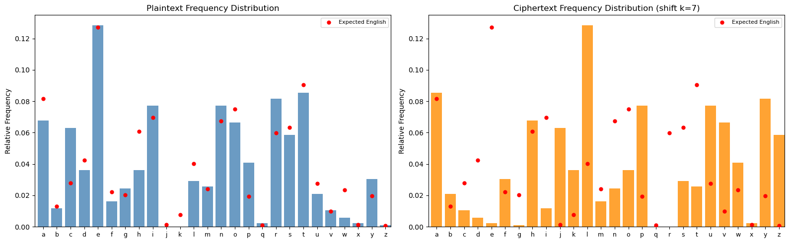
Experiment 2: Breaking a Shift Cipher#
We encrypt a text with shift key \(k = 7\), observe how the frequency distribution shifts, and then recover the key by testing all 26 possible shifts and selecting the one that minimizes the chi-squared statistic.
Show code cell source
import numpy as np
import matplotlib.pyplot as plt
%matplotlib inline
import string
import re

ENGLISH_FREQ = np.array([
    0.0817, 0.0129, 0.0278, 0.0425, 0.1270, 0.0223,
    0.0202, 0.0609, 0.0697, 0.0015, 0.0077, 0.0403,
    0.0241, 0.0675, 0.0751, 0.0193, 0.0010, 0.0599,
    0.0633, 0.0906, 0.0276, 0.0098, 0.0236, 0.0015,
    0.0197, 0.0007
])
ENGLISH_LETTERS = list(string.ascii_lowercase)

def clean_text(text):
    return re.sub(r'[^a-z]', '', text.lower())

def compute_frequency(text):
    cleaned = clean_text(text)
    if len(cleaned) == 0:
        return np.zeros(26)
    counts = np.array([cleaned.count(c) for c in ENGLISH_LETTERS])
    return counts / len(cleaned)

def chi_squared(observed, expected):
    mask = expected > 0
    return np.sum((observed[mask] - expected[mask])**2 / expected[mask])

def shift_encrypt(text, key):
    """Encrypt text using a shift cipher with the given key."""
    cleaned = clean_text(text)
    result = []
    for ch in cleaned:
        shifted = chr((ord(ch) - ord('a') + key) % 26 + ord('a'))
        result.append(shifted)
    return ''.join(result)

def shift_decrypt(text, key):
    """Decrypt text using a shift cipher with the given key."""
    return shift_encrypt(text, -key)

# The plaintext
plaintext = '''
Cryptography is the practice and study of techniques for secure communication in the
presence of adversarial behavior. More generally, cryptography is about constructing and
analyzing protocols that prevent third parties or the public from reading private messages.
Modern cryptography exists at the intersection of the disciplines of mathematics and
computer science and electrical engineering. Applications of cryptography include
electronic commerce, chip-based payment cards, digital currencies, computer passwords,
and military communications. Cryptography prior to the modern age was effectively
synonymous with encryption, converting readable information to unintelligible nonsense
text, which can only be read by reversing the process. The originator of an encrypted
message shares the decoding technique only with intended recipients to preclude access
from adversaries. The cryptography literature often uses the names Alice and Bob to
refer to the sender and the intended recipient respectively.
'''

# Encrypt with key k=7
KEY = 7
ciphertext = shift_encrypt(plaintext, KEY)
print(f'Plaintext  (first 80 chars): {clean_text(plaintext)[:80]}')
print(f'Ciphertext (first 80 chars): {ciphertext[:80]}')
print(f'True key: k = {KEY}')
print()

# Compute frequencies
plain_freq = compute_frequency(plaintext)
cipher_freq = compute_frequency(ciphertext)

# Plot side by side
fig, axes = plt.subplots(1, 2, figsize=(16, 5))
x = np.arange(26)

# Plaintext frequencies
axes[0].bar(x, plain_freq, color='steelblue', alpha=0.8)
axes[0].scatter(x, ENGLISH_FREQ, color='red', zorder=5, s=25, label='Expected English')
axes[0].set_xticks(x)
axes[0].set_xticklabels(ENGLISH_LETTERS, fontsize=9)
axes[0].set_ylabel('Relative Frequency')
axes[0].set_title('Plaintext Frequency Distribution')
axes[0].legend(fontsize=8)
axes[0].set_xlim(-0.6, 25.4)

# Ciphertext frequencies
axes[1].bar(x, cipher_freq, color='darkorange', alpha=0.8)
axes[1].scatter(x, ENGLISH_FREQ, color='red', zorder=5, s=25, label='Expected English')
axes[1].set_xticks(x)
axes[1].set_xticklabels(ENGLISH_LETTERS, fontsize=9)
axes[1].set_ylabel('Relative Frequency')
axes[1].set_title(f'Ciphertext Frequency Distribution (shift k={KEY})')
axes[1].legend(fontsize=8)
axes[1].set_xlim(-0.6, 25.4)

plt.tight_layout()
plt.savefig('fig_ch03_exp2_shift_comparison.png', dpi=150, bbox_inches='tight')
plt.show()
Plaintext  (first 80 chars): cryptographyisthepracticeandstudyoftechniquesforsecurecommunicationinthepresence
Ciphertext (first 80 chars): jyfwavnyhwofpzaolwyhjapjlhukzabkfvmaljoupxblzmvyzljbyljvttbupjhapvupuaolwylzlujl
True key: k = 7
Show code cell source
import numpy as np
import matplotlib.pyplot as plt
%matplotlib inline
import string
import re

ENGLISH_FREQ = np.array([
    0.0817, 0.0129, 0.0278, 0.0425, 0.1270, 0.0223,
    0.0202, 0.0609, 0.0697, 0.0015, 0.0077, 0.0403,
    0.0241, 0.0675, 0.0751, 0.0193, 0.0010, 0.0599,
    0.0633, 0.0906, 0.0276, 0.0098, 0.0236, 0.0015,
    0.0197, 0.0007
])
ENGLISH_LETTERS = list(string.ascii_lowercase)

def clean_text(text):
    return re.sub(r'[^a-z]', '', text.lower())

def compute_frequency(text):
    cleaned = clean_text(text)
    if len(cleaned) == 0:
        return np.zeros(26)
    counts = np.array([cleaned.count(c) for c in ENGLISH_LETTERS])
    return counts / len(cleaned)

def chi_squared(observed, expected):
    mask = expected > 0
    return np.sum((observed[mask] - expected[mask])**2 / expected[mask])

def shift_encrypt(text, key):
    cleaned = clean_text(text)
    return ''.join(chr((ord(ch) - ord('a') + key) % 26 + ord('a')) for ch in cleaned)

# Re-create the ciphertext from Experiment 2
plaintext = '''
Cryptography is the practice and study of techniques for secure communication in the
presence of adversarial behavior. More generally, cryptography is about constructing and
analyzing protocols that prevent third parties or the public from reading private messages.
Modern cryptography exists at the intersection of the disciplines of mathematics and
computer science and electrical engineering. Applications of cryptography include
electronic commerce, chip-based payment cards, digital currencies, computer passwords,
and military communications. Cryptography prior to the modern age was effectively
synonymous with encryption, converting readable information to unintelligible nonsense
text, which can only be read by reversing the process. The originator of an encrypted
message shares the decoding technique only with intended recipients to preclude access
from adversaries. The cryptography literature often uses the names Alice and Bob to
refer to the sender and the intended recipient respectively.
'''

KEY = 7
ciphertext = shift_encrypt(plaintext, KEY)
cipher_freq = compute_frequency(ciphertext)

# Try all 26 shifts and compute chi-squared against expected English
chi2_scores = np.zeros(26)
for s in range(26):
    # Shift the ciphertext frequency vector back by s positions
    shifted_freq = np.roll(cipher_freq, -s)
    chi2_scores[s] = chi_squared(shifted_freq, ENGLISH_FREQ)

best_key = np.argmin(chi2_scores)
print(f'Chi-squared scores for all 26 candidate keys:')
print(f'{'Key':>4s}  {'Chi-squared':>12s}')
print(f'{"----":>4s}  {"------------":>12s}')
for s in range(26):
    marker = ' <-- BEST' if s == best_key else ''
    print(f'{int(s):4d}  {float(chi2_scores[s]):12.6f}{marker}')

print(f'\nRecovered key: k = {best_key}')
print(f'True key:      k = {KEY}')
print(f'Key recovered correctly: {best_key == KEY}')

# Plot chi-squared scores
fig, ax = plt.subplots(1, 1, figsize=(12, 5))
colors = ['firebrick' if s == best_key else 'steelblue' for s in range(26)]
ax.bar(range(26), chi2_scores, color=colors, alpha=0.8)
ax.set_xlabel('Candidate Key (shift amount)')
ax.set_ylabel('Chi-squared Statistic')
ax.set_title('Chi-squared Score for Each Candidate Shift Key')
ax.set_xticks(range(26))
ax.axhline(y=chi2_scores[best_key], color='firebrick', linestyle='--', alpha=0.5,
           label=f'Minimum at k={best_key}')
ax.legend()
plt.tight_layout()
plt.savefig('fig_ch03_exp2_chi_squared_all_keys.png', dpi=150, bbox_inches='tight')
plt.show()
Chi-squared scores for all 26 candidate keys:
 Key   Chi-squared
----  ------------
   0      8.800411
   1     17.899401
   2     15.148818
   3      6.814188
   4      7.755057
   5      7.578059
   6      8.032247
   7      0.132378 <-- BEST
   8     14.443229
   9      5.475289
  10     18.394412
  11      7.285301
  12     29.900601
  13      3.587800
  14     13.591358
  15      8.769172
  16     13.580331
  17     10.917251
  18      4.940431
  19      6.336707
  20      3.611062
  21     26.005859
  22      8.566492
  23      8.262110
  24      7.955030
  25     18.580566

Recovered key: k = 7
True key:      k = 7
Key recovered correctly: True

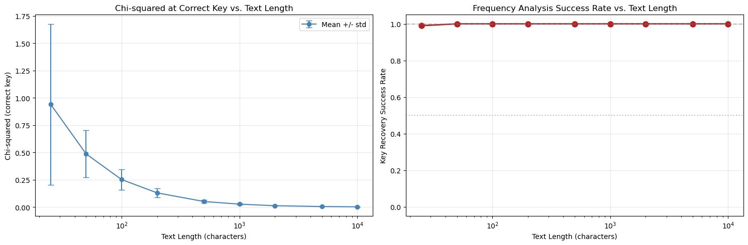
Experiment 3: Text Length and Frequency Analysis#
Reliability
How much ciphertext do we need for frequency analysis to work? We investigate by encrypting texts of varying length and measuring how well the chi-squared test recovers the correct key.
Show code cell source
import numpy as np
import matplotlib.pyplot as plt
%matplotlib inline
import string
import re

ENGLISH_FREQ = np.array([
    0.0817, 0.0129, 0.0278, 0.0425, 0.1270, 0.0223,
    0.0202, 0.0609, 0.0697, 0.0015, 0.0077, 0.0403,
    0.0241, 0.0675, 0.0751, 0.0193, 0.0010, 0.0599,
    0.0633, 0.0906, 0.0276, 0.0098, 0.0236, 0.0015,
    0.0197, 0.0007
])
ENGLISH_LETTERS = list(string.ascii_lowercase)

def clean_text(text):
    return re.sub(r'[^a-z]', '', text.lower())

def compute_frequency(text):
    cleaned = clean_text(text)
    if len(cleaned) == 0:
        return np.zeros(26)
    counts = np.array([cleaned.count(c) for c in ENGLISH_LETTERS])
    return counts / len(cleaned)

def chi_squared(observed, expected):
    mask = expected > 0
    return np.sum((observed[mask] - expected[mask])**2 / expected[mask])

def shift_encrypt(text, key):
    cleaned = clean_text(text)
    return ''.join(chr((ord(ch) - ord('a') + key) % 26 + ord('a')) for ch in cleaned)

# Generate a long pseudo-English text by sampling letters from the English distribution
np.random.seed(42)
# Normalize frequencies to sum exactly to 1.0 (required by np.random.choice)
english_prob = ENGLISH_FREQ / ENGLISH_FREQ.sum()
long_english = ''.join(np.random.choice(ENGLISH_LETTERS, size=20000, p=english_prob))

# Test parameters
lengths = [25, 50, 100, 200, 500, 1000, 2000, 5000, 10000]
KEY = 13
n_trials = 100  # Number of random trials per length

# For each length, run multiple trials and compute:
# 1. Chi-squared of the correct key
# 2. Fraction of trials where the correct key is recovered
chi2_means = []
chi2_stds = []
success_rates = []

for length in lengths:
    chi2_values = []
    successes = 0
    for trial in range(n_trials):
        # Draw a random substring of the given length
        start = np.random.randint(0, len(long_english) - length)
        snippet = long_english[start:start + length]

        # Encrypt
        cipher = shift_encrypt(snippet, KEY)
        cipher_freq = compute_frequency(cipher)

        # Try all shifts
        scores = np.array([chi_squared(np.roll(cipher_freq, -s), ENGLISH_FREQ) for s in range(26)])
        recovered = np.argmin(scores)

        chi2_values.append(scores[KEY])
        if recovered == KEY:
            successes += 1

    chi2_means.append(np.mean(chi2_values))
    chi2_stds.append(np.std(chi2_values))
    success_rates.append(successes / n_trials)

# Plot results
fig, axes = plt.subplots(1, 2, figsize=(15, 5))

# Left: chi-squared at correct key vs. text length
axes[0].errorbar(lengths, chi2_means, yerr=chi2_stds, fmt='o-', color='steelblue',
                 capsize=4, label='Mean +/- std')
axes[0].set_xscale('log')
axes[0].set_xlabel('Text Length (characters)')
axes[0].set_ylabel('Chi-squared (correct key)')
axes[0].set_title('Chi-squared at Correct Key vs. Text Length')
axes[0].legend()
axes[0].grid(True, alpha=0.3)

# Right: success rate vs. text length
axes[1].plot(lengths, success_rates, 'o-', color='firebrick', linewidth=2, markersize=8)
axes[1].set_xscale('log')
axes[1].set_xlabel('Text Length (characters)')
axes[1].set_ylabel('Key Recovery Success Rate')
axes[1].set_title('Frequency Analysis Success Rate vs. Text Length')
axes[1].set_ylim(-0.05, 1.05)
axes[1].axhline(y=1.0, color='gray', linestyle='--', alpha=0.5)
axes[1].axhline(y=0.5, color='gray', linestyle=':', alpha=0.5)
axes[1].grid(True, alpha=0.3)

plt.tight_layout()
plt.savefig('fig_ch03_exp3_length_vs_success.png', dpi=150, bbox_inches='tight')
plt.show()

# Print table
print(f'{"Length":>8s}  {"Mean chi2":>10s}  {"Std chi2":>10s}  {"Success Rate":>13s}')
print('-' * 48)
for i, length in enumerate(lengths):
    print(f'{int(length):8d}  {float(chi2_means[i]):10.6f}  {float(chi2_stds[i]):10.6f}  {float(success_rates[i]):13.2%}')
  Length   Mean chi2    Std chi2   Success Rate
------------------------------------------------
      25    0.940965    0.736695         99.00%
      50    0.486846    0.216307        100.00%
     100    0.251605    0.093468        100.00%
     200    0.130152    0.041346        100.00%
     500    0.050743    0.013690        100.00%
    1000    0.026730    0.007044        100.00%
    2000    0.012479    0.003084        100.00%
    5000    0.004832    0.001180        100.00%
   10000    0.002310    0.000407        100.00%
A Complete Shift Cipher#
Breaker
We now assemble all the pieces into a single function that, given an arbitrary ciphertext encrypted with a shift cipher, recovers the key and decrypts the message.
import numpy as np
import matplotlib.pyplot as plt
%matplotlib inline
import string
import re

ENGLISH_FREQ = np.array([
    0.0817, 0.0129, 0.0278, 0.0425, 0.1270, 0.0223,
    0.0202, 0.0609, 0.0697, 0.0015, 0.0077, 0.0403,
    0.0241, 0.0675, 0.0751, 0.0193, 0.0010, 0.0599,
    0.0633, 0.0906, 0.0276, 0.0098, 0.0236, 0.0015,
    0.0197, 0.0007
])
ENGLISH_LETTERS = list(string.ascii_lowercase)

def clean_text(text):
    return re.sub(r'[^a-z]', '', text.lower())

def compute_frequency(text):
    cleaned = clean_text(text)
    if len(cleaned) == 0:
        return np.zeros(26)
    counts = np.array([cleaned.count(c) for c in ENGLISH_LETTERS])
    return counts / len(cleaned)

def chi_squared(observed, expected):
    mask = expected > 0
    return np.sum((observed[mask] - expected[mask])**2 / expected[mask])

def shift_encrypt(text, key):
    cleaned = clean_text(text)
    return ''.join(chr((ord(ch) - ord('a') + key) % 26 + ord('a')) for ch in cleaned)

def shift_decrypt(text, key):
    return shift_encrypt(text, -key)


def break_shift_cipher(ciphertext, expected_freq=None, verbose=True):
    """
    Break a shift cipher by frequency analysis.

    Parameters
    ----------
    ciphertext : str
        The encrypted message (any casing/punctuation will be stripped).
    expected_freq : np.ndarray or None
        Expected letter frequency distribution. Defaults to English.
    verbose : bool
        If True, print detailed results.

    Returns
    -------
    dict
        Dictionary with keys: 'key', 'plaintext', 'chi2_scores', 'all_decryptions'.
    """
    if expected_freq is None:
        expected_freq = ENGLISH_FREQ

    cleaned = clean_text(ciphertext)
    cipher_freq = compute_frequency(cleaned)

    # Test all 26 candidate keys
    chi2_scores = np.zeros(26)
    decryptions = []
    for s in range(26):
        shifted_freq = np.roll(cipher_freq, -s)
        chi2_scores[s] = chi_squared(shifted_freq, expected_freq)
        decryptions.append(shift_decrypt(cleaned, s))

    best_key = int(np.argmin(chi2_scores))
    best_plaintext = decryptions[best_key]

    if verbose:
        print(f'Ciphertext length: {len(cleaned)} characters')
        print(f'Recovered key: k = {best_key}')
        print(f'Chi-squared at best key: {float(chi2_scores[best_key]):.6f}')
        print(f'\nDecrypted text (first 200 chars):')
        print(f'  {best_plaintext[:200]}')
        print()
        # Show top 3 candidates
        ranked = np.argsort(chi2_scores)
        print('Top 3 candidate keys:')
        for rank, k in enumerate(ranked[:3]):
            print(f'  #{rank+1}: k={int(k):2d}, chi2={float(chi2_scores[k]):.6f}, text={decryptions[k][:60]}...')

    return {
        'key': best_key,
        'plaintext': best_plaintext,
        'chi2_scores': chi2_scores,
        'all_decryptions': decryptions
    }


# ---- Demonstration ----
# Encrypt a message with an unknown key
secret_message = '''
The art of war teaches us to rely not on the likelihood of the enemy not coming
but on our own readiness to receive him not on the chance of his not attacking
but rather on the fact that we have made our position unassailable
'''

SECRET_KEY = 19
encrypted = shift_encrypt(secret_message, SECRET_KEY)
print('=' * 70)
print('SHIFT CIPHER BREAKER -- DEMONSTRATION')
print('=' * 70)
print(f'\nEncrypted message:')
print(f'  {encrypted[:100]}...')
print()

result = break_shift_cipher(encrypted)

# Verify
print(f'\nVerification: true key was k={SECRET_KEY}, recovered k={result["key"]}')
print(f'Correct: {result["key"] == SECRET_KEY}')
======================================================================
SHIFT CIPHER BREAKER -- DEMONSTRATION
======================================================================

Encrypted message:
  maxtkmhyptkmxtvaxlnlmhkxerghmhgmaxebdxebahhwhymaxxgxfrghmvhfbgzunmhghnkhpgkxtwbgxllmhkxvxboxabfghmhg...

Ciphertext length: 181 characters
Recovered key: k = 19
Chi-squared at best key: 0.102754

Decrypted text (first 200 chars):
  theartofwarteachesustorelynotonthelikelihoodoftheenemynotcomingbutonourownreadinesstoreceivehimnotonthechanceofhisnotattackingbutratheronthefactthatwehavemadeourpositionunassailable

Top 3 candidate keys:
  #1: k=19, chi2=0.102754, text=theartofwarteachesustorelynotonthelikelihoodoftheenemynotcom...
  #2: k=25, chi2=2.563491, text=nbyulnizqulnyuwbymomnilyfshinihnbyfceyfcbiixiznbyyhygshinwig...
  #3: k= 6, chi2=3.277783, text=gurnegbsjnegrnpurfhfgberylabgbaguryvxryvubbqbsgurrarzlabgpbz...

Verification: true key was k=19, recovered k=19
Correct: True
Show code cell source
import numpy as np
import matplotlib.pyplot as plt
%matplotlib inline
import string
import re

ENGLISH_FREQ = np.array([
    0.0817, 0.0129, 0.0278, 0.0425, 0.1270, 0.0223,
    0.0202, 0.0609, 0.0697, 0.0015, 0.0077, 0.0403,
    0.0241, 0.0675, 0.0751, 0.0193, 0.0010, 0.0599,
    0.0633, 0.0906, 0.0276, 0.0098, 0.0236, 0.0015,
    0.0197, 0.0007
])
ENGLISH_LETTERS = list(string.ascii_lowercase)

def clean_text(text):
    return re.sub(r'[^a-z]', '', text.lower())

def compute_frequency(text):
    cleaned = clean_text(text)
    if len(cleaned) == 0:
        return np.zeros(26)
    counts = np.array([cleaned.count(c) for c in ENGLISH_LETTERS])
    return counts / len(cleaned)

def shift_encrypt(text, key):
    cleaned = clean_text(text)
    return ''.join(chr((ord(ch) - ord('a') + key) % 26 + ord('a')) for ch in cleaned)

def shift_decrypt(text, key):
    return shift_encrypt(text, -key)

def chi_squared(observed, expected):
    mask = expected > 0
    return np.sum((observed[mask] - expected[mask])**2 / expected[mask])

# Use a different message for a second demonstration
mystery_text = '''
In the beginning God created the heaven and the earth And the earth was without form
and void and darkness was upon the face of the deep And the Spirit of God moved upon
the face of the waters And God said Let there be light and there was light And God saw
the light that it was good and God divided the light from the darkness And God called
the light Day and the darkness he called Night And the evening and the morning were
the first day
'''

KEY2 = 11
cipher2 = shift_encrypt(mystery_text, KEY2)
cipher2_freq = compute_frequency(cipher2)

# Compute chi-squared for all shifts
chi2_all = np.array([chi_squared(np.roll(cipher2_freq, -s), ENGLISH_FREQ) for s in range(26)])
best = int(np.argmin(chi2_all))

# Visualize: three panels
fig, axes = plt.subplots(1, 3, figsize=(18, 5))
x = np.arange(26)

# Panel 1: Ciphertext frequency
axes[0].bar(x, cipher2_freq, color='darkorange', alpha=0.8)
axes[0].scatter(x, ENGLISH_FREQ, color='red', s=25, zorder=5)
axes[0].set_xticks(x)
axes[0].set_xticklabels(ENGLISH_LETTERS, fontsize=8)
axes[0].set_title('Ciphertext Frequencies')
axes[0].set_ylabel('Relative Frequency')
axes[0].set_xlim(-0.6, 25.4)

# Panel 2: After applying the recovered shift
recovered_freq = np.roll(cipher2_freq, -best)
axes[1].bar(x, recovered_freq, color='seagreen', alpha=0.8)
axes[1].scatter(x, ENGLISH_FREQ, color='red', s=25, zorder=5, label='Expected English')
axes[1].set_xticks(x)
axes[1].set_xticklabels(ENGLISH_LETTERS, fontsize=8)
axes[1].set_title(f'After Shifting Back by k={best}')
axes[1].set_ylabel('Relative Frequency')
axes[1].set_xlim(-0.6, 25.4)
axes[1].legend(fontsize=8)

# Panel 3: Chi-squared landscape
colors = ['firebrick' if s == best else 'steelblue' for s in range(26)]
axes[2].bar(range(26), chi2_all, color=colors, alpha=0.8)
axes[2].set_xlabel('Candidate Key')
axes[2].set_ylabel('Chi-squared')
axes[2].set_title('Chi-squared Landscape')
axes[2].set_xticks(range(26))

plt.tight_layout()
plt.savefig('fig_ch03_breaker_visualization.png', dpi=150, bbox_inches='tight')
plt.show()

# Print the decrypted text
decrypted = shift_decrypt(cipher2, best)
print(f'Recovered key: k = {best} (true key: {KEY2})')
print(f'Decrypted text: {decrypted[:200]}')
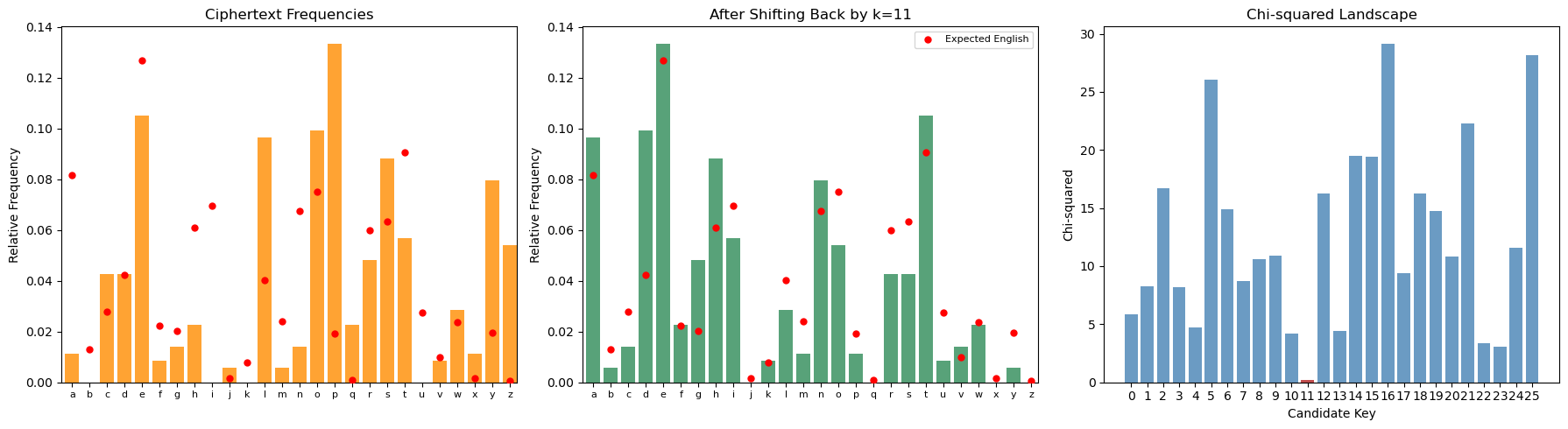
Recovered key: k = 11 (true key: 11)
Decrypted text: inthebeginninggodcreatedtheheavenandtheearthandtheearthwaswithoutformandvoidanddarknesswasuponthefaceofthedeepandthespiritofgodmoveduponthefaceofthewatersandgodsaidlettherebelightandtherewaslightandgo
3.4 Exercises#
3.5 Summary#
In this chapter we developed frequency analysis, the oldest and most fundamental technique in cryptanalysis.
Key concepts introduced:
Historical foundation. Al-Kindi’s ninth-century insight that natural languages have characteristic letter frequency distributions, and that these distributions are preserved (up to permutation) by monoalphabetic substitution ciphers.
Formal framework. We defined letter frequency, frequency distributions as vectors on the probability simplex, and two distance measures – Euclidean distance and the chi-squared statistic – for comparing observed and expected distributions.
Shift cipher cryptanalysis. We proved that a shift cipher cyclically permutes the frequency distribution, which means the key can be recovered by finding the shift that best aligns the ciphertext distribution with the expected English distribution. This requires testing only 26 candidates.
The role of text length. Frequency analysis is a statistical technique whose reliability depends on having sufficient data. Our experiments quantified this: with fewer than about 100 characters, the correct key is recovered only some of the time; with 500+ characters, success is nearly guaranteed.
Limitations. Frequency analysis works well against monoalphabetic ciphers but is defeated by polyalphabetic ciphers (Chapter 5), which flatten the frequency distribution by using multiple substitution alphabets. Understanding why frequency analysis fails against these more sophisticated ciphers motivates the cryptanalytic techniques developed in the coming chapters.
Looking ahead. In Chapter 4, we will examine the general monoalphabetic substitution cipher in more detail, exploring dictionary-based attacks and automated cryptanalysis. In Chapter 5, we encounter the Vigenere cipher, which was specifically designed to resist the frequency analysis attack developed here.
3.6 References#
Al-Kindi (c. 850 AD). Risalah fi Istikhraj al-Mu’amma (A Manuscript on Deciphering Cryptographic Messages). This is the earliest known treatise on cryptanalysis, introducing frequency analysis as a systematic technique for breaking monoalphabetic substitution ciphers. A translation and analysis can be found in: Al-Jubouri, I.M.N. (2004), History of Islamic Philosophy, and in the secondary literature cited below.
Singh, Simon (1999). The Code Book: The Science of Secrecy from Ancient Egypt to Quantum Cryptography. Doubleday. An outstanding popular account of the history of cryptography and cryptanalysis, with an excellent chapter on Al-Kindi and frequency analysis. Highly recommended for historical context and motivation.
Katz, Jonathan and Lindell, Yehuda (2020). Introduction to Modern Cryptography, 3rd edition. CRC Press. Chapter 1 provides a modern treatment of classical ciphers and their cryptanalysis, including shift and substitution ciphers. The formal definitions in this chapter follow their conventions.
Stinson, Douglas R. and Paterson, Maura B. (2019). Cryptography: Theory and Practice, 4th edition. CRC Press. Contains a rigorous treatment of frequency analysis, the chi-squared statistic applied to cryptanalysis, and the index of coincidence.
Lewand, Robert E. (2000). Cryptological Mathematics. Mathematical Association of America. Contains detailed tables of English letter, digram, and trigram frequencies, as well as frequency data for other languages. The frequency values used in this chapter are consistent with those reported in this reference.