
Chapter 16: Linear Cryptanalysis Foundations (SageMath)#
Python Version Available
This notebook contains the SageMath implementation. A pure Python/NumPy version is available in Chapter 16: Linear Cryptanalysis Foundations.
16.1 Historical Context: Matsui’s Breakthrough#
In 1993, at the EUROCRYPT conference in Lofthus, Norway, Mitsuru Matsui presented a paper that would fundamentally change the landscape of block cipher analysis. Titled “Linear Cryptanalysis Method for DES Cipher,” this work introduced a novel attack paradigm that exploited linear statistical relationships between plaintext bits, ciphertext bits, and key bits. Within a year, Matsui refined the method and demonstrated a practical key-recovery attack on the full 16-round Data Encryption Standard (DES) using approximately \(2^{43}\) known plaintext-ciphertext pairs – the first publicly known attack on full DES that was faster than brute-force search over the \(2^{56}\)-bit key space.
The significance of this achievement cannot be overstated. DES had been the de facto standard for symmetric encryption since 1977. Despite decades of intensive cryptanalytic scrutiny, no public attack had broken the full cipher faster than exhaustive key search. Differential cryptanalysis, introduced by Biham and Shamir in 1990, required \(2^{47}\) chosen plaintexts – a chosen-plaintext attack that was theoretically powerful but practically difficult to mount. Matsui’s linear cryptanalysis, by contrast, required only known plaintexts, making it significantly more practical in real-world scenarios where an attacker might passively collect plaintext-ciphertext pairs.
“The purpose of this paper is to present a new method, called linear cryptanalysis, for cryptanalysis of DES cipher and to show that DES is breakable with \(2^{43}\) known plaintext-ciphertext pairs.”
– Mitsuru Matsui, Linear Cryptanalysis Method for DES Cipher, EUROCRYPT 1993
The core idea behind linear cryptanalysis is deceptively simple. Consider a block cipher as a complex nonlinear function mapping plaintext \(P\) and key \(K\) to ciphertext \(C\). Although this function is designed to be highly nonlinear (to resist algebraic attacks), it is never perfectly nonlinear. For certain choices of bit positions – specified by input masks \(\alpha\) and output masks \(\beta\) – the XOR of selected plaintext bits and selected ciphertext bits correlates with the XOR of certain key bits:
This equation holds not with certainty, but with probability \(p = \frac{1}{2} + \varepsilon\), where \(\varepsilon\) is the bias. If \(\varepsilon\) is non-negligible, collecting enough known plaintext-ciphertext pairs allows the attacker to determine the value of the key-bit XOR with high confidence. By constructing multiple such linear approximations and combining them, the attacker can recover the full key.
Important
Linear cryptanalysis is a known-plaintext attack. Unlike differential cryptanalysis, which requires the attacker to choose specific plaintext pairs, linear cryptanalysis only requires the attacker to observe plaintext-ciphertext pairs encrypted under the same key. This makes it significantly more practical in many real-world scenarios.
Matsui’s work had profound consequences for cipher design. Every modern block cipher – including AES (Rijndael), Serpent, Twofish, and Camellia – is now explicitly designed to resist linear cryptanalysis. The maximum bias of the S-box linear approximation table became a primary design criterion, and the wide trail strategy used in AES was specifically engineered to ensure that any linear approximation spanning multiple rounds accumulates negligibly small bias.
16.2 Formal Definitions#
We now develop the mathematical foundations of linear cryptanalysis with full rigor. Throughout this section, we work over \(\mathbb{F}_2 = \{0, 1\}\), the field with two elements, where addition is XOR (\(\oplus\)).
Boolean Functions and Inner Products#
For a vector \(x = (x_1, x_2, \ldots, x_n) \in \mathbb{F}_2^n\) and a mask \(\alpha = (\alpha_1, \alpha_2, \ldots, \alpha_n) \in \mathbb{F}_2^n\), the inner product is:
This selects and XORs exactly those bits of \(x\) where the corresponding bit of \(\alpha\) is 1.
Definition 16.1 (Linear Approximation of a Boolean Function)
Let \(S: \mathbb{F}_2^n \to \mathbb{F}_2^m\) be a vectorial Boolean function (such as an S-box). A linear approximation of \(S\) with input mask \(\alpha \in \mathbb{F}_2^n\) and output mask \(\beta \in \mathbb{F}_2^m\) is the Boolean equation:
or equivalently:
The probability of this approximation is:
For a random function, we would expect \(p(\alpha, \beta) = 1/2\) for all non-trivial masks (i.e., \((\alpha, \beta) \neq (0, 0)\)). The degree to which an S-box deviates from this ideal is captured by the bias.
Definition 16.2 (Bias)
The bias of a linear approximation \((\alpha, \beta)\) for a function \(S\) is:
Equivalently, if we define the random variable \(X = \langle \alpha, x \rangle \oplus \langle \beta, S(x) \rangle\), then:
The bias satisfies \(-\frac{1}{2} \leq \varepsilon \leq \frac{1}{2}\), with \(\varepsilon = 0\) indicating a perfectly balanced (ideal) approximation.
Definition 16.3 (Linear Approximation Table)
The Linear Approximation Table (LAT) of an S-box \(S: \mathbb{F}_2^n \to \mathbb{F}_2^m\) is the \((2^n) \times (2^m)\) matrix \(\Lambda\) where:
Each entry \(\Lambda[\alpha][\beta]\) is related to the bias by \(\varepsilon(\alpha, \beta) = \Lambda[\alpha][\beta] / 2^n\).
The LAT has the following properties:
\(\Lambda[0][0] = 2^{n-1}\) (the trivial approximation always holds for all inputs, so the count is \(2^n\) and the entry is \(2^n - 2^{n-1} = 2^{n-1}\)).
\(\Lambda[\alpha][0] = 0\) for \(\alpha \neq 0\) (any non-trivial input mask with trivial output mask is balanced for a permutation).
All entries are integers with the same parity.
16.3 The Piling-Up Lemma#
The piling-up lemma is the theoretical engine that powers linear cryptanalysis. It tells us how to combine biases of individual round approximations to estimate the bias of a multi-round linear approximation.
Theorem 16.1 (Piling-Up Lemma, Matsui 1993)
Let \(X_1, X_2, \ldots, X_n\) be independent binary random variables with biases \(\varepsilon_i = \Pr[X_i = 0] - 1/2\) for \(i = 1, \ldots, n\). Then the bias of their XOR is:
That is, if \(Y = X_1 \oplus X_2 \oplus \cdots \oplus X_n\), then:
Proof of the Piling-Up Lemma
Base case (\(n = 2\)). Let \(X_1, X_2\) be independent binary random variables with \(\Pr[X_i = 0] = 1/2 + \varepsilon_i\), so \(\Pr[X_i = 1] = 1/2 - \varepsilon_i\).
We compute \(\Pr[X_1 \oplus X_2 = 0]\). Since \(X_1 \oplus X_2 = 0\) iff both are 0 or both are 1:
(by independence). Substituting:
Expanding and adding:
So the bias of \(X_1 \oplus X_2\) is \(2\varepsilon_1\varepsilon_2 = 2^{2-1}\varepsilon_1\varepsilon_2\). This confirms the formula for \(n = 2\).
Inductive step. Assume the result holds for \(n-1\) variables: the bias of \(Y_{n-1} = X_1 \oplus \cdots \oplus X_{n-1}\) is \(\varepsilon_{Y_{n-1}} = 2^{n-2}\prod_{i=1}^{n-1}\varepsilon_i\).
Now \(Y_n = Y_{n-1} \oplus X_n\). Since \(Y_{n-1}\) depends only on \(X_1, \ldots, X_{n-1}\) and \(X_n\) is independent of all of these, \(Y_{n-1}\) and \(X_n\) are independent. Applying the base case:
This completes the induction. \(\square\)
Warning
The independence assumption is crucial. The piling-up lemma assumes that the random variables \(X_1, \ldots, X_n\) are independent. In the context of a block cipher, these correspond to the linear approximations of individual S-boxes or individual rounds. In practice, the approximations are not perfectly independent because they share intermediate state bits. However, the heuristic assumption of independence (sometimes called the linear hull hypothesis) works remarkably well in practice, and the piling-up lemma gives good predictions for the bias of multi-round approximations.
16.4 The SPN Cryptosystem#
We analyze a simple cryptosystem described in the paper “A Tutorial on Linear and Differential Cryptanalysis” by Howard Heys.
Cryptosystem (basic Substitution-Permutation network)
Input: plaintext of 16 bits length
Output: ciphertext of 16 bits length
Key: 28-bit key which we split into four 16-bit round keys \(K_1, K_2, K_3, K_4\)
This cryptosystem consists of 3 rounds. In each round \(i\) we XOR with the round key \(K_i\), split a block of 16 bits into 4-bit subblocks to which we apply an S-box type transformation (non-linear). To each block we apply the same transformation. After that we apply to the list of 4 blocks a permutation \(P\). After the final round we XOR with the key \(K_4\).
# Permutation P
Plist = [0, 4, 8, 12, 1, 5, 9, 13, 2, 6, 10, 14, 3, 7, 11, 15]

G = SymmetricGroup(range(0, 16))
Pperm = PermutationGroupElement(Plist, G)

Pinvlist = [(Pperm**(-1))(i) for i in range(0, 16)]

def P(block16):
    return [block16[x] for x in Plist]

def Pinv(block16):
    return [block16[x] for x in Pinvlist]
# S-Box and helper functions

def BlockToHex(key):
    size = len(key) // 4
    hlist = []
    for i in range(0, size):
        kpart = key[4*i:4*i+4]
        hlist.append(hex(int(''.join(map(str, kpart)), base=2))[2:].upper())
    return ''.join(hlist)

def leftpadding(li, n):
    return [0]*(n - len(li)) + li

def HexToBlock(h):
    key = []
    for hel in h:
        key += leftpadding(list(map(int, bin(int(hel, base=16))[2:])), 4)
    return key

Sboxlist = ['E','4','D','1','2','F','B','8','3','A','6','C','5','9','0','7']

Sboxinvlist = ['E', '3', '4', '8', '1', 'C', 'A', 'F', '7', 'D', '9', '6', 'B', '2', '0', '5']

def SBox(chunk4):
    return HexToBlock(Sboxlist[int(BlockToHex(chunk4), base=16)])

def SBoxinv(chunk4):
    return HexToBlock(Sboxinvlist[int(BlockToHex(chunk4), base=16)])

def S(block16):
    Sout = []
    for i in range(0, 4):
        Sout += SBox(block16[4*i:4*(i+1)])
    return Sout

def Sinv(block16):
    Sout = []
    for i in range(0, 4):
        Sout += SBoxinv(block16[4*i:4*(i+1)])
    return Sout
SBox([0, 0, 0, 0])
[1, 1, 1, 0]
# XORing lists (using SageMath ^^ for XOR)
def ListXOR(li1, li2):
    return [li1[i]^^li2[i] for i in range(0, len(li1))]
# Key schedule
def KeySchedule(key28):
    return [key28[4*i:4*(i+4)] for i in range(0, 4)]

def RoundKey(expkey, r):
    return expkey[r]
def SPNEncryption(plaintext16, key28):
    expkey = KeySchedule(key28)
    state = plaintext16

    # round 1
    state = ListXOR(state, RoundKey(expkey, 0))
    state = S(state)
    state = P(state)

    # round 2
    state = ListXOR(state, RoundKey(expkey, 1))
    state = S(state)
    state = P(state)

    # round 3
    state = ListXOR(state, RoundKey(expkey, 2))
    state = S(state)

    # final XOR
    state = ListXOR(state, RoundKey(expkey, 3))

    return state
def SPNDecryption(plaintext16, key28):
    expkey = KeySchedule(key28)
    state = plaintext16

    state = ListXOR(state, RoundKey(expkey, 3))
    state = Sinv(state)
    state = ListXOR(state, RoundKey(expkey, 2))
    state = Pinv(state)
    state = Sinv(state)
    state = ListXOR(state, RoundKey(expkey, 1))
    state = Pinv(state)
    state = Sinv(state)
    state = ListXOR(state, RoundKey(expkey, 0))

    return state
# Verify encryption/decryption roundtrip
li = [choice([0, 1]) for _ in range(0, 16)]
k = [choice([0, 1]) for _ in range(0, 28)]
SPNDecryption(SPNEncryption(li, k), k) == li
True
16.5 Building the Bias Table (Linear Approximation Table)#
We build a bias table for the S-box. The bias \(\varepsilon(X)\) of a Boolean random variable \(X\) is defined by the formula \(P(X=0) - 1/2\). In particular, when \(P(X=0) = 1/2\) the bias is \(0\) (no useful information encoded in the variable \(X\)). When \(\varepsilon(X) = \pm 1/2\) we have a completely determined variable \(X\) (most useful case).
Independent random Boolean variables \(X_1, \ldots, X_n\) satisfy the Piling-Up Lemma:
We compute the full \(16 \times 16\) LAT using SageMath’s matrix() over ZZ, and display it as a matrix_plot().
def TestLinEq(X, Y, lin):
    a1, a2, a3, a4, b1, b2, b3, b4 = list(lin)
    X1, X2, X3, X4 = list(X)
    Y1, Y2, Y3, Y4 = list(Y)
    return (a1*X1 + a2*X2 + a3*X3 + a4*X4 + b1*Y1 + b2*Y2 + b3*Y3 + b4*Y4) % 2 == 0


flin = lambda X, coo: TestLinEq(X, SBox(X), coo)

def biascoo(coo):
    li = [[X1, X2, X3, X4] for X1 in [0, 1] for X2 in [0, 1]
          for X3 in [0, 1] for X4 in [0, 1] if flin([X1, X2, X3, X4], coo)]
    return li

biasf = lambda li: len(li)/16 - 1/2
bij = lambda i, j: biasf(biascoo(
    leftpadding((ZZ(i).digits(base=2))[::-1], 4) +
    leftpadding((ZZ(j).digits(base=2))[::-1], 4)))

# Full LAT as a SageMath matrix
LAT = matrix(16, 16, [[bij(i, j) for i in range(0, 16)] for j in range(0, 16)])
LAT
[ 1/2    0    0    0    0    0    0    0    0    0    0    0    0    0    0    0]
[   0    0    0    0  1/8 -1/8  1/8 -1/8    0    0  1/4  1/4 -1/8  1/8  1/8 -1/8]
[   0 -1/8 -1/8    0    0 -1/8 -1/8    0    0 -1/8 -1/8    0  1/4  1/8  1/8 -1/4]
[   0 -1/8 -1/8    0 -1/8    0  1/4  1/8    0 -1/8  1/8 -1/4 -1/8    0    0 -1/8]
[   0    0    0    0 -1/8 -1/8  1/8  1/8    0    0 -1/4  1/4 -1/8 -1/8 -1/8 -1/8]
[   0    0    0    0 -1/4    0    0 -1/4    0    0    0    0    0  1/4 -1/4    0]
[   0 -1/8 -1/8    0 -1/8  1/4    0  1/8    0 -1/8  1/8  1/4  1/8    0    0  1/8]
[   0  3/8 -1/8    0    0  1/8  1/8    0    0 -1/8 -1/8    0    0  1/8  1/8    0]
[   0  1/8    0  1/8    0 -1/8    0 -1/8 -1/8 -1/4  1/8    0  1/8 -1/4 -1/8    0]
[   0  1/8    0 -3/8 -1/8    0 -1/8    0  1/8    0  1/8    0    0 -1/8    0 -1/8]
[   0    0  1/8 -1/8    0 -1/4  1/8  1/8  1/8 -1/8    0    0  1/8  1/8    0  1/4]
[   0    0  1/8 -1/8  1/8  1/8  1/4    0 -1/8  1/8    0    0  1/4    0 -1/8 -1/8]
[   0  1/8    0  1/8  1/8    0 -1/8  1/4  1/8    0  1/8    0    0  1/8 -1/4 -1/8]
[   0  1/8    0  1/8 -1/4 -1/8    0  1/8 -1/8  1/4  1/8    0  1/8    0  1/8    0]
[   0    0 -3/8 -1/8  1/8 -1/8    0    0 -1/8  1/8    0    0    0    0 -1/8  1/8]
[   0    0  1/8 -1/8    0    0 -1/8  1/8 -3/8 -1/8    0    0 -1/8  1/8    0    0]
Visualizing the Linear Approximation Table#
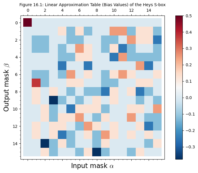
The LAT reveals the linear structure hidden within a nonlinear S-box. We use SageMath’s matrix_plot() to create a heatmap visualization that makes it easy to spot strong approximations.
# Visualize the LAT using SageMath's matrix_plot
# Convert to numerical matrix for plotting
LAT_numerical = matrix(RR, 16, 16, [[bij(i, j) for i in range(0, 16)] for j in range(0, 16)])
p = matrix_plot(LAT_numerical, cmap='RdBu_r', colorbar=True,
                axes_labels=['Input mask $\\alpha$', 'Output mask $\\beta$'])
p.show(title='Figure 16.1: Linear Approximation Table (Bias Values) of the Heys S-box',
       figsize=8)
Identifying the Strongest Approximations#
The most useful linear approximations for an attacker are those with the largest absolute bias. Let us extract and examine them.
# Find the top linear approximations with largest absolute bias
results = []
for alpha in range(16):
    for beta in range(16):
        if alpha == 0 and beta == 0:
            continue
        b = bij(alpha, beta)
        results.append((alpha, beta, b))

results.sort(key=lambda t: abs(t[2]), reverse=True)

print("Top 15 Linear Approximations for Heys S-box")
print("=" * 62)
print(f"{'Rank':>4s}  {'alpha':>6s}  {'beta':>6s}  {'Bias':>10s}  {'|Bias|':>8s}")
print("-" * 62)
for rank, (a, b, bias) in enumerate(results[:15], 1):
    alpha_bits = ''.join(str(x) for x in leftpadding((ZZ(a).digits(base=2))[::-1], 4))
    beta_bits = ''.join(str(x) for x in leftpadding((ZZ(b).digits(base=2))[::-1], 4))
    print(f"{int(rank):4d}  0x{a:01X} ({alpha_bits})  0x{b:01X} ({beta_bits})  {float(bias)):10.4f}  {float(abs(bias))):8.4f}")

print()
max_abs_bias = max(abs(r[2]) for r in results)
count_max = sum(1 for r in results if abs(r[2]) == max_abs_bias)
print(f"Maximum absolute bias: {float(max_abs_bias)):.4f}")
print(f"Number of approximations achieving max |bias|: {count_max}")
Top 15 Linear Approximations for Heys S-box
==============================================================
Rank   alpha    beta        Bias    |Bias|
--------------------------------------------------------------
   1  0x1 (0001)  0x7 (0111)      0.3750    0.3750
   2  0x2 (0010)  0xE (1110)     -0.3750    0.3750
   3  0x3 (0011)  0x9 (1001)     -0.3750    0.3750
   4  0x8 (1000)  0xF (1111)     -0.3750    0.3750
   5  0x4 (0100)  0x5 (0101)     -0.2500    0.2500
   6  0x4 (0100)  0xD (1101)     -0.2500    0.2500
   7  0x5 (0101)  0x6 (0110)      0.2500    0.2500
   8  0x5 (0101)  0xA (1010)     -0.2500    0.2500
   9  0x6 (0110)  0x3 (0011)      0.2500    0.2500
  10  0x6 (0110)  0xB (1011)      0.2500    0.2500
  11  0x7 (0111)  0x5 (0101)     -0.2500    0.2500
  12  0x7 (0111)  0xC (1100)      0.2500    0.2500
  13  0x9 (1001)  0x8 (1000)     -0.2500    0.2500
  14  0x9 (1001)  0xD (1101)      0.2500    0.2500
  15  0xA (1010)  0x1 (0001)      0.2500    0.2500

Maximum absolute bias: 0.3750
Number of approximations achieving max |bias|: 4
16.6 Experimental Verification of the Piling-Up Lemma#
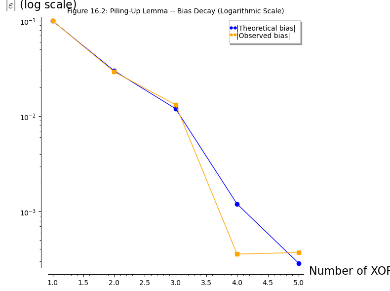
The piling-up lemma predicts how biases compose when independent random variables are XORed. Let us verify this experimentally by generating biased random variables and comparing the observed bias of their XOR against the theoretical prediction.
set_random_seed(42)

def generate_biased_bits(n_samples, bias):
    """
    Generate n_samples binary random variables with given bias.
    P(X=0) = 0.5 + bias, P(X=1) = 0.5 - bias
    """
    prob_zero = 0.5 + float(bias)
    return [0 if random() < prob_zero else 1 for _ in range(n_samples)]

def observed_bias(bits):
    """Compute observed bias: P(X=0) - 0.5"""
    return sum(1 for b in bits if b == 0) / len(bits) - 0.5

# Experiment: XOR of n biased variables
n_samples = 500000
individual_biases = [0.1, -0.15, 0.2, 0.05, -0.12]

print("Piling-Up Lemma Verification")
print("=" * 70)
print(f"Number of samples: {n_samples}")
print()

# Generate individual biased bits
bits_list = [generate_biased_bits(n_samples, eps) for eps in individual_biases]

# Verify individual biases
print("Individual variable biases:")
for i, (eps_true, bits) in enumerate(zip(individual_biases, bits_list)):
    eps_obs = observed_bias(bits)
    print(f"  X_{i+1}: true bias = {eps_true:+.4f}, observed bias = {eps_obs:+.4f}")
print()

# XOR progressively more variables and check
xor_bits = list(bits_list[0])
theoretical_biases = [individual_biases[0]]
observed_biases_list = [observed_bias(xor_bits)]
n_vars_list = [1]

print("Progressive XOR results:")
print(f"{'n vars':>7s}  {'Theoretical bias':>18s}  {'Observed bias':>16s}  {'Relative error':>16s}")
print("-" * 65)

theo = individual_biases[0]
obs = observed_bias(xor_bits)
rel_err = abs(theo - obs) / abs(theo) if theo != 0 else 0
print(f"{int(1):7d}  {float(theo):+18.8f}  {float(obs):+16.8f}  {float(rel_err)):16.4%}")

for k in range(1, len(individual_biases)):
    xor_bits = [xor_bits[i]^^bits_list[k][i] for i in range(n_samples)]

    # Piling-up lemma: bias = 2^{n-1} * product of individual biases
    n_combined = k + 1
    theo = (2**(n_combined - 1)) * prod(individual_biases[:n_combined])
    obs = observed_bias(xor_bits)
    rel_err = abs(theo - obs) / abs(theo) if theo != 0 else 0

    theoretical_biases.append(theo)
    observed_biases_list.append(obs)
    n_vars_list.append(n_combined)

    print(f"{int(n_combined):7d}  {float(theo):+18.8f}  {float(obs):+16.8f}  {float(rel_err)):16.4%}")
Piling-Up Lemma Verification
======================================================================
Number of samples: 500000
Individual variable biases:
  X_1: true bias = +0.1000, observed bias = +0.1002
  X_2: true bias = -0.1500, observed bias = -0.1489
  X_3: true bias = +0.2000, observed bias = +0.2001
  X_4: true bias = +0.0500, observed bias = +0.0499
  X_5: true bias = -0.1200, observed bias = -0.1189

Progressive XOR results:
 n vars    Theoretical bias     Observed bias    Relative error
-----------------------------------------------------------------
      1         +0.10000000       +0.10024400           0.2440%
      2         -0.03000000       -0.02931000           2.3000%
      3         -0.01200000       -0.01319600           9.9667%
      4         -0.00120000       -0.00035800          70.1667%
      5         +0.00028800       +0.00037200          29.1667%
# Visualize Piling-Up Lemma results using SageMath plotting
# Bar chart comparing theoretical vs observed biases
theo_data = [(i - 0.15, float(theoretical_biases[i])) for i in range(len(n_vars_list))]
obs_data = [(i + 0.15, float(observed_biases_list[i])) for i in range(len(n_vars_list))]

p1 = bar_chart([float(t) for t in theoretical_biases], color='blue', width=0.35)
p2 = bar_chart([float(o) for o in observed_biases_list], color='orange', width=0.35)

# Use list_plot for log-scale comparison of |bias|
abs_theo = [(n_vars_list[i], float(abs(theoretical_biases[i]))) for i in range(len(n_vars_list))]
abs_obs = [(n_vars_list[i], float(abs(observed_biases_list[i]))) for i in range(len(n_vars_list))]

p = list_plot(abs_theo, plotjoined=True, marker='o', color='blue',
              legend_label='|Theoretical bias|', scale='semilogy') + \
    list_plot(abs_obs, plotjoined=True, marker='s', color='orange',
              legend_label='|Observed bias|', scale='semilogy')
p.axes_labels(['Number of XORed Variables', '$|\\varepsilon|$ (log scale)'])
p.show(title='Figure 16.2: Piling-Up Lemma -- Bias Decay (Logarithmic Scale)', figsize=8)
16.7 Comparing S-box Linearity: Heys vs PRESENT vs Random#
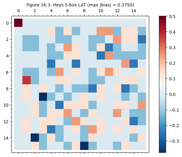
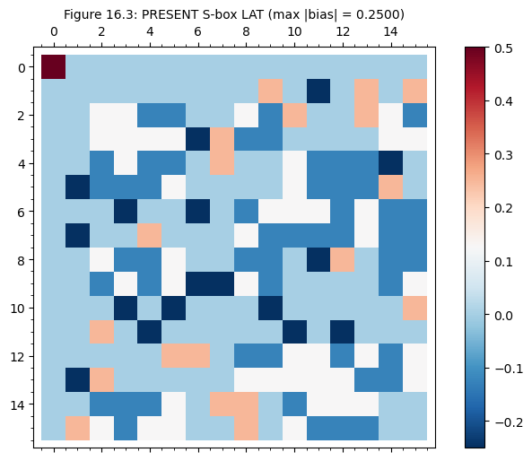
A well-designed S-box should minimize the maximum absolute bias in its LAT (excluding the trivial entry). Let us compare three S-boxes:
Heys S-box – the 4-bit educational S-box from Heys’ tutorial
PRESENT S-box – a well-designed 4-bit S-box from the PRESENT lightweight cipher, which is known to achieve optimal nonlinearity
Random permutation – a randomly generated 4-bit permutation
For an ideal \(n\)-bit S-box, the maximum absolute bias is bounded below by \(2^{-n/2}\) (the “bent function” bound for \(n\) even). For \(n = 4\), this gives \(|\varepsilon|_{\max} \geq 1/4\), so no 4-bit S-box can achieve maximum bias below \(1/4\).
def compute_lat_sbox(sbox_list):
    """Compute LAT for an S-box given as a list of hex values."""
    def sbox_apply(chunk4, sbox):
        return HexToBlock(sbox[int(BlockToHex(chunk4), base=16)])

    def test_lin(X, coo, sbox):
        a1, a2, a3, a4, b1, b2, b3, b4 = list(coo)
        X1, X2, X3, X4 = list(X)
        Y = sbox_apply(X, sbox)
        Y1, Y2, Y3, Y4 = list(Y)
        return (a1*X1 + a2*X2 + a3*X3 + a4*X4 + b1*Y1 + b2*Y2 + b3*Y3 + b4*Y4) % 2 == 0

    def bias_coo(coo, sbox):
        li = [[X1, X2, X3, X4] for X1 in [0, 1] for X2 in [0, 1]
              for X3 in [0, 1] for X4 in [0, 1] if test_lin([X1, X2, X3, X4], coo, sbox)]
        return len(li)/16 - 1/2

    M = matrix(RR, 16, 16)
    for i in range(16):
        for j in range(16):
            coo = leftpadding((ZZ(i).digits(base=2))[::-1], 4) + \
                  leftpadding((ZZ(j).digits(base=2))[::-1], 4)
            M[j, i] = bias_coo(coo, sbox_list)
    return M

# Define the three S-boxes
HEYS_SBOX_LIST = ['E','4','D','1','2','F','B','8','3','A','6','C','5','9','0','7']
PRESENT_SBOX_LIST = ['C','5','6','B','9','0','A','D','3','E','F','8','4','7','1','2']

set_random_seed(2023)
RANDOM_PERM = Permutations(16).random_element()
RANDOM_SBOX_LIST = [hex(x - 1)[2:].upper() for x in RANDOM_PERM]

sboxes = {'Heys': HEYS_SBOX_LIST, 'PRESENT': PRESENT_SBOX_LIST, 'Random': RANDOM_SBOX_LIST}

# Compute and display LATs
lats = {}
for name, sbox in sboxes.items():
    lats[name] = compute_lat_sbox(sbox)
    # Max absolute bias (excluding trivial (0,0) entry)
    max_bias = max(abs(lats[name][i, j]) for i in range(16) for j in range(16)
                   if not (i == 0 and j == 0))
    print(f"{name:10s} S-box: max |bias| = {float(max_bias)):.4f}  (ideal >= 0.2500)")
Heys       S-box: max |bias| = 0.3750  (ideal >= 0.2500)
PRESENT    S-box: max |bias| = 0.2500  (ideal >= 0.2500)
Random     S-box: max |bias| = 0.3750  (ideal >= 0.2500)
# Visualize all three LATs using SageMath matrix_plot
plots = []
for name in ['Heys', 'PRESENT', 'Random']:
    p = matrix_plot(lats[name], cmap='RdBu_r', colorbar=True)
    p.axes_labels(['$\\alpha$', '$\\beta$'])
    plots.append(p)

# Show them individually (SageMath does not have subplot in the same way)
for name in ['Heys', 'PRESENT', 'Random']:
    p = matrix_plot(lats[name], cmap='RdBu_r', colorbar=True)
    max_b = max(abs(lats[name][i, j]) for i in range(16) for j in range(16)
               if not (i == 0 and j == 0))
    p.show(title=f'Figure 16.3: {name} S-box LAT (max |bias| = {float(max_b)):.4f})',
           figsize=7)

16.8 Nonlinearity and the Walsh-Hadamard Transform#
The LAT is intimately related to the Walsh-Hadamard transform, which provides an efficient way to compute all entries simultaneously. The nonlinearity of an S-box – a key design metric – is defined in terms of the maximum absolute value in the LAT.
Definition 16.4 (Nonlinearity of an S-box)
The nonlinearity of an S-box \(S: \mathbb{F}_2^n \to \mathbb{F}_2^n\) is:
Higher nonlinearity means better resistance to linear cryptanalysis. For a 4-bit S-box (\(n = 4\)), the maximum achievable nonlinearity is \(2^{n-1} - 2^{n/2-1} = 8 - 2 = 4\) (in the LAT-count metric, this means \(\max |\Lambda| = 4\)).
Let us compute the nonlinearity of our three S-boxes using SageMath.
# Nonlinearity analysis
print("Nonlinearity Analysis")
print("=" * 60)
print()
nonlinearities = {}
max_biases_dict = {}
for name, sbox in sboxes.items():
lat_m = lats[name]
n = 16 # 2^4
# Max absolute LAT entry (excluding (0,0))
# LAT entries are bias values; convert to counts: count = bias * 16
max_lat_bias = max(abs(lat_m[i, j]) for i in range(n) for j in range(n)
if not (i == 0 and j == 0))
max_lat_count = int(max_lat_bias * n) # convert bias to count
nonlinearity = (n // 2) - max_lat_count
nonlinearities[name] = nonlinearity
max_biases_dict[name] = float(max_lat_bias)
print(f" {name:10s} S-box:")
print(f" Max |LAT count entry| = {max_lat_count}")
print(f" Nonlinearity NL(S) = {n//2} - {max_lat_count} = {nonlinearity}")
print(f" Max |bias| = {float(max_lat_bias)):.4f}")
print()
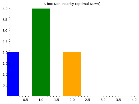
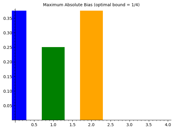
# Visualization using SageMath bar_chart
names = list(sboxes.keys())
nl_values = [nonlinearities[n] for n in names]
mb_values = [max_biases_dict[n] for n in names]
p1 = bar_chart(nl_values, color=['blue', 'green', 'orange'], width=0.6)
p1.show(title='S-box Nonlinearity (optimal NL=4)', figsize=6)
p2 = bar_chart(mb_values, color=['blue', 'green', 'orange'], width=0.6)
p2.show(title='Maximum Absolute Bias (optimal bound = 1/4)', figsize=6)
Nonlinearity Analysis
============================================================

  Heys       S-box:
    Max |LAT count entry| = 6
    Nonlinearity NL(S)   = 8 - 6 = 2
    Max |bias|           = 0.3750

  PRESENT    S-box:
    Max |LAT count entry| = 4
    Nonlinearity NL(S)   = 8 - 4 = 4
    Max |bias|           = 0.2500

  Random     S-box:
    Max |LAT count entry| = 6
    Nonlinearity NL(S)   = 8 - 6 = 2
    Max |bias|           = 0.3750
16.9 Statistical Properties of the LAT: Parseval’s Relation#
The entries of the LAT are not arbitrary integers – they obey specific structural constraints.
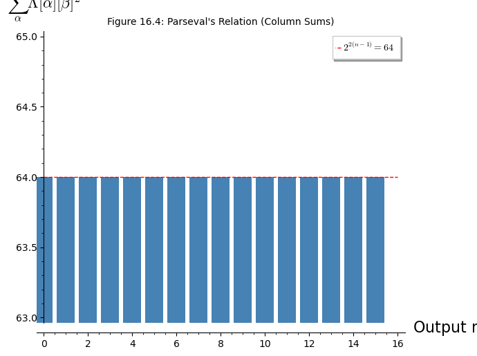
Theorem 16.3 (Parseval’s Relation for the LAT)
For any S-box \(S: \mathbb{F}_2^n \to \mathbb{F}_2^n\) (a permutation), and for any fixed output mask \(\beta \neq 0\):
This is the Parseval relation, and it implies that the “energy” in each column of the LAT is fixed. If one entry is large, others must be correspondingly smaller.
Let us verify Parseval’s relation numerically.
# Parseval's Relation Verification using the Heys S-box LAT
# Convert bias table to LAT counts: LAT_count[alpha][beta] = bias * 16
LAT_counts = matrix(ZZ, 16, 16, [[int(LAT[i][j] * 16) for j in range(16)] for i in range(16)])

print("Parseval's Relation Verification for the Heys S-box")
print("=" * 55)
print()
print(f"Expected: sum_alpha LAT[alpha][beta]^2 = 2^{{2(n-1)}} = 2^6 = {2^6}")
print()

print(f"{'beta':>6s}  {'Sum of squares':>16s}  {'Expected':>10s}  {'Match':>6s}")
print("-" * 46)

all_match = True
for beta in range(1, 16):
    col_sum_sq = sum(LAT_counts[alpha, beta]^2 for alpha in range(16))
    expected = 2^6  # = 64
    match = (col_sum_sq == expected)
    if not match:
        all_match = False
    print(f"0x{beta:01X}     {int(col_sum_sq):16d}  {int(expected):10d}  {'Yes' if match else 'NO':>6s}")

print()
print(f"All columns satisfy Parseval's relation: {all_match}")
print()

# Row-wise check
print("Row-wise check (fixed alpha, sum over beta):")
print(f"{'alpha':>6s}  {'Sum of squares':>16s}")
print("-" * 28)
for alpha in range(1, 16):
    row_sum_sq = sum(LAT_counts[alpha, beta]^2 for beta in range(16))
    print(f"0x{alpha:01X}     {int(row_sum_sq):16d}")

print()
print("Note: Row sums also equal 64 = 2^6 for this permutation S-box.")
print("This is because Parseval's relation holds both row-wise and column-wise")
print("for bijective S-boxes.")
Parseval's Relation Verification for the Heys S-box
=======================================================

Expected: sum_alpha LAT[alpha][beta]^2 = 2^{2(n-1)} = 2^6 = 64

  beta    Sum of squares    Expected   Match
----------------------------------------------
0x1                   64          64     Yes
0x2                   64          64     Yes
0x3                   64          64     Yes
0x4                   64          64     Yes
0x5                   64          64     Yes
0x6                   64          64     Yes
0x7                   64          64     Yes
0x8                   64          64     Yes
0x9                   64          64     Yes
0xA                   64          64     Yes
0xB                   64          64     Yes
0xC                   64          64     Yes
0xD                   64          64     Yes
0xE                   64          64     Yes
0xF                   64          64     Yes

All columns satisfy Parseval's relation: True

Row-wise check (fixed alpha, sum over beta):
 alpha    Sum of squares
----------------------------
0x1                   64
0x2                   64
0x3                   64
0x4                   64
0x5                   64
0x6                   64
0x7                   64
0x8                   64
0x9                   64
0xA                   64
0xB                   64
0xC                   64
0xD                   64
0xE                   64
0xF                   64

Note: Row sums also equal 64 = 2^6 for this permutation S-box.
This is because Parseval's relation holds both row-wise and column-wise
for bijective S-boxes.
# Visualize energy distribution across columns
col_energies = [sum(LAT_counts[alpha, beta]^2 for alpha in range(16))
for beta in range(16)]
p = bar_chart(col_energies, color='steelblue', width=0.8)
p += line([(0, 64), (16, 64)], color='red', linestyle='--', legend_label='$2^{2(n-1)} = 64$')
p.axes_labels(['Output mask $\\beta$', '$\\sum_{\\alpha} \\Lambda[\\alpha][\\beta]^2$'])
p.show(title="Figure 16.4: Parseval's Relation (Column Sums)", figsize=7)
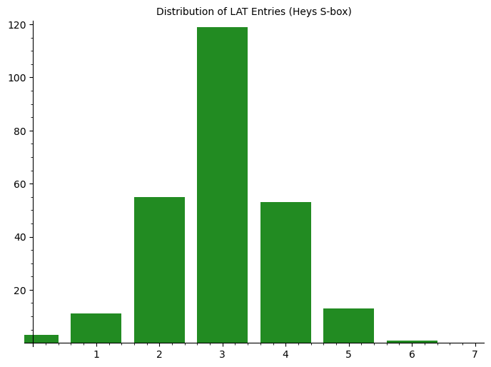
# Distribution of LAT entries
all_entries = [int(LAT_counts[a, b]) for a in range(16) for b in range(16)
if not (a == 0 and b == 0)]
unique_vals = sorted(set(all_entries))
counts = [all_entries.count(v) for v in unique_vals]
p2 = bar_chart(counts, color='forestgreen', width=0.8)
p2.show(title='Distribution of LAT Entries (Heys S-box)', figsize=7)
16.10 Data Complexity of Linear Cryptanalysis#
A crucial question for the practitioner is: how many known plaintexts are needed to exploit a linear approximation with bias \(\varepsilon\)?
Theorem 16.2 (Data Complexity)
To distinguish a linear approximation with bias \(\varepsilon\) from a random guess (bias 0) with success probability \(\geq 97.7\%\), the number of known plaintext-ciphertext pairs required is approximately:
More precisely, using a sign-determination test, the success probability after \(N\) samples is:
where \(\Phi\) is the standard normal CDF. Setting \(P_{\text{success}} = 0.977\) (corresponding to \(2\sigma\)) gives \(N \approx 1/\varepsilon^2\).
This inverse-square relationship means that halving the bias requires four times as many plaintexts.
# Matsui estimate for the required number of plaintext-ciphertext pairs
# Using the Piling-Up Lemma bias from our SPN
ee = (1/4)^3 * 4  # Matsui estimate constant/epsilon^2
print(f"Piling-up lemma combined bias epsilon = {float(ee)):.6f}")
print(f"Required number of plaintext-ciphertext pairs (8/epsilon^2): {float(8/ee^2)):.0f}")
print(f"Finding remaining digits requires checking about 2^20 = {2^20} keys")
Piling-up lemma combined bias epsilon = 0.062500
Required number of plaintext-ciphertext pairs (8/epsilon^2): 2048
Finding remaining digits requires checking about 2^20 = 1048576 keys
16.11 Mounting a Linear Analysis#
Attack (S-box Approximation)
We use the bias table above to mount an attack via Matsui’s linear cryptanalysis. This will require about 3000 pairs of plaintext-ciphertext to work and improve by a factor of 256 over brute force attack (shorten the attack from about 2 days to around 5 minutes).
We first use SageMath’s PolynomialRing over GF(2) to express the linear relations symbolically.
R.<X0,X1,X2,X3,Y0,Y1,Y2,Y3> = PolynomialRing(GF(2), 8)
# First linear relation: X3 + Y1 + Y2 + Y3
print("Relation 1:", X3 + Y1 + Y2 + Y3)
print("Bias:", biasf(biascoo([0, 0, 0, 1, 0, 1, 1, 1])))
Relation 1: X3 + Y1 + Y2 + Y3
Bias: 3/8
# Second linear relation: X2 + Y0 + Y1 + Y2
print("Relation 2:", X2 + Y0 + Y1 + Y2)
print("Bias:", biasf(biascoo([0, 0, 1, 0, 1, 1, 1, 0])))
Relation 2: X2 + Y0 + Y1 + Y2
Bias: -3/8
# We use the following two key relations
# Relation: X0 + X2 + X3 + Y1
print("Relation (used): X0 + X2 + X3 + Y1")
print("Bias:", biasf(biascoo([1, 0, 1, 1, 0, 1, 0, 0])))
Relation (used): X0 + X2 + X3 + Y1
Bias: 1/4
# Relation: X1 + Y1 + Y3
print("Relation (used): X1 + Y1 + Y3")
print("Bias:", biasf(biascoo([0, 1, 0, 0, 0, 1, 0, 1])))
Relation (used): X1 + Y1 + Y3
Bias: -1/4
Round Variable Notation#
We use the following notation:
\(U_{r,i}\) – \(i\)-th bit of the \(r\)-th round S-box input
\(V_{r,i}\) – \(i\)-th bit of the \(r\)-th round S-box output
\(K_{r,i}\) – \(i\)-th bit of the \(r\)-th round key
\(P_i\) – \(i\)-th bit of the plaintext
From the two equations above we deduce three relations:
R1: \(U_{0,4} + U_{0,6} + U_{0,7} + V_{0,5}\)
R2: \(U_{1,5} + V_{1,5} + V_{1,7}\)
R3: \(U_{2,5} + V_{2,5} + V_{2,7}\)
R4: \(U_{2,13} + V_{2,13} + V_{2,15}\)
Apply the Piling-Up Lemma (assuming independence) to chain these across rounds.
# Check permutation indices used in the chain
print("P(5) =", Plist[5])
print("P(7) =", Plist[7])
P(5) = 5
P(7) = 13
Combined Linear Equation Across Rounds#
Combining through the permutation layer, we get:
The key bits involved are:
# Key bits involved in the linear approximation
ks = KeySchedule([i for i in range(0, 28)])
print("Key bit indices: [K0_4, K0_6, K0_7, K1_5, K2_5, K2_13]")
print([ks[0][4], ks[0][6], ks[0][7], ks[1][5], ks[2][5], ks[2][13]])
Key bit indices: [K0_4, K0_6, K0_7, K1_5, K2_5, K2_13]
[4, 6, 7, 9, 13, 21]
Running the Linear Cryptanalysis Attack#
We generate 3000 plaintext-ciphertext pairs and use the linear approximation to recover 8 bits of the last round key.
# Generate plaintext-ciphertext pairs
secret_key = sum([leftpadding((ZZ(a).digits(base=2))[::-1], 4)
                  for a in [13, 5, 3, 6, 10, 11, 8]], [])

pcpairs = []
for _ in range(0, 3000):
    pli = [choice([0, 1]) for _ in range(0, 16)]
    cli = SPNEncryption(pli, secret_key)
    pcpairs.append([pli, cli])

print(f"Generated {len(pcpairs)} plaintext-ciphertext pairs")
Generated 3000 plaintext-ciphertext pairs
# Search for the best key candidate via linear approximation bias
biases_list = []
maxv = -1
cc = None

for c1 in range(0, 16):
    for c2 in range(0, 16):
        c = 0
        cand_key1 = leftpadding((ZZ(c1).digits(base=2))[::-1], 4)
        cand_key2 = leftpadding((ZZ(c2).digits(base=2))[::-1], 4)

        for i in range(0, 3000):
            U25 = SBoxinv(ListXOR(pcpairs[i][1][4:8], cand_key1))[1]
            U213 = SBoxinv(ListXOR(pcpairs[i][1][12:16], cand_key2))[1]
            U04 = pcpairs[i][0][4]
            U06 = pcpairs[i][0][6]
            U07 = pcpairs[i][0][7]
            if (U04 + U06 + U07 + U25 + U213) % 2 == 0:
                c += 1

        b = abs(c/3000.0 - 1/2)
        if b > maxv:
            maxv = b
            biases_list.append(b)
            cc = [cand_key1, cand_key2]

print("Attack complete!")
Attack complete!
# Compare recovered key bits with actual key
print("Actual last-round key bits (positions 4:8):")
print(KeySchedule(secret_key)[3][4:8])
print("Actual last-round key bits (positions 12:16):")
print(KeySchedule(secret_key)[3][12:16])
print()
print("Recovered key candidate:")
print(cc)
print()
print("Bias progression (improving candidates):")
print(biases_list)
Actual last-round key bits (positions 4:8):
[1, 0, 1, 0]
Actual last-round key bits (positions 12:16):
[1, 0, 0, 0]

Recovered key candidate:
[[1, 0, 1, 0], [1, 0, 0, 0]]

Bias progression (improving candidates):
[0.00633333333333336, 0.00833333333333336, 0.0120000000000000, 0.0136666666666667, 0.0143333333333333, 0.0176666666666667, 0.0193333333333333, 0.0273333333333333, 0.0680000000000000, 0.135000000000000]
# Matsui estimate
# See page 9 from https://link.springer.com/content/pdf/10.1007%2F3-540-48285-7_33.pdf
ee = (1/4)^3 * 4  # Matsui estimate constant/epsilon^2, epsilon via Piling Lemma
print(f"Combined epsilon = {float(ee)}")
print(f"Required pairs for 8-bit recovery: {float(8/ee^2)):.0f}")
print(f"Remaining keyspace: 2^20 = {2^20} keys")
print()
print("By linear analysis attack we have improved the attack time")
print("on the code by factor of 256.")
Combined epsilon = 0.0625
Required pairs for 8-bit recovery: 2048
Remaining keyspace: 2^20 = 1048576 keys

By linear analysis attack we have improved the attack time
on the code by factor of 256.
Brute Force on Remaining Key Bits#
Having recovered 8 bits of the key via linear cryptanalysis, we now search over the remaining \(2^{20}\) possibilities to recover the full 28-bit key.
# Brute force attack on the remaining part of the key (2^20 choices)
keycandli = []
for a16 in range(0, 2^16):
    if a16 % 10^3 == 0:
        print(a16)
    for a4 in range(0, 2^4):
        a16l = leftpadding((ZZ(a16).digits(base=2))[::-1], 16)
        a4l = leftpadding((ZZ(a4).digits(base=2))[::-1], 4)
        key_cand = a16l + [1, 0, 1, 0] + a4l + [1, 0, 0, 0]
        good_key = True
        for pc in pcpairs:
            if not (SPNEncryption(pc[0], key_cand) == pc[1]):
                good_key = False
                break
        if good_key:
            keycandli.append(key_cand)
0
1000
2000
3000
4000
5000
6000
7000
8000
9000
10000
11000
12000
13000
14000
15000
16000
17000
18000
19000
20000
21000
22000
23000
24000
25000
26000
27000
28000
29000
30000
31000
32000
33000
34000
35000
36000
37000
38000
39000
40000
41000
42000
43000
44000
45000
46000
47000
48000
49000
50000
51000
52000
53000
54000
55000
56000
57000
58000
59000
60000
61000
62000
63000
64000
65000
print(f"Number of key candidates found: {len(keycandli)}")
print(f"Recovered key matches secret key: {keycandli[0] == secret_key}")
Number of key candidates found: 1
Recovered key matches secret key: True
# Use the following precalculation to speed up encryption scheme
Sv = lambda a: int(''.join(map(str, S(leftpadding((ZZ(a).digits(base=2))[::-1], 16)))), base=2)
lookS = [Sv(a) for a in range(0, 2^16)]
print(f"S-box lookup table precomputed: {len(lookS)} entries")
S-box lookup table precomputed: 65536 entries
16.12 Exercises#
Exercise 16.1 (Computing the LAT by Hand). Consider the 3-bit S-box \(S: \mathbb{F}_2^3 \to \mathbb{F}_2^3\) defined by:
\(x\) |
0 |
1 |
2 |
3 |
4 |
5 |
6 |
7 |
|---|---|---|---|---|---|---|---|---|
\(S(x)\) |
6 |
4 |
0 |
3 |
7 |
2 |
1 |
5 |
(a) Compute the full \(8 \times 8\) LAT of this S-box by hand (or by systematic calculation). Show your work for at least three non-trivial entries.
(b) Identify the linear approximation with the largest absolute bias. What are \(\alpha\), \(\beta\), and \(\varepsilon\)?
(c) If this S-box were used in a 4-round SPN cipher with no other sources of diffusion, what would the piling-up lemma predict for the bias of a 4-round linear approximation built from copies of your best single-round approximation?
Hint
For each entry \(\Lambda[\alpha][\beta]\), iterate over all 8 inputs \(x \in \{0, \ldots, 7\}\) and count how many satisfy \(\langle \alpha, x \rangle = \langle \beta, S(x) \rangle\). Then subtract \(2^{n-1} = 4\).
For part (c), if the best single-round bias is \(\varepsilon_1\), then by the piling-up lemma the 4-round bias is \(\varepsilon_4 = 2^3 \cdot \varepsilon_1^4\).
Exercise 16.2 (Piling-Up Lemma: Edge Cases).
(a) Prove that if any one of the \(n\) independent binary random variables \(X_i\) is perfectly balanced (i.e., \(\varepsilon_i = 0\)), then the bias of \(X_1 \oplus \cdots \oplus X_n\) is exactly zero, regardless of the other biases. Interpret this result in the context of cipher design.
(b) Prove that if all \(n\) variables have the same bias \(\varepsilon\), then the combined bias is \(\varepsilon_{\text{total}} = 2^{n-1} \varepsilon^n\). For what value of \(n\) does \(|\varepsilon_{\text{total}}|\) begin to decrease as a function of \(n\) (assuming \(|\varepsilon| < 1/2\))?
(c) Matsui’s attack on DES uses a 14-round linear approximation. If the average per-round bias is \(|\varepsilon_r| \approx 2^{-2}\), estimate the total bias and the required number of known plaintexts. Compare this to the reported \(2^{43}\).
Hint
For (a), if \(\varepsilon_i = 0\) for any \(i\), the product \(\prod \varepsilon_j\) contains a zero factor.
For (b), differentiate \(f(n) = 2^{n-1} \varepsilon^n\) with respect to \(n\) (treating \(n\) as continuous) and set \(f'(n) = 0\). Alternatively, note that \(f(n) = \frac{1}{2}(2\varepsilon)^n\), so \(|f(n)|\) decreases when \(|2\varepsilon| < 1\), i.e., \(|\varepsilon| < 1/2\) – which means it decreases for all \(n \geq 1\).
Exercise 16.3 (S-box Design Criteria).
Design a 4-bit S-box \(S: \mathbb{F}_2^4 \to \mathbb{F}_2^4\) (a permutation of \(\{0, \ldots, 15\}\)) that achieves optimal nonlinearity for linear cryptanalysis resistance (i.e., \(\mathcal{NL}(S) = 4\), meaning the maximum absolute LAT entry is 4).
(a) Verify your S-box by computing its full LAT and confirming that no entry (excluding \(\Lambda[0][0]\)) exceeds 4 in absolute value.
(b) Is your S-box also optimal with respect to differential cryptanalysis resistance?
(c) Explain why it is impossible to have all non-trivial LAT entries equal to \(\pm 2\) for a 4-bit S-box. (Hint: use Parseval’s relation.)
Hint
The PRESENT S-box [0xC, 0x5, 0x6, 0xB, 0x9, 0x0, 0xA, 0xD, 0x3, 0xE, 0xF, 0x8, 0x4, 0x7, 0x1, 0x2] is known to achieve optimal nonlinearity.
For (c), Parseval says \(\sum_\alpha \Lambda[\alpha][\beta]^2 = 64\) for each non-zero \(\beta\). If all 16 entries (including \(\alpha = 0\)) were \(\pm 2\), the sum would be \(16 \times 4 = 64\). But \(\Lambda[0][\beta] = 0\) for any non-zero \(\beta\) when \(S\) is a permutation, so you only have 15 non-zero-alpha entries, giving \(15 \times 4 = 60 \neq 64\). This is a contradiction.
Exercise 16.4 (From the SageMath source).
Discuss a systematic approach to building linear approximation of S-boxes (with the help of the S-box bias table and Piling Lemma).
Is it possible to mount a ciphertext-only attack using linear cryptanalysis?
Explain the efficiency rate \(C/\varepsilon^2\) (check Matsui’s paper for the explanation).
What effect on the linear cryptanalysis is caused by using more rounds (with several S-boxes and permutations)?
Discuss an example of a situation when a chosen plaintext attack is possible.
Prove that the S-box operation (on a single chunk) is not linear.
Suppose that the plaintext represents 16 bits of two ASCII letters and the letters are restricted to capital \(A, B, C, D\). Is it possible to mount a purely ciphertext-only attack with our S-box linear characteristic?
# Exercise 16.4.6: Verify that the S-box is not linear
print("S([0,1,1,0]) =", SBox([0, 1, 1, 0]))
print()
print("If S were linear over GF(2), S(a + b) = S(a) + S(b).")
print("This is easily seen to fail for our S-box.")
S([0,1,1,0]) = [1, 0, 1, 1]

If S were linear over GF(2), S(a + b) = S(a) + S(b).
This is easily seen to fail for our S-box.
# Exercise 16.4.7: ASCII letters A, B, C, D analysis
letli = [ZZ(x).digits(base=2, padto=8) for x in range(ord('A'), ord('D') + 1)]
print("Binary representations (8-bit) of A, B, C, D:")
for ch, bits in zip('ABCD', letli):
    print(f"  '{ch}' = {bits}")
print()
print("Values of (x[4] + x[6] + x[7]) mod 2 for each letter:")
print([(x[4] + x[6] + x[7]) % 2 for x in letli])
Binary representations (8-bit) of A, B, C, D:
  'A' = [1, 0, 0, 0, 0, 0, 1, 0]
  'B' = [0, 1, 0, 0, 0, 0, 1, 0]
  'C' = [1, 1, 0, 0, 0, 0, 1, 0]
  'D' = [0, 0, 1, 0, 0, 0, 1, 0]

Values of (x[4] + x[6] + x[7]) mod 2 for each letter:
[1, 1, 1, 1]
16.13 Summary#
This chapter has laid the mathematical and computational foundations of linear cryptanalysis, one of the two most important general-purpose attacks on block ciphers (the other being differential cryptanalysis, which we study in Chapter 19).
Key concepts introduced:
Linear approximation – a probabilistic linear equation relating input bits, output bits, and key bits of a cipher component. Characterized by input mask \(\alpha\), output mask \(\beta\), and bias \(\varepsilon\).
Bias – the deviation \(\varepsilon = \Pr[\langle \alpha, x \rangle = \langle \beta, S(x) \rangle] - 1/2\) that measures how far a linear approximation deviates from random.
Linear Approximation Table (LAT) – the complete catalog of all biases for all mask pairs, computed using SageMath’s
matrix()overZZand visualized withmatrix_plot().Piling-up lemma – the composition rule \(\varepsilon_{1 \oplus \cdots \oplus n} = 2^{n-1}\prod \varepsilon_i\) that allows biases of individual round approximations to be combined into a multi-round approximation.
Nonlinearity – the key S-box design metric \(\mathcal{NL}(S) = 2^{n-1} - \max|\Lambda[\alpha][\beta]|\) that quantifies resistance to linear cryptanalysis.
Data complexity – the number of known plaintexts \(N \approx 1/\varepsilon^2\) required to exploit a linear approximation.
Parseval’s relation – the constraint \(\sum_\alpha \Lambda[\alpha][\beta]^2 = 2^{2(n-1)}\) that limits how “nonlinear” an S-box can be.
Full attack on the Heys SPN – using SageMath’s
SymmetricGroup,PermutationGroupElement,PolynomialRingoverGF(2), andZZfor bit manipulation, we mounted a complete linear cryptanalysis recovering 8 key bits and brute-forcing the remaining 20.
Tip
Looking ahead. In Chapter 17, we will study the Linear Approximation Table in greater depth and build more sophisticated multi-round linear trails. In Chapter 18, we will apply these foundations to mount a complete linear attack on a larger SPN cipher.
16.14 References#
Mitsuru Matsui, “Linear Cryptanalysis Method for DES Cipher,” Advances in Cryptology – EUROCRYPT ‘93, Lecture Notes in Computer Science, vol. 765, pp. 386–397, Springer, 1994. The foundational paper introducing linear cryptanalysis. Matsui presents the piling-up lemma, constructs linear approximations for DES, and outlines Algorithm 1 (basic key recovery) and Algorithm 2 (improved key recovery).
Mitsuru Matsui, “The First Experimental Cryptanalysis of the Data Encryption Standard,” Advances in Cryptology – CRYPTO ‘94, Lecture Notes in Computer Science, vol. 839, pp. 1–11, Springer, 1994. Matsui’s follow-up paper reporting the first successful experimental linear cryptanalysis of full DES, recovering the 56-bit key using \(2^{43}\) known plaintexts.
Howard M. Heys, “A Tutorial on Linear and Differential Cryptanalysis,” Cryptologia, 26(3), pp. 189–221, 2002. An excellent pedagogical introduction to both linear and differential cryptanalysis, using a simplified SPN cipher as the running example. The Heys S-box used throughout this chapter comes from this tutorial.
Eli Biham and Adi Shamir, “Differential Cryptanalysis of DES-like Cryptosystems,” Journal of Cryptology, 4(1), pp. 3–72, 1991. Essential context for understanding why linear cryptanalysis was such an important development.
Joan Daemen and Vincent Rijmen, The Design of Rijndael: AES – The Advanced Encryption Standard, Springer, 2002. The designers of AES explain the wide trail strategy, explicitly designed to provide provable bounds against both linear and differential cryptanalysis.
Kaisa Nyberg, “Linear Approximation of Block Ciphers,” Advances in Cryptology – EUROCRYPT ‘94, Lecture Notes in Computer Science, vol. 950, pp. 439–444, Springer, 1995. Nyberg establishes theoretical bounds on the nonlinearity of S-boxes and introduces the concept of “almost bent” functions.