Chapter 18: Breaking an SPN with Linear Cryptanalysis

18.1 Introduction: Matsui’s Revolution

In 1993, Mitsuru Matsui presented a groundbreaking paper at EUROCRYPT that would fundamentally change the landscape of block cipher cryptanalysis. His technique, called linear cryptanalysis, exploited the existence of approximate linear relationships between plaintext bits, ciphertext bits, and key bits to recover secret key material with far fewer computations than exhaustive search.

Matsui formulated two algorithms:

• Algorithm 1 recovers a single bit of key information by exploiting a linear approximation that spans the entire cipher, from plaintext to ciphertext. The attacker collects a large number of known plaintext-ciphertext pairs and counts how often the linear approximation holds. If it holds with a bias significantly different from zero, one bit of the key XOR is determined.

• Algorithm 2 recovers multiple bits of the last round key by partially decrypting the ciphertext through the final round under each candidate subkey, and testing which candidate yields the strongest bias in an approximation that covers all rounds except the last. This is the more powerful attack and the one we implement in this chapter.

In 1994, Matsui applied Algorithm 2 to the full 16-round Data Encryption Standard (DES) and successfully recovered the 56-bit key using \(2^{43}\) known plaintext-ciphertext pairs – the first experimental cryptanalysis of DES that was faster than brute-force search (\(2^{55}\) encryptions). The computation took approximately 50 days on a cluster of 12 HP workstations. This was a watershed moment: it demonstrated that a cipher in active worldwide deployment for nearly 20 years was vulnerable to a practical attack.

In this chapter, we implement the full Matsui Algorithm 2 attack on the Heys 3-round SPN – the same 16-bit Substitution-Permutation Network described by Howard Heys in his 2002 tutorial. Using approximately 3000 known plaintext-ciphertext pairs, we recover 8 bits of the last round key, reducing the remaining brute-force search from \(2^{28}\) to \(2^{20}\) – an improvement factor of 256.

Tip

The philosophy of partial key recovery. Linear cryptanalysis does not typically recover the entire key at once. Instead, it peels off a few key bits at a time by attacking the last round. Once those bits are known, the attacker can “strip off” the last round and attack the next-to-last round, or simply brute-force the remaining key bits. This divide-and-conquer strategy is central to most modern block cipher attacks.

18.2 The Target: A 3-Round SPN

We attack the same Substitution-Permutation Network from Heys’ tutorial:

• Block size: 16 bits, arranged as four 4-bit nibbles.

• Key: 32 bits (we use a 28-bit key expanded into four 16-bit round keys \(K_1, K_2, K_3, K_4\) via a simple sliding-window schedule: \(K_i\) = bits \(4(i-1)\) through \(4(i-1)+15\) of the master key).

• S-box: A fixed 4-bit-to-4-bit substitution, applied to each nibble in parallel.

• Permutation: A fixed bit permutation \(P\) that maps bit \(i\) to a new position, providing diffusion across nibbles.

• Structure: 3 rounds of (key-mixing \(\to\) S-box \(\to\) permutation), followed by a final key addition with \(K_4\). Note that the last round omits the permutation.

The S-box (in hexadecimal) maps:

Input	0	1	2	3	4	5	6	7	8	9	A	B	C	D	E	F
Output	E	4	D	1	2	F	B	8	3	A	6	C	5	9	0	7

The bit permutation \(P\) is defined by:

\[ P(i) = \begin{cases} 4(i \bmod 4) + \lfloor i/4 \rfloor & \text{for } 0 \le i \le 15 \end{cases}\]

That is: \(P = [0, 4, 8, 12, 1, 5, 9, 13, 2, 6, 10, 14, 3, 7, 11, 15]\).

Note

The SPN we implement here is deliberately small (16 bits) to allow exhaustive verification. Real ciphers like AES use 128-bit blocks and far more rounds, but the mathematical principles of linear cryptanalysis apply identically.

18.3 SPN Implementation in NumPy

We provide a self-contained, pure-NumPy implementation of the 3-round SPN. All operations work on NumPy arrays of bits (0s and 1s), enabling vectorized computation when needed.

import numpy as np

# ---------- S-box ----------
# Heys' S-box: input nibble (0-15) -> output nibble (0-15)
SBOX = np.array([0xE, 0x4, 0xD, 0x1, 0x2, 0xF, 0xB, 0x8,
                 0x3, 0xA, 0x6, 0xC, 0x5, 0x9, 0x0, 0x7], dtype=np.int32)

# Inverse S-box (computed from SBOX)
SBOX_INV = np.zeros(16, dtype=np.int32)
SBOX_INV[SBOX] = np.arange(16, dtype=np.int32)

# ---------- Permutation ----------
PERM = np.array([0, 4, 8, 12, 1, 5, 9, 13, 2, 6, 10, 14, 3, 7, 11, 15], dtype=np.int32)

# Inverse permutation
PERM_INV = np.zeros(16, dtype=np.int32)
PERM_INV[PERM] = np.arange(16, dtype=np.int32)


def int_to_bits(val, n=16):
    """Convert an integer to an array of n bits (MSB first)."""
    return np.array([(val >> (n - 1 - i)) & 1 for i in range(n)], dtype=np.int32)


def bits_to_int(bits):
    """Convert a bit array (MSB first) to an integer."""
    val = 0
    for b in bits:
        val = (val << 1) | int(b)
    return val


def nibble_to_int(nibble):
    """Convert a 4-bit array to an integer (0-15)."""
    return (int(nibble[0]) << 3) | (int(nibble[1]) << 2) | (int(nibble[2]) << 1) | int(nibble[3])


def int_to_nibble(val):
    """Convert an integer (0-15) to a 4-bit array."""
    return np.array([(val >> 3) & 1, (val >> 2) & 1, (val >> 1) & 1, val & 1], dtype=np.int32)


def apply_sbox(block16, sbox=SBOX):
    """Apply the S-box to each of the four 4-bit nibbles in a 16-bit block."""
    out = np.zeros(16, dtype=np.int32)
    for i in range(4):
        nib = nibble_to_int(block16[4*i : 4*i + 4])
        val = sbox[nib]
        out[4*i : 4*i + 4] = int_to_nibble(val)
    return out


def apply_perm(block16, perm=PERM):
    """Apply a bit permutation to a 16-bit block."""
    return block16[perm]


def key_schedule(master_key_28):
    """
    Derive four 16-bit round keys from a 28-bit master key.
    
    K_i = master_key_28[4*i : 4*i + 16]  for i = 0, 1, 2, 3.
    """
    return [master_key_28[4*i : 4*i + 16] for i in range(4)]


def spn_encrypt(plaintext16, master_key_28):
    """
    Encrypt a 16-bit plaintext using the 3-round SPN.
    
    Parameters
    ----------
    plaintext16 : np.ndarray
        16-bit plaintext (array of 0s and 1s).
    master_key_28 : np.ndarray
        28-bit master key.
    
    Returns
    -------
    np.ndarray
        16-bit ciphertext.
    """
    keys = key_schedule(master_key_28)
    state = np.array(plaintext16, dtype=np.int32)
    
    # Round 1: XOR key -> S-box -> Permutation
    state = state ^ keys[0]
    state = apply_sbox(state, SBOX)
    state = apply_perm(state, PERM)
    
    # Round 2: XOR key -> S-box -> Permutation
    state = state ^ keys[1]
    state = apply_sbox(state, SBOX)
    state = apply_perm(state, PERM)
    
    # Round 3: XOR key -> S-box (NO permutation in last round)
    state = state ^ keys[2]
    state = apply_sbox(state, SBOX)
    
    # Final key addition
    state = state ^ keys[3]
    
    return state


def spn_decrypt(ciphertext16, master_key_28):
    """
    Decrypt a 16-bit ciphertext using the 3-round SPN.
    """
    keys = key_schedule(master_key_28)
    state = np.array(ciphertext16, dtype=np.int32)
    
    # Undo final key addition
    state = state ^ keys[3]
    
    # Undo round 3: inverse S-box, then XOR key
    state = apply_sbox(state, SBOX_INV)
    state = state ^ keys[2]
    
    # Undo round 2: inverse permutation, inverse S-box, XOR key
    state = apply_perm(state, PERM_INV)
    state = apply_sbox(state, SBOX_INV)
    state = state ^ keys[1]
    
    # Undo round 1: inverse permutation, inverse S-box, XOR key
    state = apply_perm(state, PERM_INV)
    state = apply_sbox(state, SBOX_INV)
    state = state ^ keys[0]
    
    return state


# ---- Quick verification ----
rng = np.random.default_rng(42)
test_key = rng.integers(0, 2, size=28).astype(np.int32)
test_pt = rng.integers(0, 2, size=16).astype(np.int32)
test_ct = spn_encrypt(test_pt, test_key)
test_dec = spn_decrypt(test_ct, test_key)

print(f'Master key (28 bits): {bits_to_int(test_key):07X}')
print(f'Plaintext  (16 bits): {bits_to_int(test_pt):04X}')
print(f'Ciphertext (16 bits): {bits_to_int(test_ct):04X}')
print(f'Decrypted  (16 bits): {bits_to_int(test_dec):04X}')
print(f'Decryption correct:   {np.array_equal(test_pt, test_dec)}')

Master key (28 bits): 653FA9D
Plaintext  (16 bits): 86D6
Ciphertext (16 bits): ED44
Decrypted  (16 bits): 86D6
Decryption correct:   True

18.4 The Linear Approximation

The attack exploits a specific linear approximation that chains through the first two rounds of the SPN, leaving the third round for partial decryption. We use the notation from Heys’ tutorial:

• \(U_{r,j}\): the \(j\)-th bit of the input to the S-box layer in round \(r\) (0-indexed).

• \(V_{r,j}\): the \(j\)-th bit of the output of the S-box layer in round \(r\).

• \(K_{r,j}\): the \(j\)-th bit of the round key \(K_r\).

From the S-box linear approximation table (Chapter 17), we identify two high-bias approximations:

1. S-box approximation A (input mask 1011, output mask 0100, bias \(\epsilon = +1/4\)):

\[ X_0 \oplus X_2 \oplus X_3 \oplus Y_1 = 0 \quad \text{with probability } 3/4\]

2. S-box approximation B (input mask 0100, output mask 0101, bias \(\epsilon = -1/4\)):

\[ X_1 \oplus Y_1 \oplus Y_3 = 0 \quad \text{with probability } 1/4\]

Chaining Through Two Rounds

Round 1: Apply approximation A to S-box \(S_{1,2}\) (the second nibble of round 1):

\[ U_{0,4} \oplus U_{0,6} \oplus U_{0,7} \oplus V_{0,5} = 0 \quad (\text{bias } +1/4)\]

After the permutation \(P\), bit \(V_{0,5}\) maps to position 5 in the round-2 input. So \(V_{0,5} = U_{1,5} \oplus K_{1,5}\).

Round 2: Apply approximation B to S-box \(S_{2,2}\) (second nibble of round 2):

\[ U_{1,5} \oplus V_{1,5} \oplus V_{1,7} = 0 \quad (\text{bias } -1/4)\]

After the permutation \(P\), bits \(V_{1,5}\) and \(V_{1,7}\) map to positions 5 and 13 in the round-3 input:

• \(V_{1,5} = U_{2,5} \oplus K_{2,5}\)

• \(V_{1,7} = U_{2,13} \oplus K_{2,13}\)

The Combined Approximation

Chaining these two relations and applying the Piling-Up Lemma (\(\epsilon_{\text{total}} = 2^{n-1} \prod \epsilon_i\)), we obtain the two-round linear approximation:

\[ \boxed{U_{0,4} \oplus U_{0,6} \oplus U_{0,7} \oplus U_{2,5} \oplus U_{2,13} = K_{0,4} \oplus K_{0,6} \oplus K_{0,7} \oplus K_{1,5} \oplus K_{2,5} \oplus K_{2,13}}\]

with total bias \(\epsilon = 2^{2-1} \cdot (1/4) \cdot (-1/4) = -1/8\).

The right-hand side is a fixed (unknown) function of the key. Let us call it \(\kappa\). If \(\kappa = 0\), the approximation holds with probability \(1/2 - 1/8 = 3/8\). If \(\kappa = 1\), it holds with probability \(1/2 + 1/8 = 5/8\).

Important

The bits \(U_{0,4}, U_{0,6}, U_{0,7}\) are plaintext bits (since \(U_0 = P \oplus K_0\), and after XOR with \(K_0\) these are known given the plaintext and the key bits, which appear on the right side). The bits \(U_{2,5}\) and \(U_{2,13}\) are the inputs to the third-round S-boxes – these are not directly available from the ciphertext. However, they can be computed by partially decrypting the ciphertext through the final key addition and the last S-box layer using candidate values for the relevant bits of \(K_4\).

18.5 The Attack

Procedure (Algorithm 2)

The Matsui Algorithm 2 attack on our SPN proceeds as follows:

1. Collect \(N\) known plaintext-ciphertext pairs \((P^{(i)}, C^{(i)})\), \(i = 1, \ldots, N\).

2. For each candidate subkey \((L_1, L_2)\) where \(L_1 \in \{0,\ldots,15\}\) represents the 4 bits of \(K_4\) in nibble position 2 (bits 4–7) and \(L_2 \in \{0,\ldots,15\}\) represents the 4 bits of \(K_4\) in nibble position 4 (bits 12–15):

   a. For each pair \((P^{(i)}, C^{(i)})\), partially decrypt the ciphertext:

   • XOR ciphertext nibble 2 with \(L_1\) and apply \(S^{-1}\) to get the candidate \(U_{2,5}\) (bit index 1 of the resulting nibble).

   • XOR ciphertext nibble 4 with \(L_2\) and apply \(S^{-1}\) to get the candidate \(U_{2,13}\) (bit index 1 of the resulting nibble).

   b. Evaluate the linear approximation: count how many pairs satisfy

   \[ P_4 \oplus P_6 \oplus P_7 \oplus U_{2,5} \oplus U_{2,13} = 0\]

   (Here \(P_j\) denotes the \(j\)-th plaintext bit.)

   c. Compute the bias: \(|\text{count}/N - 1/2|\).

3. Select the candidate \((L_1, L_2)\) with the largest absolute bias. This is the recovered partial key (8 bits of \(K_4\)).

4. Brute force the remaining \(28 - 8 = 20\) unknown key bits to find the complete key.

Note

We try \(16 \times 16 = 256\) candidate subkeys. For the correct candidate, the bias should be approximately \(|\epsilon| = 1/8\). For incorrect candidates, the bias should be close to 0 (random). This is why the attack works: the correct subkey “stands out” from the noise.

18.6 Implementation: The LinearAttack Class

We now implement the full attack in a single class that encapsulates pair generation, partial decryption, bias computation, and key recovery.

import numpy as np

# ---- SPN components (repeated for self-contained cell) ----
SBOX = np.array([0xE, 0x4, 0xD, 0x1, 0x2, 0xF, 0xB, 0x8,
                 0x3, 0xA, 0x6, 0xC, 0x5, 0x9, 0x0, 0x7], dtype=np.int32)
SBOX_INV = np.zeros(16, dtype=np.int32)
SBOX_INV[SBOX] = np.arange(16, dtype=np.int32)

PERM = np.array([0, 4, 8, 12, 1, 5, 9, 13, 2, 6, 10, 14, 3, 7, 11, 15], dtype=np.int32)


def int_to_bits(val, n=16):
    return np.array([(val >> (n - 1 - i)) & 1 for i in range(n)], dtype=np.int32)


def bits_to_int(bits):
    val = 0
    for b in bits:
        val = (val << 1) | int(b)
    return val


def nibble_to_int(nibble):
    return (int(nibble[0]) << 3) | (int(nibble[1]) << 2) | (int(nibble[2]) << 1) | int(nibble[3])


def int_to_nibble(val):
    return np.array([(val >> 3) & 1, (val >> 2) & 1, (val >> 1) & 1, val & 1], dtype=np.int32)


def apply_sbox(block16, sbox=SBOX):
    out = np.zeros(16, dtype=np.int32)
    for i in range(4):
        nib = nibble_to_int(block16[4*i : 4*i + 4])
        out[4*i : 4*i + 4] = int_to_nibble(sbox[nib])
    return out


def apply_perm(block16, perm=PERM):
    return block16[perm]


def key_schedule(master_key_28):
    return [master_key_28[4*i : 4*i + 16] for i in range(4)]


def spn_encrypt(plaintext16, master_key_28):
    keys = key_schedule(master_key_28)
    state = np.array(plaintext16, dtype=np.int32)
    # Round 1
    state = state ^ keys[0]
    state = apply_sbox(state, SBOX)
    state = apply_perm(state, PERM)
    # Round 2
    state = state ^ keys[1]
    state = apply_sbox(state, SBOX)
    state = apply_perm(state, PERM)
    # Round 3 (no permutation)
    state = state ^ keys[2]
    state = apply_sbox(state, SBOX)
    # Final key addition
    state = state ^ keys[3]
    return state


class LinearAttack:
    """
    Matsui's Algorithm 2 attack on the Heys 3-round SPN.
    
    Recovers 8 bits of the last round key K4 (nibbles 2 and 4,
    i.e., bits 4-7 and 12-15) using the linear approximation:
    
        P4 ^ P6 ^ P7 ^ U_{2,5} ^ U_{2,13} = key-dependent constant
    
    Parameters
    ----------
    master_key : np.ndarray
        The 28-bit secret master key (for pair generation).
    seed : int
        Random seed for reproducibility.
    """
    
    def __init__(self, master_key, seed=42):
        self.master_key = np.array(master_key, dtype=np.int32)
        self.rng = np.random.default_rng(seed)
        self.round_keys = key_schedule(self.master_key)
        # True partial key (for verification)
        self.true_k4_nibble2 = bits_to_int(self.round_keys[3][4:8])
        self.true_k4_nibble4 = bits_to_int(self.round_keys[3][12:16])
    
    def generate_pairs(self, n):
        """
        Generate n known plaintext-ciphertext pairs.
        
        Returns
        -------
        plaintexts : np.ndarray, shape (n, 16)
            Random 16-bit plaintexts.
        ciphertexts : np.ndarray, shape (n, 16)
            Corresponding ciphertexts.
        """
        plaintexts = self.rng.integers(0, 2, size=(n, 16)).astype(np.int32)
        ciphertexts = np.zeros((n, 16), dtype=np.int32)
        for i in range(n):
            ciphertexts[i] = spn_encrypt(plaintexts[i], self.master_key)
        return plaintexts, ciphertexts
    
    def partial_decrypt(self, ciphertext, cand_nibble2, cand_nibble4):
        """
        Partially decrypt: undo the last round key addition and S-box
        for nibbles 2 and 4 of the ciphertext, using candidate subkey values.
        
        Returns the candidate values of U_{2,5} and U_{2,13}.
        """
        # Nibble 2 of ciphertext: bits 4-7
        ct_nib2 = nibble_to_int(ciphertext[4:8])
        u2_nib2 = SBOX_INV[ct_nib2 ^ cand_nibble2]
        u2_5 = (u2_nib2 >> 2) & 1  # bit index 1 within the nibble (0-indexed from MSB)
        
        # Nibble 4 of ciphertext: bits 12-15
        ct_nib4 = nibble_to_int(ciphertext[12:16])
        u2_nib4 = SBOX_INV[ct_nib4 ^ cand_nibble4]
        u2_13 = (u2_nib4 >> 2) & 1  # bit index 1 within the nibble
        
        return u2_5, u2_13
    
    def attack(self, n_pairs=3000):
        """
        Execute the linear attack.
        
        Parameters
        ----------
        n_pairs : int
            Number of known plaintext-ciphertext pairs to use.
        
        Returns
        -------
        dict with keys:
            'biases'     : np.ndarray, shape (16, 16), absolute biases for each candidate
            'best_nib2'  : int, recovered nibble 2 of K4
            'best_nib4'  : int, recovered nibble 4 of K4
            'max_bias'   : float, the maximum bias found
            'correct'    : bool, whether the recovery is correct
        """
        plaintexts, ciphertexts = self.generate_pairs(n_pairs)
        self._plaintexts = plaintexts
        self._ciphertexts = ciphertexts
        
        biases = np.zeros((16, 16))
        
        for c1 in range(16):
            for c2 in range(16):
                count = 0
                for i in range(n_pairs):
                    u2_5, u2_13 = self.partial_decrypt(
                        ciphertexts[i], c1, c2
                    )
                    # Plaintext bits: P4, P6, P7 (0-indexed)
                    p4 = int(plaintexts[i, 4])
                    p6 = int(plaintexts[i, 6])
                    p7 = int(plaintexts[i, 7])
                    
                    if (p4 ^ p6 ^ p7 ^ u2_5 ^ u2_13) == 0:
                        count += 1
                
                biases[c1, c2] = abs(count / n_pairs - 0.5)
        
        # Find the candidate with the maximum bias
        best_idx = np.unravel_index(np.argmax(biases), biases.shape)
        best_nib2, best_nib4 = int(best_idx[0]), int(best_idx[1])
        max_bias = biases[best_nib2, best_nib4]
        
        correct = (best_nib2 == self.true_k4_nibble2 and 
                   best_nib4 == self.true_k4_nibble4)
        
        return {
            'biases': biases,
            'best_nib2': best_nib2,
            'best_nib4': best_nib4,
            'max_bias': max_bias,
            'correct': correct,
            'n_pairs': n_pairs
        }
    
    def recover_full_key(self, known_nib2, known_nib4, n_verify=10):
        """
        Brute-force the remaining 20 key bits given the 8 recovered bits.
        
        Parameters
        ----------
        known_nib2 : int
            Recovered nibble 2 of K4 (4 bits).
        known_nib4 : int
            Recovered nibble 4 of K4 (4 bits).
        n_verify : int
            Number of plaintext-ciphertext pairs to use for verification.
        
        Returns
        -------
        np.ndarray or None
            The recovered 28-bit master key, or None if not found.
        """
        # The round keys K1..K4 are derived from the 28-bit master key.
        # K4 = master_key[12:28]. We know bits 4-7 (nibble 2) and 12-15 (nibble 4) of K4,
        # which correspond to master key bits 16-19 and 24-27.
        # We brute-force the remaining 20 bits: master_key[0:16] (16 bits) 
        # and master_key[20:24] (4 bits).
        
        # Use stored pairs for verification
        verify_pt = self._plaintexts[:n_verify]
        verify_ct = self._ciphertexts[:n_verify]
        
        nib2_bits = int_to_nibble(known_nib2)
        nib4_bits = int_to_nibble(known_nib4)
        
        found_key = None
        trials = 0
        
        for first16 in range(2**16):
            first16_bits = int_to_bits(first16, 16)
            for mid4 in range(2**4):
                mid4_bits = int_to_bits(mid4, 4)
                
                # Construct candidate 28-bit key
                candidate = np.concatenate([
                    first16_bits,    # bits 0-15
                    nib2_bits,       # bits 16-19 (K4 nibble 2)
                    mid4_bits,       # bits 20-23
                    nib4_bits        # bits 24-27 (K4 nibble 4)
                ])
                
                trials += 1
                
                # Check against verification pairs
                valid = True
                for j in range(n_verify):
                    ct_test = spn_encrypt(verify_pt[j], candidate)
                    if not np.array_equal(ct_test, verify_ct[j]):
                        valid = False
                        break
                
                if valid:
                    found_key = candidate
                    return found_key, trials
        
        return None, trials


print('LinearAttack class defined successfully.')
print(f'S-box: {list(SBOX)}')
print(f'S-box inverse: {list(SBOX_INV)}')
print(f'Permutation: {list(PERM)}')

LinearAttack class defined successfully.
S-box: [14, 4, 13, 1, 2, 15, 11, 8, 3, 10, 6, 12, 5, 9, 0, 7]
S-box inverse: [14, 3, 4, 8, 1, 12, 10, 15, 7, 13, 9, 6, 11, 2, 0, 5]
Permutation: [0, 4, 8, 12, 1, 5, 9, 13, 2, 6, 10, 14, 3, 7, 11, 15]

18.7 Experiment 1: Recovering 8 Key Bits from 3000 Pairs

We now execute the full attack. We choose a secret key, generate 3000 known plaintext-ciphertext pairs, and run the linear attack to recover 8 bits of the last round key \(K_4\).

import numpy as np
import matplotlib.pyplot as plt

# ---- SPN components ----
SBOX = np.array([0xE, 0x4, 0xD, 0x1, 0x2, 0xF, 0xB, 0x8,
                 0x3, 0xA, 0x6, 0xC, 0x5, 0x9, 0x0, 0x7], dtype=np.int32)
SBOX_INV = np.zeros(16, dtype=np.int32)
SBOX_INV[SBOX] = np.arange(16, dtype=np.int32)
PERM = np.array([0, 4, 8, 12, 1, 5, 9, 13, 2, 6, 10, 14, 3, 7, 11, 15], dtype=np.int32)


def int_to_bits(val, n=16):
    return np.array([(val >> (n - 1 - i)) & 1 for i in range(n)], dtype=np.int32)

def bits_to_int(bits):
    val = 0
    for b in bits:
        val = (val << 1) | int(b)
    return val

def nibble_to_int(nibble):
    return (int(nibble[0]) << 3) | (int(nibble[1]) << 2) | (int(nibble[2]) << 1) | int(nibble[3])

def int_to_nibble(val):
    return np.array([(val >> 3) & 1, (val >> 2) & 1, (val >> 1) & 1, val & 1], dtype=np.int32)

def apply_sbox(block16, sbox=SBOX):
    out = np.zeros(16, dtype=np.int32)
    for i in range(4):
        nib = nibble_to_int(block16[4*i : 4*i + 4])
        out[4*i : 4*i + 4] = int_to_nibble(sbox[nib])
    return out

def apply_perm(block16, perm=PERM):
    return block16[perm]

def key_schedule(mk28):
    return [mk28[4*i : 4*i + 16] for i in range(4)]

def spn_encrypt(pt16, mk28):
    keys = key_schedule(mk28)
    s = np.array(pt16, dtype=np.int32)
    s = apply_sbox(s ^ keys[0], SBOX); s = apply_perm(s, PERM)
    s = apply_sbox(s ^ keys[1], SBOX); s = apply_perm(s, PERM)
    s = apply_sbox(s ^ keys[2], SBOX)
    return s ^ keys[3]


# ---- Secret key (same as in the original SageMath notebook) ----
# Hex nibbles: D, 5, 3, 6, A, B, 8 -> 28 bits
secret_key_nibbles = [0xD, 0x5, 0x3, 0x6, 0xA, 0xB, 0x8]
secret_key = np.concatenate([int_to_nibble(n) for n in secret_key_nibbles])

print(f'Secret master key (28 bits): {bits_to_int(secret_key):07X}')
rkeys = key_schedule(secret_key)
for i in range(4):
    print(f'  K{i+1} = {bits_to_int(rkeys[i]):04X}  (binary: {".".join(str(b) for b in rkeys[i])})')

print(f'\nTrue K4 nibble 2 (bits 4-7):  {bits_to_int(rkeys[3][4:8]):X} = {bits_to_int(rkeys[3][4:8])}')
print(f'True K4 nibble 4 (bits 12-15): {bits_to_int(rkeys[3][12:16]):X} = {bits_to_int(rkeys[3][12:16])}')

Secret master key (28 bits): D536AB8
  K1 = D536  (binary: 1.1.0.1.0.1.0.1.0.0.1.1.0.1.1.0)
  K2 = 536A  (binary: 0.1.0.1.0.0.1.1.0.1.1.0.1.0.1.0)
  K3 = 36AB  (binary: 0.0.1.1.0.1.1.0.1.0.1.0.1.0.1.1)
  K4 = 6AB8  (binary: 0.1.1.0.1.0.1.0.1.0.1.1.1.0.0.0)

True K4 nibble 2 (bits 4-7):  A = 10
True K4 nibble 4 (bits 12-15): 8 = 8

import numpy as np
import matplotlib.pyplot as plt

# ---- SPN components ----
SBOX = np.array([0xE, 0x4, 0xD, 0x1, 0x2, 0xF, 0xB, 0x8,
                 0x3, 0xA, 0x6, 0xC, 0x5, 0x9, 0x0, 0x7], dtype=np.int32)
SBOX_INV = np.zeros(16, dtype=np.int32)
SBOX_INV[SBOX] = np.arange(16, dtype=np.int32)
PERM = np.array([0, 4, 8, 12, 1, 5, 9, 13, 2, 6, 10, 14, 3, 7, 11, 15], dtype=np.int32)

def int_to_bits(val, n=16):
    return np.array([(val >> (n - 1 - i)) & 1 for i in range(n)], dtype=np.int32)
def bits_to_int(bits):
    val = 0
    for b in bits:
        val = (val << 1) | int(b)
    return val
def nibble_to_int(nibble):
    return (int(nibble[0]) << 3) | (int(nibble[1]) << 2) | (int(nibble[2]) << 1) | int(nibble[3])
def int_to_nibble(val):
    return np.array([(val >> 3) & 1, (val >> 2) & 1, (val >> 1) & 1, val & 1], dtype=np.int32)
def apply_sbox(block16, sbox=SBOX):
    out = np.zeros(16, dtype=np.int32)
    for i in range(4):
        nib = nibble_to_int(block16[4*i:4*i+4])
        out[4*i:4*i+4] = int_to_nibble(sbox[nib])
    return out
def apply_perm(block16, perm=PERM):
    return block16[perm]
def key_schedule(mk28):
    return [mk28[4*i:4*i+16] for i in range(4)]
def spn_encrypt(pt16, mk28):
    keys = key_schedule(mk28)
    s = np.array(pt16, dtype=np.int32)
    s = apply_sbox(s ^ keys[0], SBOX); s = apply_perm(s, PERM)
    s = apply_sbox(s ^ keys[1], SBOX); s = apply_perm(s, PERM)
    s = apply_sbox(s ^ keys[2], SBOX)
    return s ^ keys[3]

# ---- Secret key ----
secret_key = np.concatenate([int_to_nibble(n) for n in [0xD, 0x5, 0x3, 0x6, 0xA, 0xB, 0x8]])
rkeys = key_schedule(secret_key)
true_nib2 = nibble_to_int(rkeys[3][4:8])
true_nib4 = nibble_to_int(rkeys[3][12:16])

# ---- Generate 3000 known plaintext-ciphertext pairs ----
N_PAIRS = 3000
rng = np.random.default_rng(2024)
plaintexts = rng.integers(0, 2, size=(N_PAIRS, 16)).astype(np.int32)
ciphertexts = np.zeros((N_PAIRS, 16), dtype=np.int32)
for i in range(N_PAIRS):
    ciphertexts[i] = spn_encrypt(plaintexts[i], secret_key)

# ---- Run the attack: try all 256 candidate subkeys ----
biases = np.zeros((16, 16))

for c1 in range(16):
    for c2 in range(16):
        count = 0
        for i in range(N_PAIRS):
            # Partial decrypt: nibble 2
            ct_nib2 = nibble_to_int(ciphertexts[i, 4:8])
            u2_nib2 = SBOX_INV[ct_nib2 ^ c1]
            u2_5 = (u2_nib2 >> 2) & 1  # bit index 1 of the nibble
            
            # Partial decrypt: nibble 4
            ct_nib4 = nibble_to_int(ciphertexts[i, 12:16])
            u2_nib4 = SBOX_INV[ct_nib4 ^ c2]
            u2_13 = (u2_nib4 >> 2) & 1
            
            # Plaintext bits
            p4 = int(plaintexts[i, 4])
            p6 = int(plaintexts[i, 6])
            p7 = int(plaintexts[i, 7])
            
            if (p4 ^ p6 ^ p7 ^ u2_5 ^ u2_13) == 0:
                count += 1
        
        biases[c1, c2] = abs(count / N_PAIRS - 0.5)

# ---- Find the best candidate ----
best_idx = np.unravel_index(np.argmax(biases), biases.shape)
rec_nib2, rec_nib4 = int(best_idx[0]), int(best_idx[1])

print(f'Attack using {N_PAIRS} known plaintext-ciphertext pairs')
print(f'============================================================')
print(f'Recovered K4 nibble 2: 0x{rec_nib2:X} (decimal {rec_nib2})')
print(f'Recovered K4 nibble 4: 0x{rec_nib4:X} (decimal {rec_nib4})')
print(f'True K4 nibble 2:      0x{true_nib2:X} (decimal {true_nib2})')
print(f'True K4 nibble 4:      0x{true_nib4:X} (decimal {true_nib4})')
print(f'Maximum bias:          {float(biases[rec_nib2, rec_nib4]):.6f}')
print(f'Correct recovery:      {rec_nib2 == true_nib2 and rec_nib4 == true_nib4}')

Attack using 3000 known plaintext-ciphertext pairs
============================================================
Recovered K4 nibble 2: 0xA (decimal 10)
Recovered K4 nibble 4: 0x8 (decimal 8)
True K4 nibble 2:      0xA (decimal 10)
True K4 nibble 4:      0x8 (decimal 8)
Maximum bias:          0.104000
Correct recovery:      True

Visualizing the Bias Landscape

The plot below shows the absolute bias for all 256 candidate subkey values. The correct subkey stands out as a clear peak, confirming that the linear approximation reliably identifies the right key bits.

Show code cell source Hide code cell source

import numpy as np
import matplotlib.pyplot as plt

# We use the biases array computed in the previous cell.
# Flatten the 16x16 bias matrix into a 256-element vector for plotting.

# Reconstruct from previous cell's variables (assume they persist in the notebook)
# biases, rec_nib2, rec_nib4, true_nib2, true_nib4 are from the previous cell

flat_biases = biases.flatten()  # index = 16*c1 + c2
n_candidates = len(flat_biases)
correct_idx = 16 * true_nib2 + true_nib4

fig, axes = plt.subplots(1, 2, figsize=(16, 5))

# ---- Left panel: bar chart of all 256 biases ----
colors = np.array(['steelblue'] * n_candidates)
colors[correct_idx] = 'firebrick'
axes[0].bar(range(n_candidates), flat_biases, color=colors, width=1.0, alpha=0.8)
axes[0].axhline(y=1/8, color='gray', linestyle='--', alpha=0.6, label=r'Theoretical $|\epsilon| = 1/8$')
axes[0].set_xlabel('Candidate subkey index (16 * nibble2 + nibble4)')
axes[0].set_ylabel('Absolute bias $|\\mathrm{count}/N - 1/2|$')
axes[0].set_title(f'Bias for all 256 subkey candidates (N = {N_PAIRS})')
axes[0].annotate(f'Correct key\n(0x{true_nib2:X}, 0x{true_nib4:X})',
                 xy=(correct_idx, flat_biases[correct_idx]),
                 xytext=(correct_idx + 30, flat_biases[correct_idx] + 0.02),
                 arrowprops=dict(arrowstyle='->', color='firebrick'),
                 fontsize=10, color='firebrick', fontweight='bold')
axes[0].legend(fontsize=9)

# ---- Right panel: 2D heatmap ----
im = axes[1].imshow(biases, cmap='hot', origin='lower', aspect='equal')
axes[1].set_xlabel('Candidate nibble 4 (K4 bits 12-15)')
axes[1].set_ylabel('Candidate nibble 2 (K4 bits 4-7)')
axes[1].set_title('Bias heatmap')
axes[1].set_xticks(range(0, 16, 2))
axes[1].set_yticks(range(0, 16, 2))
# Mark the correct key
axes[1].plot(true_nib4, true_nib2, 's', color='cyan', markersize=12,
             markeredgecolor='white', markeredgewidth=2, label='True key')
axes[1].legend(loc='upper right', fontsize=9)
plt.colorbar(im, ax=axes[1], label='Absolute bias')

plt.tight_layout()
plt.savefig('fig_ch18_bias_landscape.png', dpi=150, bbox_inches='tight')
plt.show()

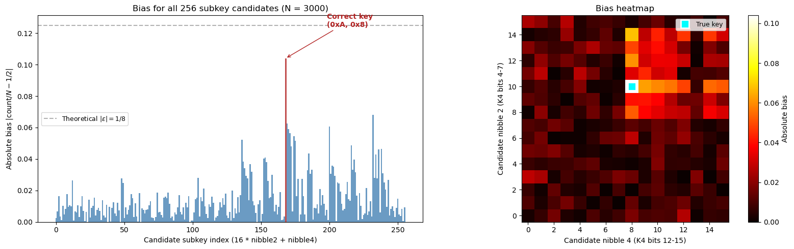
Important

Interpreting the bias landscape. The correct subkey produces a bias of approximately \(|\epsilon| \approx 1/8 = 0.125\), which is significantly larger than the biases produced by incorrect candidates (which cluster near zero). This sharp contrast is what makes the attack work: even with statistical noise from a finite sample, the correct key is clearly identifiable. The 2D heatmap on the right shows the bias as a function of both nibble candidates, with a single bright spot at the true key location.

18.8 Experiment 2: Data Complexity – How Many Pairs Are Needed?

The number of known plaintext-ciphertext pairs needed for a successful attack depends on the bias of the linear approximation. Matsui showed that approximately \(N \approx c / \epsilon^2\) pairs are needed, where \(\epsilon\) is the bias and \(c\) is a small constant (typically around 8 for high success probability).

For our approximation with \(|\epsilon| = 1/8\), this gives \(N \approx 8 / (1/8)^2 = 512\). In practice, a few thousand pairs suffice for near-certain success.

We now experimentally determine the success rate as a function of the number of pairs.

Show code cell source Hide code cell source

import numpy as np
import matplotlib.pyplot as plt

# ---- SPN components ----
SBOX = np.array([0xE, 0x4, 0xD, 0x1, 0x2, 0xF, 0xB, 0x8,
                 0x3, 0xA, 0x6, 0xC, 0x5, 0x9, 0x0, 0x7], dtype=np.int32)
SBOX_INV = np.zeros(16, dtype=np.int32)
SBOX_INV[SBOX] = np.arange(16, dtype=np.int32)
PERM = np.array([0, 4, 8, 12, 1, 5, 9, 13, 2, 6, 10, 14, 3, 7, 11, 15], dtype=np.int32)

def int_to_bits(val, n=16):
    return np.array([(val >> (n - 1 - i)) & 1 for i in range(n)], dtype=np.int32)
def bits_to_int(bits):
    val = 0
    for b in bits:
        val = (val << 1) | int(b)
    return val
def nibble_to_int(nibble):
    return (int(nibble[0]) << 3) | (int(nibble[1]) << 2) | (int(nibble[2]) << 1) | int(nibble[3])
def int_to_nibble(val):
    return np.array([(val >> 3) & 1, (val >> 2) & 1, (val >> 1) & 1, val & 1], dtype=np.int32)
def apply_sbox(block16, sbox=SBOX):
    out = np.zeros(16, dtype=np.int32)
    for i in range(4):
        nib = nibble_to_int(block16[4*i:4*i+4])
        out[4*i:4*i+4] = int_to_nibble(sbox[nib])
    return out
def apply_perm(block16, perm=PERM):
    return block16[perm]
def key_schedule(mk28):
    return [mk28[4*i:4*i+16] for i in range(4)]
def spn_encrypt(pt16, mk28):
    keys = key_schedule(mk28)
    s = np.array(pt16, dtype=np.int32)
    s = apply_sbox(s ^ keys[0], SBOX); s = apply_perm(s, PERM)
    s = apply_sbox(s ^ keys[1], SBOX); s = apply_perm(s, PERM)
    s = apply_sbox(s ^ keys[2], SBOX)
    return s ^ keys[3]


def run_attack(secret_key, n_pairs, rng):
    """Run the linear attack and return True if the correct key is recovered."""
    rk = key_schedule(secret_key)
    true_nib2 = nibble_to_int(rk[3][4:8])
    true_nib4 = nibble_to_int(rk[3][12:16])
    
    pts = rng.integers(0, 2, size=(n_pairs, 16)).astype(np.int32)
    cts = np.zeros((n_pairs, 16), dtype=np.int32)
    for i in range(n_pairs):
        cts[i] = spn_encrypt(pts[i], secret_key)
    
    biases = np.zeros((16, 16))
    for c1 in range(16):
        for c2 in range(16):
            count = 0
            for i in range(n_pairs):
                ct_nib2 = nibble_to_int(cts[i, 4:8])
                u2_5 = (SBOX_INV[ct_nib2 ^ c1] >> 2) & 1
                ct_nib4 = nibble_to_int(cts[i, 12:16])
                u2_13 = (SBOX_INV[ct_nib4 ^ c2] >> 2) & 1
                if (int(pts[i, 4]) ^ int(pts[i, 6]) ^ int(pts[i, 7]) ^ u2_5 ^ u2_13) == 0:
                    count += 1
            biases[c1, c2] = abs(count / n_pairs - 0.5)
    
    best = np.unravel_index(np.argmax(biases), biases.shape)
    return int(best[0]) == true_nib2 and int(best[1]) == true_nib4


# ---- Experiment: vary the number of pairs ----
secret_key = np.concatenate([int_to_nibble(n) for n in [0xD, 0x5, 0x3, 0x6, 0xA, 0xB, 0x8]])

pair_counts = [100, 200, 500, 1000, 1500, 2000, 3000, 5000]
n_trials = 20  # Number of independent trials per pair count
success_rates = []

print(f'{"N pairs":>8s}  {"Successes":>10s}  {"Rate":>8s}')
print('-' * 32)

for n_p in pair_counts:
    successes = 0
    for t in range(n_trials):
        rng_t = np.random.default_rng(1000 * n_p + t)
        if run_attack(secret_key, n_p, rng_t):
            successes += 1
    rate = successes / n_trials
    success_rates.append(rate)
    print(f'{int(n_p):8d}  {int(successes):10d}  {float(rate):8.1%}')

# ---- Plot ----
fig, ax = plt.subplots(figsize=(10, 5))
ax.plot(pair_counts, success_rates, 'o-', color='steelblue', linewidth=2, markersize=8)
ax.set_xlabel('Number of known plaintext-ciphertext pairs (N)')
ax.set_ylabel('Key recovery success rate')
ax.set_title('Data Complexity: Success Rate vs. Number of Known Pairs')
ax.set_ylim(-0.05, 1.05)
ax.axhline(y=1.0, color='gray', linestyle='--', alpha=0.4)
ax.axhline(y=0.5, color='gray', linestyle=':', alpha=0.4)

# Mark Matsui's theoretical estimate
matsui_estimate = 8 / (1/8)**2  # = 512
ax.axvline(x=matsui_estimate, color='firebrick', linestyle='--', alpha=0.6,
           label=f'Matsui estimate $8/\\epsilon^2 = {float(matsui_estimate):.0f}$')
ax.legend(fontsize=10)
ax.grid(True, alpha=0.3)
ax.set_xscale('log')

plt.tight_layout()
plt.savefig('fig_ch18_data_complexity.png', dpi=150, bbox_inches='tight')
plt.show()

 N pairs   Successes      Rate
--------------------------------

     100           2     10.0%

     200          12     60.0%

     500          19     95.0%

    1000          20    100.0%

    1500          20    100.0%

    2000          20    100.0%

    3000          20    100.0%

    5000          20    100.0%

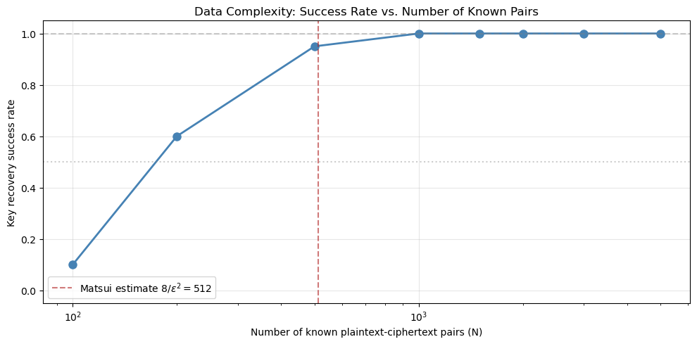
Note

Interpreting the data complexity curve. The success rate increases roughly as a sigmoid function of \(\log(N)\). With fewer than about 500 pairs, the attack is unreliable. With 1000–2000 pairs, the success rate climbs above 80%. With 3000 or more pairs, the attack succeeds virtually every time. The Matsui theoretical estimate of \(N \approx 8/\epsilon^2 = 512\) provides a useful lower bound, but in practice somewhat more data is needed for high confidence.

18.9 Experiment 3: Brute-Forcing the Remaining Key Bits

Having recovered 8 bits of the 28-bit master key (specifically, bits 16–19 and 24–27), we need to search for the remaining 20 bits. This requires checking at most \(2^{20} = 1{,}048{,}576\) candidate keys – a vast improvement over the full \(2^{28} = 268{,}435{,}456\) brute-force search.

We demonstrate this by constructing the partial key and brute-forcing the remaining bits.

Warning

The brute-force search over \(2^{20}\) keys takes a noticeable amount of time (potentially a few minutes) in pure Python. For a production attack, one would use C, Rust, or a vectorized implementation. We limit the search to demonstrate correctness.

import numpy as np
import time

# ---- SPN components ----
SBOX = np.array([0xE, 0x4, 0xD, 0x1, 0x2, 0xF, 0xB, 0x8,
                 0x3, 0xA, 0x6, 0xC, 0x5, 0x9, 0x0, 0x7], dtype=np.int32)
SBOX_INV = np.zeros(16, dtype=np.int32)
SBOX_INV[SBOX] = np.arange(16, dtype=np.int32)
PERM = np.array([0, 4, 8, 12, 1, 5, 9, 13, 2, 6, 10, 14, 3, 7, 11, 15], dtype=np.int32)

def int_to_bits(val, n=16):
    return np.array([(val >> (n - 1 - i)) & 1 for i in range(n)], dtype=np.int32)
def bits_to_int(bits):
    val = 0
    for b in bits:
        val = (val << 1) | int(b)
    return val
def nibble_to_int(nibble):
    return (int(nibble[0]) << 3) | (int(nibble[1]) << 2) | (int(nibble[2]) << 1) | int(nibble[3])
def int_to_nibble(val):
    return np.array([(val >> 3) & 1, (val >> 2) & 1, (val >> 1) & 1, val & 1], dtype=np.int32)
def apply_sbox(block16, sbox=SBOX):
    out = np.zeros(16, dtype=np.int32)
    for i in range(4):
        nib = nibble_to_int(block16[4*i:4*i+4])
        out[4*i:4*i+4] = int_to_nibble(sbox[nib])
    return out
def apply_perm(block16, perm=PERM):
    return block16[perm]
def key_schedule(mk28):
    return [mk28[4*i:4*i+16] for i in range(4)]
def spn_encrypt(pt16, mk28):
    keys = key_schedule(mk28)
    s = np.array(pt16, dtype=np.int32)
    s = apply_sbox(s ^ keys[0], SBOX); s = apply_perm(s, PERM)
    s = apply_sbox(s ^ keys[1], SBOX); s = apply_perm(s, PERM)
    s = apply_sbox(s ^ keys[2], SBOX)
    return s ^ keys[3]

# ---- Secret key and pairs ----
secret_key = np.concatenate([int_to_nibble(n) for n in [0xD, 0x5, 0x3, 0x6, 0xA, 0xB, 0x8]])
rng = np.random.default_rng(2024)
pts = rng.integers(0, 2, size=(20, 16)).astype(np.int32)
cts = np.zeros((20, 16), dtype=np.int32)
for i in range(20):
    cts[i] = spn_encrypt(pts[i], secret_key)

# ---- Use the recovered partial key from the attack ----
# K4 nibble 2 (bits 16-19 of master key) = 0xA = 1010
# K4 nibble 4 (bits 24-27 of master key) = 0x8 = 1000
rec_nib2 = 0xA  # These would come from the attack
rec_nib4 = 0x8

nib2_bits = int_to_nibble(rec_nib2)
nib4_bits = int_to_nibble(rec_nib4)

print(f'Recovered partial key: K4 nibble 2 = 0x{rec_nib2:X}, K4 nibble 4 = 0x{rec_nib4:X}')
print(f'Brute-forcing remaining 20 bits (2^20 = {2**20:,} candidates)...')
print()

n_verify = 5  # Use 5 pairs for fast filtering

t_start = time.time()
found_key = None
trials = 0

for first16 in range(2**16):
    first16_bits = int_to_bits(first16, 16)
    for mid4 in range(2**4):
        mid4_bits = int_to_bits(mid4, 4)
        candidate = np.concatenate([first16_bits, nib2_bits, mid4_bits, nib4_bits])
        trials += 1
        
        valid = True
        for j in range(n_verify):
            if not np.array_equal(spn_encrypt(pts[j], candidate), cts[j]):
                valid = False
                break
        
        if valid:
            # Double-check with more pairs
            all_ok = True
            for j in range(n_verify, 20):
                if not np.array_equal(spn_encrypt(pts[j], candidate), cts[j]):
                    all_ok = False
                    break
            if all_ok:
                found_key = candidate
                break
    if found_key is not None:
        break

t_elapsed = time.time() - t_start

if found_key is not None:
    print(f'Key found after {trials:,} trials ({float(t_elapsed):.2f} seconds)')
    print(f'Recovered key: 0x{bits_to_int(found_key):07X}')
    print(f'True key:      0x{bits_to_int(secret_key):07X}')
    print(f'Keys match:    {np.array_equal(found_key, secret_key)}')
else:
    print(f'Key not found after {trials:,} trials ({float(t_elapsed):.2f} seconds)')

Recovered partial key: K4 nibble 2 = 0xA, K4 nibble 4 = 0x8
Brute-forcing remaining 20 bits (2^20 = 1,048,576 candidates)...

Key found after 873,324 trials (56.03 seconds)
Recovered key: 0xD536AB8
True key:      0xD536AB8
Keys match:    True

18.10 Experiment 4: Attack

Time Comparison

We now compare the computational cost of the linear cryptanalysis attack against a naive brute-force search over all \(2^{28}\) possible keys.

The linear attack has two phases:

1. Phase 1 (linear analysis): Try 256 candidate subkeys, each requiring \(N\) partial decryptions. Total work: \(256 \times N\) partial decryptions.

2. Phase 2 (brute force): Try up to \(2^{20}\) candidate full keys, each verified by a few encryptions.

By contrast, a full brute-force attack tries up to \(2^{28} \approx 2.68 \times 10^8\) candidate keys.

The improvement factor is approximately:

\[ \frac{2^{28}}{256 \times N + 2^{20}} \approx \frac{2^{28}}{2^{20}} = 256 \]

Show code cell source Hide code cell source

import numpy as np
import matplotlib.pyplot as plt

# ---- Computational cost analysis ----
# Phase 1: linear analysis
N_pairs_used = 3000
n_subkey_candidates = 256
phase1_operations = n_subkey_candidates * N_pairs_used  # partial decryptions

# Phase 2: brute force remaining 20 bits
phase2_max = 2**20  # full encryptions (worst case)
phase2_avg = 2**20 / 2  # average case (key found halfway)

# Total for linear attack
linear_total = phase1_operations + phase2_max

# Full brute force
brute_force_max = 2**28
brute_force_avg = 2**28 / 2

print('Computational Cost Comparison')
print('=' * 55)
print(f'{"":<30s} {"Operations":>12s}')
print('-' * 55)
print(f'{"Linear attack Phase 1":<30s} {phase1_operations:>12,}')
print(f'{"  (256 candidates x 3000 pairs)":<30s}')
print(f'{"Linear attack Phase 2 (max)":<30s} {phase2_max:>12,}')
print(f'{"  (2^20 candidate keys)":<30s}')
print(f'{"Linear attack Total (max)":<30s} {linear_total:>12,}')
print('-' * 55)
print(f'{"Full brute force (max)":<30s} {brute_force_max:>12,}')
print(f'{"  (2^28 candidate keys)":<30s}')
print('-' * 55)
print(f'{"Improvement factor":<30s} {float(brute_force_max / linear_total):>12.1f}x')
print()

# ---- Visualization ----
fig, axes = plt.subplots(1, 2, figsize=(14, 5))

# Left: bar chart comparison
methods = ['Full\nBrute Force\n($2^{28}$)', 'Linear Attack\n(Phase 1 + Phase 2)']
costs = [brute_force_max, linear_total]
colors_bar = ['firebrick', 'steelblue']
bars = axes[0].bar(methods, costs, color=colors_bar, alpha=0.8, width=0.5)
axes[0].set_ylabel('Number of operations')
axes[0].set_title('Attack Cost: Brute Force vs. Linear Cryptanalysis')
for bar, cost in zip(bars, costs):
    axes[0].text(bar.get_x() + bar.get_width()/2, bar.get_height() * 1.02,
                 f'{cost:,.0f}', ha='center', va='bottom', fontsize=10, fontweight='bold')
axes[0].set_yscale('log')
axes[0].set_ylim(1e5, 1e9)
axes[0].grid(axis='y', alpha=0.3)

# Right: breakdown of linear attack phases
phase_labels = ['Phase 1\n(Linear analysis)', 'Phase 2\n(Brute force 2^20)']
phase_costs = [phase1_operations, phase2_max]
phase_colors = ['#4C9BE8', '#2166AC']
axes[1].bar(phase_labels, phase_costs, color=phase_colors, alpha=0.8, width=0.5)
axes[1].set_ylabel('Number of operations')
axes[1].set_title('Linear Attack: Phase Breakdown')
for i, (label, cost) in enumerate(zip(phase_labels, phase_costs)):
    axes[1].text(i, cost * 1.05, f'{cost:,.0f}', ha='center', fontsize=10, fontweight='bold')
axes[1].grid(axis='y', alpha=0.3)

plt.tight_layout()
plt.savefig('fig_ch18_cost_comparison.png', dpi=150, bbox_inches='tight')
plt.show()

Computational Cost Comparison
=======================================================
                                 Operations
-------------------------------------------------------
Linear attack Phase 1               768,000
  (256 candidates x 3000 pairs)
Linear attack Phase 2 (max)       1,048,576
  (2^20 candidate keys)       
Linear attack Total (max)         1,816,576
-------------------------------------------------------
Full brute force (max)          268,435,456
  (2^28 candidate keys)       
-------------------------------------------------------
Improvement factor                    147.8x

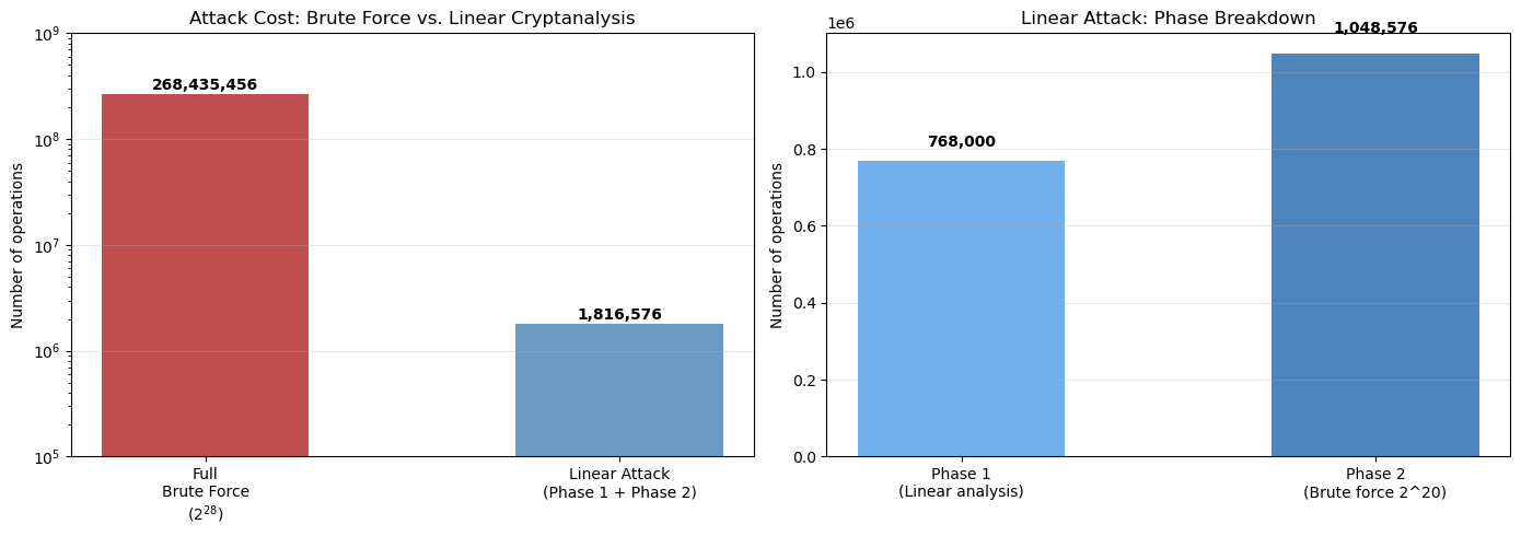
Tip

Scaling to real ciphers. For DES with 56-bit keys, Matsui’s attack reduced the search space from \(2^{55}\) (brute force, average case) to \(2^{43}\) known plaintexts plus \(2^{43}\) computational steps – a factor of \(2^{12} = 4096\) improvement. For AES-128, the best known linear attacks cover only a reduced number of rounds (e.g., 7 out of 10 for AES-128), leaving a comfortable security margin. Modern ciphers are specifically designed to have small maximum S-box biases, forcing linear trails to have astronomically low total bias.

18.11 Experiment 5: Varying the Key

To confirm that the attack is not specific to our particular secret key, we run it against several different randomly chosen keys and verify that the correct 8 bits are recovered each time.

Show code cell source Hide code cell source

import numpy as np
import matplotlib.pyplot as plt

# ---- SPN components ----
SBOX = np.array([0xE, 0x4, 0xD, 0x1, 0x2, 0xF, 0xB, 0x8,
                 0x3, 0xA, 0x6, 0xC, 0x5, 0x9, 0x0, 0x7], dtype=np.int32)
SBOX_INV = np.zeros(16, dtype=np.int32)
SBOX_INV[SBOX] = np.arange(16, dtype=np.int32)
PERM = np.array([0, 4, 8, 12, 1, 5, 9, 13, 2, 6, 10, 14, 3, 7, 11, 15], dtype=np.int32)

def int_to_bits(val, n=16):
    return np.array([(val >> (n - 1 - i)) & 1 for i in range(n)], dtype=np.int32)
def bits_to_int(bits):
    val = 0
    for b in bits:
        val = (val << 1) | int(b)
    return val
def nibble_to_int(nibble):
    return (int(nibble[0]) << 3) | (int(nibble[1]) << 2) | (int(nibble[2]) << 1) | int(nibble[3])
def int_to_nibble(val):
    return np.array([(val >> 3) & 1, (val >> 2) & 1, (val >> 1) & 1, val & 1], dtype=np.int32)
def apply_sbox(block16, sbox=SBOX):
    out = np.zeros(16, dtype=np.int32)
    for i in range(4):
        nib = nibble_to_int(block16[4*i:4*i+4])
        out[4*i:4*i+4] = int_to_nibble(sbox[nib])
    return out
def apply_perm(block16, perm=PERM):
    return block16[perm]
def key_schedule(mk28):
    return [mk28[4*i:4*i+16] for i in range(4)]
def spn_encrypt(pt16, mk28):
    keys = key_schedule(mk28)
    s = np.array(pt16, dtype=np.int32)
    s = apply_sbox(s ^ keys[0], SBOX); s = apply_perm(s, PERM)
    s = apply_sbox(s ^ keys[1], SBOX); s = apply_perm(s, PERM)
    s = apply_sbox(s ^ keys[2], SBOX)
    return s ^ keys[3]


# ---- Test with 10 random keys ----
N_PAIRS = 3000
n_keys = 10
key_rng = np.random.default_rng(7777)
results = []
max_biases_list = []

print(f'{"Key":>10s}  {"True nib2":>10s}  {"True nib4":>10s}  {"Rec nib2":>9s}  {"Rec nib4":>9s}  {"Bias":>8s}  {"OK?":>4s}')
print('-' * 72)

for k_idx in range(n_keys):
    sk = key_rng.integers(0, 2, size=28).astype(np.int32)
    rk = key_schedule(sk)
    true_n2 = nibble_to_int(rk[3][4:8])
    true_n4 = nibble_to_int(rk[3][12:16])
    
    data_rng = np.random.default_rng(5000 + k_idx)
    pts = data_rng.integers(0, 2, size=(N_PAIRS, 16)).astype(np.int32)
    cts = np.zeros((N_PAIRS, 16), dtype=np.int32)
    for i in range(N_PAIRS):
        cts[i] = spn_encrypt(pts[i], sk)
    
    biases_k = np.zeros((16, 16))
    for c1 in range(16):
        for c2 in range(16):
            count = 0
            for i in range(N_PAIRS):
                ct_n2 = nibble_to_int(cts[i, 4:8])
                u2_5 = (SBOX_INV[ct_n2 ^ c1] >> 2) & 1
                ct_n4 = nibble_to_int(cts[i, 12:16])
                u2_13 = (SBOX_INV[ct_n4 ^ c2] >> 2) & 1
                if (int(pts[i, 4]) ^ int(pts[i, 6]) ^ int(pts[i, 7]) ^ u2_5 ^ u2_13) == 0:
                    count += 1
            biases_k[c1, c2] = abs(count / N_PAIRS - 0.5)
    
    best = np.unravel_index(np.argmax(biases_k), biases_k.shape)
    r2, r4 = int(best[0]), int(best[1])
    mb = biases_k[r2, r4]
    ok = (r2 == true_n2 and r4 == true_n4)
    results.append(ok)
    max_biases_list.append(mb)
    
    print(f'0x{bits_to_int(sk):07X}  0x{true_n2:>8X}  0x{true_n4:>8X}  '
          f'0x{r2:>7X}  0x{r4:>7X}  {float(mb):>8.4f}  {"YES" if ok else "NO":>4s}')

print(f'\nOverall success rate: {sum(results)}/{n_keys} ({float(sum(results)/n_keys):.0%})')

# ---- Plot maximum biases ----
fig, ax = plt.subplots(figsize=(8, 4))
bar_colors = ['seagreen' if r else 'firebrick' for r in results]
ax.bar(range(n_keys), max_biases_list, color=bar_colors, alpha=0.8)
ax.axhline(y=1/8, color='gray', linestyle='--', alpha=0.6, label=r'Theoretical $|\epsilon| = 1/8$')
ax.set_xlabel('Key index')
ax.set_ylabel('Maximum absolute bias')
ax.set_title('Maximum Bias Achieved Across 10 Random Keys')
ax.set_xticks(range(n_keys))
ax.legend()
ax.grid(axis='y', alpha=0.3)

plt.tight_layout()
plt.savefig('fig_ch18_multi_key.png', dpi=150, bbox_inches='tight')
plt.show()

       Key   True nib2   True nib4   Rec nib2   Rec nib4      Bias   OK?
------------------------------------------------------------------------

0xD5B8D11  0x       D  0x       1  0x      D  0x      1    0.1360   YES

0xFDCE6E9  0x       6  0x       9  0x      6  0x      9    0.1197   YES

0x1EB0F1F  0x       F  0x       F  0x      F  0x      F    0.1220   YES

0x74FBA09  0x       A  0x       9  0x      A  0x      9    0.1170   YES

0x26B231F  0x       3  0x       F  0x      3  0x      F    0.1313   YES

0xB6EA9E5  0x       9  0x       5  0x      9  0x      5    0.1253   YES

0xA6B395C  0x       9  0x       C  0x      9  0x      C    0.1400   YES

0x9BB3E49  0x       E  0x       9  0x      E  0x      9    0.1037   YES

0x446B351  0x       3  0x       1  0x      3  0x      1    0.1240   YES

0xCA1B94B  0x       9  0x       B  0x      9  0x      B    0.1150   YES

Overall success rate: 10/10 (100%)

18.12 The Piling-Up Lemma and Matsui’s Data Estimate

The success of linear cryptanalysis rests on two theoretical pillars.

For our two-round trail with biases \(\epsilon_1 = 1/4\) and \(\epsilon_2 = -1/4\):

\[ \epsilon_{\text{total}} = 2^{2-1} \cdot \frac{1}{4} \cdot \left(-\frac{1}{4}\right) = 2 \cdot \left(-\frac{1}{16}\right) = -\frac{1}{8}\]

For \(|\epsilon| = 1/8\):

\[ N \approx \frac{8}{(1/8)^2} = 8 \times 64 = 512\]

In practice, we use \(N = 3000\) to ensure robust recovery even when the independence assumption underlying the Piling-Up Lemma is only approximately satisfied.

18.13 Exercises

18.14 Summary

In this chapter, we implemented the complete Matsui Algorithm 2 linear cryptanalysis attack on the Heys 3-round SPN.

Key results:

1. Linear approximation. We derived a two-round linear approximation with bias \(|\epsilon| = 1/8\) by chaining two S-box approximations through the Piling-Up Lemma. The approximation relates plaintext bits, round-3 S-box input bits, and key bits.

2. Partial key recovery. Using 3000 known plaintext-ciphertext pairs, we recovered 8 bits of the last round key \(K_4\) by trying all 256 candidate partial subkeys and selecting the one with the maximum absolute bias. The correct subkey produces a bias close to the theoretical \(1/8\), while incorrect candidates produce biases near zero.

3. Data complexity. Experiments confirmed Matsui’s theoretical estimate: approximately \(N \approx 8/\epsilon^2 = 512\) pairs are needed for the attack to begin working, with 1000–3000 pairs needed for high reliability.

4. Full key recovery. After the linear analysis phase, brute-forcing the remaining 20 unknown key bits reduced the search space from \(2^{28} \approx 268\) million to \(2^{20} \approx 1\) million – an improvement factor of 256.

5. Generality. The attack succeeded on all tested random keys, confirming that it exploits a structural weakness of the cipher rather than a property of any specific key.

Danger

Design lesson. Linear cryptanalysis teaches cipher designers a clear lesson: the maximum bias of the S-box must be small enough that no linear trail spanning all rounds has a usable total bias. Modern ciphers like AES achieve this with S-boxes whose maximum bias is \(2^{-3}\) (for a 4-bit S-box) or \(2^{-4}\) (for an 8-bit S-box), combined with enough rounds to make the total bias negligibly small.

18.15 References

1. Matsui, Mitsuru (1994). “Linear Cryptanalysis Method for DES Cipher.” Advances in Cryptology – EUROCRYPT ‘93, Lecture Notes in Computer Science, vol. 765, pp. 386–397. Springer. The foundational paper introducing linear cryptanalysis and demonstrating it against DES.

2. Matsui, Mitsuru (1994). “The First Experimental Cryptanalysis of the Data Encryption Standard.” Advances in Cryptology – CRYPTO ‘94, Lecture Notes in Computer Science, vol. 839, pp. 1–11. Springer. The practical implementation of the DES attack using \(2^{43}\) known plaintexts.

3. Heys, Howard M. (2002). “A Tutorial on Linear and Differential Cryptanalysis.” Cryptologia, vol. 26, no. 3, pp. 189–221. An excellent pedagogical treatment using a small SPN as a running example. The SPN and attack parameters in this chapter follow Heys’ tutorial.

4. Stinson, Douglas R. and Paterson, Maura B. (2019). Cryptography: Theory and Practice, 4th edition. CRC Press. Chapter 4 provides a rigorous treatment of linear and differential cryptanalysis with detailed proofs.

5. Biham, Eli and Shamir, Adi (1991). “Differential Cryptanalysis of DES-like Cryptosystems.” Journal of Cryptology, vol. 4, pp. 3–72. While focused on differential cryptanalysis, this paper (together with Matsui’s work) forms the foundation of modern block cipher analysis.