Chapter 31: PyTorch CNN on MNIST#
In Chapters 23-25 we built a convolutional neural network from scratch in NumPy
on \(8 \times 8\) synthetic patterns. Our TinyCNN class implemented convolution,
ReLU, max pooling, and a fully connected classifier – all with hand-written
forward and backward passes. The exercise was invaluable for understanding the
mechanics of CNNs, but the implementation was slow and limited to tiny images.
Now we rebuild the same architecture in PyTorch and train it on the full MNIST dataset – 60,000 images of \(28 \times 28\) pixels. Where our NumPy CNN took minutes to train on 200 synthetic samples, PyTorch will process millions of images with automatic differentiation, optimized BLAS routines, and (optionally) GPU acceleration.
The conceptual leap is small – we already understand every layer – but the practical leap is enormous.
Show code cell source
import numpy as np
import matplotlib.pyplot as plt
import torch
import torch.nn as nn
import torch.optim as optim
import torch.nn.functional as F
from torch.utils.data import DataLoader
import torchvision
import torchvision.transforms as transforms

# Consistent style for all plots
plt.rcParams.update({
    'figure.dpi': 100,
    'font.size': 11,
    'axes.titlesize': 13,
    'axes.labelsize': 12
})

# Standard color palette
BLUE = '#3b82f6'
GREEN = '#059669'
RED = '#dc2626'
AMBER = '#d97706'
INDIGO = '#4f46e5'

torch.manual_seed(42)
device = torch.device('cuda' if torch.cuda.is_available() else 'cpu')
print(f'PyTorch version: {torch.__version__}')
print(f'Device: {device}')
PyTorch version: 2.7.0
Device: cpu
31.1 From TinyCNN to PyTorch#
Recall the architecture of our NumPy TinyCNN from Chapter 23:
Conv2D: 1 input channel, 4 filters of size \(3 \times 3\)
ReLU: element-wise activation
MaxPool: \(2 \times 2\) pooling with stride 2
Flatten: reshape to a vector
Dense: fully connected to 2 output classes
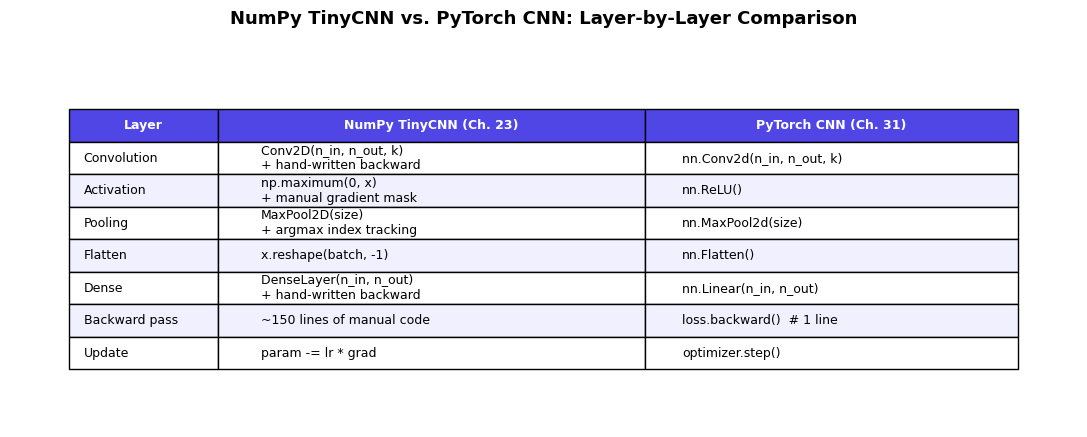
Each of these required 50-100 lines of careful NumPy code for both forward and backward passes. In PyTorch, the same architecture is a few lines.
The following table shows the exact correspondence:
Show code cell source
# --- Side-by-side comparison table ---
fig, ax = plt.subplots(figsize=(11, 4.5))
ax.axis('off')

table_data = [
    ['Layer', 'NumPy TinyCNN (Ch. 23)', 'PyTorch CNN (Ch. 31)'],
    ['Convolution', 'Conv2D(n_in, n_out, k)\n+ hand-written backward', 'nn.Conv2d(n_in, n_out, k)'],
    ['Activation', 'np.maximum(0, x)\n+ manual gradient mask', 'nn.ReLU()'],
    ['Pooling', 'MaxPool2D(size)\n+ argmax index tracking', 'nn.MaxPool2d(size)'],
    ['Flatten', 'x.reshape(batch, -1)', 'nn.Flatten()'],
    ['Dense', 'DenseLayer(n_in, n_out)\n+ hand-written backward', 'nn.Linear(n_in, n_out)'],
    ['Backward pass', '~150 lines of manual code', 'loss.backward()  # 1 line'],
    ['Update', 'param -= lr * grad', 'optimizer.step()'],
]

table = ax.table(cellText=table_data[1:], colLabels=table_data[0],
                 cellLoc='left', loc='center',
                 colWidths=[0.14, 0.40, 0.35])
table.auto_set_font_size(False)
table.set_fontsize(9)
table.scale(1.0, 1.8)

# Style header
for j in range(3):
    table[0, j].set_facecolor(INDIGO)
    table[0, j].set_text_props(color='white', fontweight='bold')

# Alternate row colors
for i in range(1, len(table_data)):
    color = '#f0f0ff' if i % 2 == 0 else 'white'
    for j in range(3):
        table[i, j].set_facecolor(color)

ax.set_title('NumPy TinyCNN vs. PyTorch CNN: Layer-by-Layer Comparison',
             fontsize=13, fontweight='bold', pad=20)
plt.tight_layout()
plt.show()
The Key Insight
The conceptual content is identical – both implementations perform the same mathematical operations. But PyTorch’s autograd eliminates the need to manually derive and implement backward passes for each layer. This is exactly the shift from Chapter 28 (manual backprop) to Chapter 29 (autograd): the mathematics stays the same, but the engineering burden drops dramatically.
31.2 Training on Full MNIST#
We scale up from the TinyCNN’s 4 filters on \(8 \times 8\) images to a proper architecture for \(28 \times 28\) MNIST digits:
Let us trace the dimensions through the network:
Input: \((B, 1, 28, 28)\)
After Conv1 (\(3 \times 3\), 16 filters): \((B, 16, 26, 26)\)
After Pool1 (\(2 \times 2\)): \((B, 16, 13, 13)\)
After Conv2 (\(3 \times 3\), 32 filters): \((B, 32, 11, 11)\)
After Pool2 (\(2 \times 2\)): \((B, 32, 5, 5)\)
After Flatten: \((B, 800)\)
After Linear: \((B, 10)\)
# --- Define the CNN ---
class MNISTCNN(nn.Module):
    """Two-layer CNN for MNIST, extending TinyCNN (Ch. 23) to full scale."""

    def __init__(self):
        super().__init__()
        # Feature extraction (cf. TinyCNN's conv + pool)
        self.conv1 = nn.Conv2d(1, 16, kernel_size=3)    # 28x28 -> 26x26
        self.conv2 = nn.Conv2d(16, 32, kernel_size=3)   # 13x13 -> 11x11
        self.pool = nn.MaxPool2d(2, 2)                   # halve spatial dims

        # Classifier (cf. TinyCNN's dense layer)
        self.flatten = nn.Flatten()
        self.fc = nn.Linear(32 * 5 * 5, 10)

    def forward(self, x):
        x = self.pool(F.relu(self.conv1(x)))   # (B,1,28,28) -> (B,16,13,13)
        x = self.pool(F.relu(self.conv2(x)))   # (B,16,13,13) -> (B,32,5,5)
        x = self.flatten(x)                     # (B,32,5,5) -> (B,800)
        x = self.fc(x)                          # (B,800) -> (B,10)
        return x

torch.manual_seed(42)
cnn_model = MNISTCNN().to(device)
print(cnn_model)

n_params = sum(p.numel() for p in cnn_model.parameters())
print(f'\nTotal parameters: {n_params:,}')

# Verify dimensions with a dummy input
dummy = torch.randn(1, 1, 28, 28).to(device)
out = cnn_model(dummy)
print(f'Input shape:  {dummy.shape}')
print(f'Output shape: {out.shape}')
MNISTCNN(
  (conv1): Conv2d(1, 16, kernel_size=(3, 3), stride=(1, 1))
  (conv2): Conv2d(16, 32, kernel_size=(3, 3), stride=(1, 1))
  (pool): MaxPool2d(kernel_size=2, stride=2, padding=0, dilation=1, ceil_mode=False)
  (flatten): Flatten(start_dim=1, end_dim=-1)
  (fc): Linear(in_features=800, out_features=10, bias=True)
)

Total parameters: 12,810
Input shape:  torch.Size([1, 1, 28, 28])
Output shape: torch.Size([1, 10])
# --- Load MNIST data ---
transform = transforms.Compose([
    transforms.ToTensor(),
    transforms.Normalize((0.1307,), (0.3081,))
])

train_dataset = torchvision.datasets.MNIST(
    root='./data', train=True, download=True, transform=transform
)
test_dataset = torchvision.datasets.MNIST(
    root='./data', train=False, download=True, transform=transform
)

train_loader = DataLoader(train_dataset, batch_size=64, shuffle=True)
test_loader = DataLoader(test_dataset, batch_size=64, shuffle=False)

print(f'Training batches: {len(train_loader)}')
print(f'Test batches: {len(test_loader)}')
Training batches: 938
Test batches: 157
# --- Train the CNN ---
torch.manual_seed(42)
cnn_model = MNISTCNN().to(device)
loss_fn = nn.CrossEntropyLoss()
optimizer = optim.Adam(cnn_model.parameters(), lr=0.001)

cnn_train_losses = []
cnn_test_accuracies = []
n_epochs = 5

for epoch in range(n_epochs):
    # Training
    cnn_model.train()
    epoch_loss = 0.0
    n_batches = 0

    for X_batch, y_batch in train_loader:
        X_batch, y_batch = X_batch.to(device), y_batch.to(device)

        pred = cnn_model(X_batch)
        loss = loss_fn(pred, y_batch)

        optimizer.zero_grad()
        loss.backward()
        optimizer.step()

        epoch_loss += loss.item()
        n_batches += 1

    avg_loss = epoch_loss / n_batches
    cnn_train_losses.append(avg_loss)

    # Evaluation
    cnn_model.eval()
    correct = 0
    total = 0
    with torch.no_grad():
        for X_batch, y_batch in test_loader:
            X_batch, y_batch = X_batch.to(device), y_batch.to(device)
            pred = cnn_model(X_batch)
            _, predicted = torch.max(pred, 1)
            total += y_batch.size(0)
            correct += (predicted == y_batch).sum().item()

    accuracy = 100.0 * correct / total
    cnn_test_accuracies.append(accuracy)

    print(f'Epoch {epoch+1}/{n_epochs} -- '
          f'Train Loss: {avg_loss:.4f}, '
          f'Test Accuracy: {accuracy:.2f}%')

print(f'\nFinal CNN test accuracy: {cnn_test_accuracies[-1]:.2f}%')
Epoch 1/5 -- Train Loss: 0.1924, Test Accuracy: 97.88%
Epoch 2/5 -- Train Loss: 0.0637, Test Accuracy: 98.51%
Epoch 3/5 -- Train Loss: 0.0473, Test Accuracy: 98.67%
Epoch 4/5 -- Train Loss: 0.0394, Test Accuracy: 98.60%
Epoch 5/5 -- Train Loss: 0.0337, Test Accuracy: 98.75%

Final CNN test accuracy: 98.75%
Show code cell source
# --- Plot training curves ---
fig, (ax1, ax2) = plt.subplots(1, 2, figsize=(12, 4))

# Loss curve
ax1.plot(range(1, n_epochs + 1), cnn_train_losses, 'o-', color=INDIGO,
         linewidth=2, markersize=8)
ax1.set_xlabel('Epoch')
ax1.set_ylabel('Training Loss')
ax1.set_title('CNN Training Loss', fontweight='bold')
ax1.grid(True, alpha=0.3)
ax1.set_xticks(range(1, n_epochs + 1))

# Accuracy curve
ax2.plot(range(1, n_epochs + 1), cnn_test_accuracies, 'o-', color=GREEN,
         linewidth=2, markersize=8)
ax2.set_xlabel('Epoch')
ax2.set_ylabel('Test Accuracy (%)')
ax2.set_title('CNN Test Accuracy', fontweight='bold')
ax2.grid(True, alpha=0.3)
ax2.set_xticks(range(1, n_epochs + 1))
ax2.set_ylim(95, 100)
ax2.axhline(y=98, color=RED, linestyle='--', alpha=0.5, label='98% target')
ax2.legend()

fig.suptitle('MNIST CNN Training (Conv16-Conv32-FC10)',
             fontsize=14, fontweight='bold')
plt.tight_layout()
plt.show()

CNN vs. MLP
Compare the CNN’s accuracy (~98-99%) with the MLP’s (~97%) from Chapter 30. The CNN achieves better performance with fewer parameters because convolutional layers exploit the spatial structure of images – exactly the motivation we discussed in Chapter 21 (translation invariance, local connectivity, weight sharing).
31.3 Learned Filters#
In Chapter 25, we visualized the learned filters of our NumPy TinyCNN and observed that they resembled edge detectors. Let us perform the same analysis on our PyTorch CNN’s first convolutional layer.
# --- Extract and inspect first-layer filters ---
filters = cnn_model.conv1.weight.data.cpu().numpy()
print(f'First-layer filter shape: {filters.shape}')  # (16, 1, 3, 3)
print(f'Number of filters: {filters.shape[0]}')
print(f'Filter size: {filters.shape[2]}x{filters.shape[3]}')
print(f'Value range: [{filters.min():.3f}, {filters.max():.3f}]')
First-layer filter shape: (16, 1, 3, 3)
Number of filters: 16
Filter size: 3x3
Value range: [-0.702, 0.590]
Show code cell source
# --- Visualize all 16 first-layer filters ---
fig, axes = plt.subplots(2, 8, figsize=(14, 4))

vmax = max(abs(filters.min()), abs(filters.max()))

for i, ax in enumerate(axes.flat):
    kernel = filters[i, 0]  # shape: (3, 3)
    im = ax.imshow(kernel, cmap='RdBu_r', vmin=-vmax, vmax=vmax,
                   interpolation='nearest')
    ax.set_title(f'Filter {i}', fontsize=9)
    ax.axis('off')

fig.suptitle('Learned First-Layer Convolution Filters (cf. Ch. 25 TinyCNN)',
             fontsize=14, fontweight='bold')
fig.colorbar(im, ax=axes, fraction=0.02, pad=0.04, label='Weight')
plt.tight_layout()
plt.show()
/var/folders/z7/wp7m8p7x1250jzvklw5z24mm0000gn/T/ipykernel_16722/3214114284.py:16: UserWarning: This figure includes Axes that are not compatible with tight_layout, so results might be incorrect.
  plt.tight_layout()
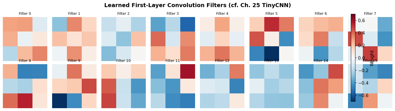
Interpreting the Filters
The first-layer filters learn to detect simple visual features: horizontal edges, vertical edges, diagonal edges, and simple gradients. This matches what we observed in Chapter 25 with TinyCNN and aligns with the classical findings of Hubel and Wiesel (1962) on simple cells in the cat visual cortex. The network has independently discovered edge detection as the optimal first processing step for digit recognition.
Show code cell source
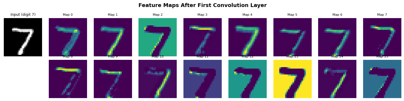
# --- Visualize feature maps for a sample digit ---
sample_img, sample_label = test_dataset[0]
sample_img = sample_img.unsqueeze(0).to(device)  # (1, 1, 28, 28)

# Get activations after first conv layer
cnn_model.eval()
with torch.no_grad():
    conv1_out = F.relu(cnn_model.conv1(sample_img))  # (1, 16, 26, 26)

conv1_maps = conv1_out[0].cpu().numpy()  # (16, 26, 26)

fig, axes = plt.subplots(2, 9, figsize=(14, 3.5))

# Original image
axes[0, 0].imshow(sample_img[0, 0].cpu(), cmap='gray')
axes[0, 0].set_title(f'Input (digit {sample_label})', fontsize=9)
axes[0, 0].axis('off')
axes[1, 0].axis('off')

# Feature maps
for i in range(16):
    row = i // 8
    col = i % 8 + 1
    axes[row, col].imshow(conv1_maps[i], cmap='viridis')
    axes[row, col].set_title(f'Map {i}', fontsize=8)
    axes[row, col].axis('off')

fig.suptitle('Feature Maps After First Convolution Layer',
             fontsize=13, fontweight='bold')
plt.tight_layout()
plt.show()
31.4 Pretrained Models Preview#
Our MNIST CNN has ~13,000 parameters and achieves ~98-99% accuracy on a simple benchmark. In practice, modern computer vision uses much larger architectures pretrained on millions of images.
PyTorch’s torchvision.models provides ready-to-use architectures:
Model |
Year |
Parameters |
ImageNet Top-1 |
|---|---|---|---|
AlexNet |
2012 |
61M |
56.5% |
VGG-16 |
2014 |
138M |
71.6% |
ResNet-50 |
2015 |
25M |
76.1% |
EfficientNet-B0 |
2019 |
5.3M |
77.1% |
ViT-B/16 |
2020 |
86M |
77.9% |
Transfer Learning
A pretrained model’s early layers learn universal visual features (edges, textures, shapes) that transfer across tasks. Fine-tuning – replacing the final classification layer and training on a new dataset – often achieves excellent results with very little data. We will explore transfer learning in detail in a later chapter.
# --- Preview: listing available pretrained models ---
# We only inspect the API here; downloading pretrained weights is deferred
# to the transfer learning chapter.

print('Selected torchvision.models architectures:')
selected_models = ['resnet18', 'resnet50', 'vgg16', 'mobilenet_v2', 'efficientnet_b0']
for name in selected_models:
    model_fn = getattr(torchvision.models, name)
    m = model_fn(weights=None)  # no pretrained weights
    n_params = sum(p.numel() for p in m.parameters())
    print(f'  {name:25s} -- {n_params:>12,} parameters')
Selected torchvision.models architectures:
  resnet18                  --   11,689,512 parameters
resnet50 -- 25,557,032 parameters
  vgg16                     --  138,357,544 parameters
  mobilenet_v2              --    3,504,872 parameters
  efficientnet_b0           --    5,288,548 parameters
31.5 Framework Corner: Same CNN in Other Frameworks#
The Same Architecture in TensorFlow/Keras and JAX/Flax
TensorFlow/Keras:
import tensorflow as tf

model = tf.keras.Sequential([
    tf.keras.layers.Conv2D(16, 3, activation='relu', input_shape=(28, 28, 1)),
    tf.keras.layers.MaxPooling2D(2),
    tf.keras.layers.Conv2D(32, 3, activation='relu'),
    tf.keras.layers.MaxPooling2D(2),
    tf.keras.layers.Flatten(),
    tf.keras.layers.Dense(10),
])
model.compile(optimizer='adam',
              loss=tf.keras.losses.SparseCategoricalCrossentropy(from_logits=True),
              metrics=['accuracy'])
model.fit(x_train, y_train, epochs=5, batch_size=64)
Note: Keras uses channels-last format (H, W, C) by default, while PyTorch uses channels-first (C, H, W).
JAX/Flax:
import jax
import jax.numpy as jnp
from flax import linen as fnn

class MNISTCNN(fnn.Module):
    @fnn.compact
    def __call__(self, x):
        x = fnn.Conv(16, (3, 3))(x)
        x = fnn.relu(x)
        x = fnn.max_pool(x, (2, 2), strides=(2, 2))
        x = fnn.Conv(32, (3, 3))(x)
        x = fnn.relu(x)
        x = fnn.max_pool(x, (2, 2), strides=(2, 2))
        x = x.reshape((x.shape[0], -1))
        x = fnn.Dense(10)(x)
        return x
Flax follows a functional paradigm: parameters are passed explicitly rather than stored in the model object. This makes JAX models pure functions, enabling jit, grad, and vmap transformations.
All three frameworks implement the same mathematical operations. The choice between them is primarily about API preference and ecosystem:
PyTorch: dominant in research, imperative style
TensorFlow/Keras: strong in deployment (TF Lite, TF Serving)
JAX/Flax: functional, composable transformations, Google TPU integration
Exercises#
Exercise 31.1. Add a third convolutional layer Conv2d(32, 64, 3) with ReLU and
max pooling between conv2 and the fully connected layer. Compute the new flattened
dimension by tracing shapes through the network. Does the additional layer improve
test accuracy? How many additional parameters does it add?
Exercise 31.2. Replace nn.MaxPool2d with nn.AvgPool2d (average pooling) in
the CNN. Train for 5 epochs and compare accuracy. Relate the difference to the
discussion of pooling strategies in Chapter 23.
Exercise 31.3. Visualize the second-layer feature maps (after conv2) for the
same sample digit used in Section 31.3. The 32 feature maps of size \(11 \times 11\)
should show more abstract, higher-level features than the first layer. Display them
in a \(4 \times 8\) grid.
Exercise 31.4. Implement a function count_parameters(model) that prints the
name, shape, and number of parameters for each layer. Apply it to both the MLP
from Chapter 30 and the CNN from this chapter. Which architecture is more
parameter-efficient, and why? (Hint: consider weight sharing in convolutional layers.)
References.
LeCun, Y., Bottou, L., Bengio, Y., and Haffner, P. (1998). “Gradient-Based Learning Applied to Document Recognition.” Proceedings of the IEEE, 86(11), 2278-2324.
Paszke, A., Gross, S., Massa, F., et al. (2019). “PyTorch: An Imperative Style, High-Performance Deep Learning Library.” NeurIPS 2019.
He, K., Zhang, X., Ren, S., and Sun, J. (2016). “Deep Residual Learning for Image Recognition.” CVPR 2016.
Hubel, D. H. and Wiesel, T. N. (1962). “Receptive fields, binocular interaction and functional architecture in the cat’s visual cortex.” Journal of Physiology, 160(1), 106-154.
Krizhevsky, A., Sutskever, I., and Hinton, G. E. (2012). “ImageNet Classification with Deep Convolutional Neural Networks.” NeurIPS 2012.