Chapter 17: Activation Functions and the Vanishing Gradient

The choice of activation function has profound consequences for the training dynamics of neural networks. In this chapter, we study the major activation functions, prove their derivative formulas, and investigate the vanishing gradient problem – the phenomenon that nearly killed deep learning before the modern era.

Tip

Historical progression – sigmoid (1986) -> tanh (~1990s) -> ReLU (~2011). Each activation function fixed a critical problem of the previous one. Sigmoid introduced differentiability but had vanishing gradients. Tanh centered the output around zero but still saturated. ReLU eliminated saturation for positive inputs and enabled truly deep networks.

17.1 The Sigmoid Function

Definition

\[\sigma(x) = \frac{1}{1 + e^{-x}}\]

Properties

• Range: \((0, 1)\)

• Monotonically increasing

• Saturates: \(\sigma(x) \to 0\) as \(x \to -\infty\) and \(\sigma(x) \to 1\) as \(x \to +\infty\)

• Symmetry: \(\sigma(-x) = 1 - \sigma(x)\)

• Interpretable as probability

Theorem (Sigmoid Derivative)

The derivative of the sigmoid function has the elegant closed form:

\[\sigma'(x) = \sigma(x)(1 - \sigma(x))\]

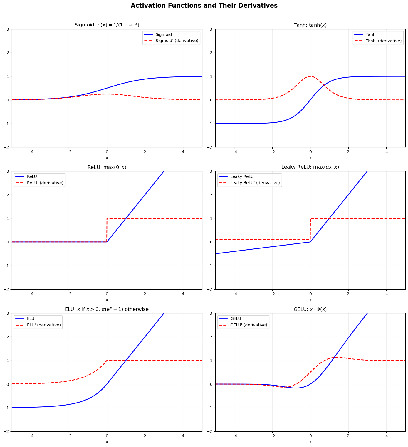
This means the derivative can be computed directly from the function value itself – no need to recompute \(e^{-x}\). The maximum value is \(\sigma'(0) = 1/4\), and the derivative approaches 0 in both tails.

Proof. Using the quotient rule:

\[\sigma'(x) = \frac{d}{dx}\left(\frac{1}{1+e^{-x}}\right) = \frac{e^{-x}}{(1+e^{-x})^2}\]

Now observe:

\[\sigma(x)(1-\sigma(x)) = \frac{1}{1+e^{-x}} \cdot \frac{e^{-x}}{1+e^{-x}} = \frac{e^{-x}}{(1+e^{-x})^2}\]

Therefore \(\sigma'(x) = \sigma(x)(1 - \sigma(x))\). \(\blacksquare\)

Maximum Derivative Value

The maximum of \(\sigma'(x)\) occurs at \(x = 0\):

\[\sigma'(0) = \sigma(0)(1-\sigma(0)) = \frac{1}{2} \cdot \frac{1}{2} = \frac{1}{4}\]

This bound of \(1/4\) is the root cause of the vanishing gradient problem.

17.2 The Hyperbolic Tangent (Tanh)

Definition

\[\tanh(x) = \frac{e^x - e^{-x}}{e^x + e^{-x}}\]

Relation to Sigmoid

\[\tanh(x) = 2\sigma(2x) - 1\]

Properties

• Range: \((-1, 1)\)

• Zero-centered: \(\tanh(0) = 0\) (unlike sigmoid, which has \(\sigma(0) = 0.5\))

• Odd function: \(\tanh(-x) = -\tanh(x)\)

• Saturates at both extremes

Theorem: Derivative of Tanh

\[\tanh'(x) = 1 - \tanh^2(x)\]

Proof. Let \(t = \tanh(x)\). Using the quotient rule with \(u = e^x - e^{-x}\), \(v = e^x + e^{-x}\):

\[\tanh'(x) = \frac{u'v - uv'}{v^2} = \frac{(e^x+e^{-x})(e^x+e^{-x}) - (e^x-e^{-x})(e^x-e^{-x})}{(e^x+e^{-x})^2}\]

\[= \frac{(e^x+e^{-x})^2 - (e^x-e^{-x})^2}{(e^x+e^{-x})^2} = 1 - \frac{(e^x-e^{-x})^2}{(e^x+e^{-x})^2} = 1 - \tanh^2(x) \qquad \blacksquare\]

Maximum: \(\tanh'(0) = 1 - 0 = 1\). Better than sigmoid’s \(1/4\), but still \(\leq 1\).

17.3 Rectified Linear Unit (ReLU)

Definition

\[\begin{split}\text{ReLU}(x) = \max(0, x) = \begin{cases} x & \text{if } x > 0 \\ 0 & \text{if } x \leq 0 \end{cases}\end{split}\]

Derivative

\[\begin{split}\text{ReLU}'(x) = \begin{cases} 1 & \text{if } x > 0 \\ 0 & \text{if } x < 0 \end{cases}\end{split}\]

(Technically undefined at \(x = 0\); in practice we set it to 0 or 1.)

Properties

• Range: \([0, \infty)\)

• Non-saturating for \(x > 0\): the gradient is exactly 1

• Computationally cheap: just a threshold comparison

• Sparse activation: outputs zero for half the input space

• Not differentiable at 0 (but this is a set of measure zero)

Tip

Why ReLU works – The constant gradient of 1 for positive inputs alleviates saturation-related vanishing gradients for active units, but does not prevent vanishing or exploding gradients in general. Unlike sigmoid (max derivative 0.25) and tanh (max derivative 1.0 but often much less), ReLU passes gradients through unchanged for active neurons. This simple property was the key insight that enabled training networks with dozens or hundreds of layers.

The Dying ReLU Problem

If a neuron’s pre-activation \(z\) is consistently negative (for all training examples), then \(\text{ReLU}'(z) = 0\) and the gradient is zero. The neuron receives no gradient signal and can never recover. It is effectively “dead.”

This can happen if:

• The learning rate is too large, causing a large negative bias

• Initialization places the neuron in a consistently negative regime

Warning

Dead ReLU neurons – If a ReLU neuron’s input is always negative, it outputs 0 forever and never recovers. This is an irreversible failure mode. In practice, dead neurons can affect 10-40% of all neurons in a network, especially with large learning rates or poor initialization. Solutions include Leaky ReLU (\(\alpha = 0.01\) for negative inputs), careful learning rate tuning, and proper initialization (He initialization).

17.4 Variants of ReLU

Leaky ReLU (Maas et al., 2013)

\[\begin{split}\text{LeakyReLU}(x) = \begin{cases} x & \text{if } x > 0 \\ \alpha x & \text{if } x \leq 0 \end{cases}\end{split}\]

where \(\alpha\) is a small constant (typically \(\alpha = 0.01\)). This prevents dying neurons.

Exponential Linear Unit (ELU, Clevert et al., 2015)

\[\begin{split}\text{ELU}(x) = \begin{cases} x & \text{if } x > 0 \\ \alpha(e^x - 1) & \text{if } x \leq 0 \end{cases}\end{split}\]

Smooth at \(x = 0\), with mean activations closer to zero.

Gaussian Error Linear Unit (GELU, Hendrycks & Gimpel, 2016)

\[\text{GELU}(x) = x \cdot \Phi(x)\]

where \(\Phi(x)\) is the CDF of the standard normal. Approximated by:

\[\text{GELU}(x) \approx 0.5x\left(1 + \tanh\left[\sqrt{2/\pi}(x + 0.044715x^3)\right]\right)\]

GELU is the default activation in BERT and GPT models.

Show code cell source Hide code cell source

import numpy as np
import matplotlib.pyplot as plt
from scipy.stats import norm

# Activation functions and their derivatives

x = np.linspace(-5, 5, 1000)

# Sigmoid
sigmoid = 1 / (1 + np.exp(-x))
sigmoid_deriv = sigmoid * (1 - sigmoid)

# Tanh
tanh = np.tanh(x)
tanh_deriv = 1 - tanh**2

# ReLU
relu = np.maximum(0, x)
relu_deriv = (x > 0).astype(float)

# Leaky ReLU
alpha_lrelu = 0.1
leaky_relu = np.where(x > 0, x, alpha_lrelu * x)
leaky_relu_deriv = np.where(x > 0, 1, alpha_lrelu)

# ELU
alpha_elu = 1.0
elu = np.where(x > 0, x, alpha_elu * (np.exp(x) - 1))
elu_deriv = np.where(x > 0, 1, alpha_elu * np.exp(x))

# GELU
gelu = x * norm.cdf(x)
gelu_deriv = norm.cdf(x) + x * norm.pdf(x)

# Plot all in a 3x2 grid
fig, axes = plt.subplots(3, 2, figsize=(14, 15))

activations = [
    (sigmoid, sigmoid_deriv, 'Sigmoid', r'$\sigma(x) = 1/(1+e^{-x})$'),
    (tanh, tanh_deriv, 'Tanh', r'$\tanh(x)$'),
    (relu, relu_deriv, 'ReLU', r'$\max(0, x)$'),
    (leaky_relu, leaky_relu_deriv, 'Leaky ReLU', r'$\max(\alpha x, x)$'),
    (elu, elu_deriv, 'ELU', r'$x$ if $x>0$, $\alpha(e^x-1)$ otherwise'),
    (gelu, gelu_deriv, 'GELU', r'$x \cdot \Phi(x)$'),
]

for idx, (f, df, name, formula) in enumerate(activations):
    row, col = divmod(idx, 2)
    ax = axes[row, col]
    ax.plot(x, f, 'b-', linewidth=2, label=f'{name}')
    ax.plot(x, df, 'r--', linewidth=2, label=f"{name}' (derivative)")
    ax.axhline(y=0, color='gray', linewidth=0.5)
    ax.axvline(x=0, color='gray', linewidth=0.5)
    ax.set_title(f'{name}: {formula}', fontsize=12)
    ax.legend(fontsize=10)
    ax.set_xlim(-5, 5)
    ax.set_ylim(-2, 3)
    ax.grid(True, alpha=0.2)
    ax.set_xlabel('x')

plt.suptitle('Activation Functions and Their Derivatives', fontsize=15, fontweight='bold', y=1.01)
plt.tight_layout()
plt.show()

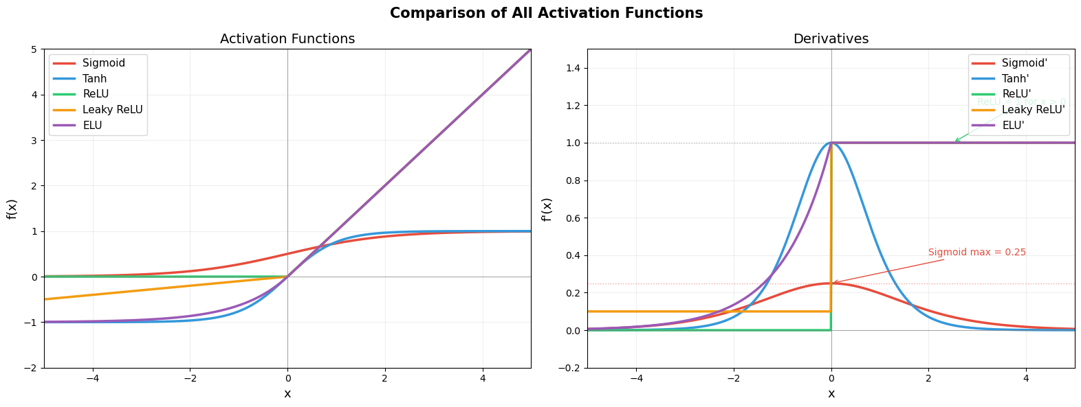
All Activation Functions on a Single Comparison Plot

The following visualization overlays all major activation functions and their derivatives on the same axes for direct comparison.

Show code cell source Hide code cell source

import numpy as np
import matplotlib.pyplot as plt
from scipy.stats import norm

x = np.linspace(-5, 5, 1000)

# Compute all activation functions
sig = 1 / (1 + np.exp(-x))
functions = {
    'Sigmoid': sig,
    'Tanh': np.tanh(x),
    'ReLU': np.maximum(0, x),
    'Leaky ReLU': np.where(x > 0, x, 0.1 * x),
    'ELU': np.where(x > 0, x, 1.0 * (np.exp(x) - 1)),
}

# Derivatives
derivatives = {
    'Sigmoid': sig * (1 - sig),
    'Tanh': 1 - np.tanh(x)**2,
    'ReLU': (x > 0).astype(float),
    'Leaky ReLU': np.where(x > 0, 1.0, 0.1),
    'ELU': np.where(x > 0, 1.0, np.exp(x)),
}

colors = ['#E74C3C', '#3498DB', '#2ECC71', '#F39C12', '#9B59B6']

fig, axes = plt.subplots(1, 2, figsize=(16, 6))

# Left: activation functions
for (name, f), color in zip(functions.items(), colors):
    axes[0].plot(x, f, color=color, linewidth=2.5, label=name)

axes[0].axhline(y=0, color='gray', linewidth=0.5)
axes[0].axvline(x=0, color='gray', linewidth=0.5)
axes[0].set_xlabel('x', fontsize=13)
axes[0].set_ylabel('f(x)', fontsize=13)
axes[0].set_title('Activation Functions', fontsize=14)
axes[0].legend(fontsize=11)
axes[0].set_xlim(-5, 5)
axes[0].set_ylim(-2, 5)
axes[0].grid(True, alpha=0.2)

# Right: derivatives
for (name, deriv), color in zip(derivatives.items(), colors):
    axes[1].plot(x, deriv, color=color, linewidth=2.5, label=f"{name}'")

axes[1].axhline(y=0, color='gray', linewidth=0.5)
axes[1].axhline(y=0.25, color='#E74C3C', linewidth=1, linestyle=':', alpha=0.5)
axes[1].axhline(y=1.0, color='gray', linewidth=1, linestyle=':', alpha=0.5)
axes[1].axvline(x=0, color='gray', linewidth=0.5)
axes[1].set_xlabel('x', fontsize=13)
axes[1].set_ylabel("f'(x)", fontsize=13)
axes[1].set_title('Derivatives', fontsize=14)
axes[1].legend(fontsize=11)
axes[1].set_xlim(-5, 5)
axes[1].set_ylim(-0.2, 1.5)
axes[1].grid(True, alpha=0.2)

# Annotate key values
axes[1].annotate('Sigmoid max = 0.25', xy=(0, 0.25), xytext=(2, 0.4),
                fontsize=10, color='#E74C3C',
                arrowprops=dict(arrowstyle='->', color='#E74C3C'))
axes[1].annotate('ReLU = 1 for x > 0', xy=(2.5, 1.0), xytext=(3, 1.2),
                fontsize=10, color='#2ECC71',
                arrowprops=dict(arrowstyle='->', color='#2ECC71'))

plt.suptitle('Comparison of All Activation Functions', fontsize=15, fontweight='bold')
plt.tight_layout()
plt.show()

17.5 The Vanishing Gradient Problem

The Core Issue

Recall the backpropagation equation (BP2):

\[\boldsymbol{\delta}^{(l)} = \left((\mathbf{W}^{(l+1)})^\top \boldsymbol{\delta}^{(l+1)}\right) \odot \sigma'^{(l)}(\mathbf{z}^{(l)})\]

Unrolling this recursion from the output layer \(L\) to layer \(l\):

\[\boldsymbol{\delta}^{(l)} = \left(\prod_{k=l}^{L-1} \text{diag}(\sigma'^{(k)}(\mathbf{z}^{(k)})) \, (\mathbf{W}^{(k+1)})^\top \right) \boldsymbol{\delta}^{(L)}\]

The gradient at layer \(l\) is a product of \((L - l)\) terms, each involving \(\sigma'\).

Danger

❗ Vanishing Gradient Problem – THE fundamental obstacle for deep networks. With sigmoid activation, gradients shrink by a factor of at most 0.25 at each layer. After 10 layers: \(0.25^{10} \approx 10^{-6}\). Gradients effectively disappear! Early layers receive essentially zero gradient signal and never learn meaningful features. This is why deep networks with sigmoid activation could not be trained before ~2010.

The Sigmoid Case

For sigmoid: \(\max_x \sigma'(x) = 1/4\).

After passing through \(k\) sigmoid layers, the gradient is attenuated by a factor of at most:

\[\left(\frac{1}{4}\right)^k\]

Layers \(k\)	Attenuation factor	Scientific notation
1	0.25	\(2.5 \times 10^{-1}\)
3	0.0156	\(1.6 \times 10^{-2}\)
5	\(9.77 \times 10^{-4}\)	\(\approx 10^{-3}\)
10	\(9.54 \times 10^{-7}\)	\(\approx 10^{-6}\)
20	\(9.09 \times 10^{-13}\)	\(\approx 10^{-12}\)

For \(k = 10\): the gradient is attenuated by a factor of approximately \(9.5 \times 10^{-7}\). This means early layers learn roughly a million times slower than the output layer.

Why This Kills Deep Learning

1. Early layers receive essentially zero gradient.

2. These layers never learn meaningful features.

3. Adding more layers makes things worse, not better.

4. This is why deep networks with sigmoid activation could not be trained before ~2010.

Show code cell source Hide code cell source

import numpy as np
import matplotlib.pyplot as plt

np.random.seed(42)

def create_network(layer_sizes, activation='sigmoid'):
    """Create a network with given layer sizes and activation."""
    params = []
    for i in range(len(layer_sizes) - 1):
        n_in, n_out = layer_sizes[i], layer_sizes[i+1]
        # Xavier initialization
        W = np.random.randn(n_out, n_in) * np.sqrt(2.0 / (n_in + n_out))
        b = np.zeros((n_out, 1))
        params.append((W, b))
    return params

def forward_pass(x, params, activation='sigmoid'):
    """Forward pass, returning all z's and a's."""
    a = x
    cache = [{'a': a}]
    for W, b in params:
        z = W @ a + b
        if activation == 'sigmoid':
            a = 1 / (1 + np.exp(-np.clip(z, -500, 500)))
        elif activation == 'relu':
            a = np.maximum(0, z)
        cache.append({'z': z, 'a': a})
    return a, cache

def backward_pass(y, params, cache, activation='sigmoid'):
    """Backward pass, returning gradient norms per layer."""
    L = len(params)
    a_out = cache[-1]['a']
    
    # MSE loss gradient
    dL_da = a_out - y
    
    # Output layer delta
    z = cache[-1]['z']
    if activation == 'sigmoid':
        sig = 1 / (1 + np.exp(-np.clip(z, -500, 500)))
        sigma_prime = sig * (1 - sig)
    elif activation == 'relu':
        sigma_prime = (z > 0).astype(float)
    
    delta = dL_da * sigma_prime
    
    grad_norms = [np.linalg.norm(delta)]
    
    # Backpropagate
    for l in range(L - 1, 0, -1):
        W = params[l][0]
        z = cache[l]['z']
        
        if activation == 'sigmoid':
            sig = 1 / (1 + np.exp(-np.clip(z, -500, 500)))
            sigma_prime = sig * (1 - sig)
        elif activation == 'relu':
            sigma_prime = (z > 0).astype(float)
        
        delta = (W.T @ delta) * sigma_prime
        grad_norms.append(np.linalg.norm(delta))
    
    grad_norms.reverse()  # layer 1 to L
    return grad_norms

# Experiment: gradient norms for different depths
depths = [3, 5, 10, 20]
n_features = 10
hidden_size = 20

# Generate a random input
x = np.random.randn(n_features, 1)
y = np.random.randn(1, 1)

fig, axes = plt.subplots(1, 2, figsize=(16, 6))

# === SIGMOID ===
for depth in depths:
    sizes = [n_features] + [hidden_size] * depth + [1]
    params = create_network(sizes, 'sigmoid')
    a_out, cache = forward_pass(x, params, 'sigmoid')
    grad_norms = backward_pass(y, params, cache, 'sigmoid')
    
    layers = list(range(1, len(grad_norms) + 1))
    axes[0].plot(layers, grad_norms, 'o-', label=f'{depth} hidden layers', linewidth=2, markersize=5)

axes[0].set_xlabel('Layer (from input to output)', fontsize=12)
axes[0].set_ylabel('Gradient Norm', fontsize=12)
axes[0].set_title('Sigmoid: Gradient Vanishes in Deep Networks', fontsize=13)
axes[0].set_yscale('log')
axes[0].legend(fontsize=10)
axes[0].grid(True, alpha=0.3)

# === ReLU ===
for depth in depths:
    sizes = [n_features] + [hidden_size] * depth + [1]
    params = create_network(sizes, 'relu')
    a_out, cache = forward_pass(x, params, 'relu')
    grad_norms = backward_pass(y, params, cache, 'relu')
    
    layers = list(range(1, len(grad_norms) + 1))
    axes[1].plot(layers, grad_norms, 'o-', label=f'{depth} hidden layers', linewidth=2, markersize=5)

axes[1].set_xlabel('Layer (from input to output)', fontsize=12)
axes[1].set_ylabel('Gradient Norm', fontsize=12)
axes[1].set_title('ReLU: Gradients Flow Through Deep Networks', fontsize=13)
axes[1].set_yscale('log')
axes[1].legend(fontsize=10)
axes[1].grid(True, alpha=0.3)

plt.suptitle('The Vanishing Gradient Problem: Sigmoid vs ReLU', fontsize=15, fontweight='bold')
plt.tight_layout()
plt.show()

print("Sigmoid: gradients decay exponentially with depth.")
print("ReLU: gradients maintain their magnitude across layers.")

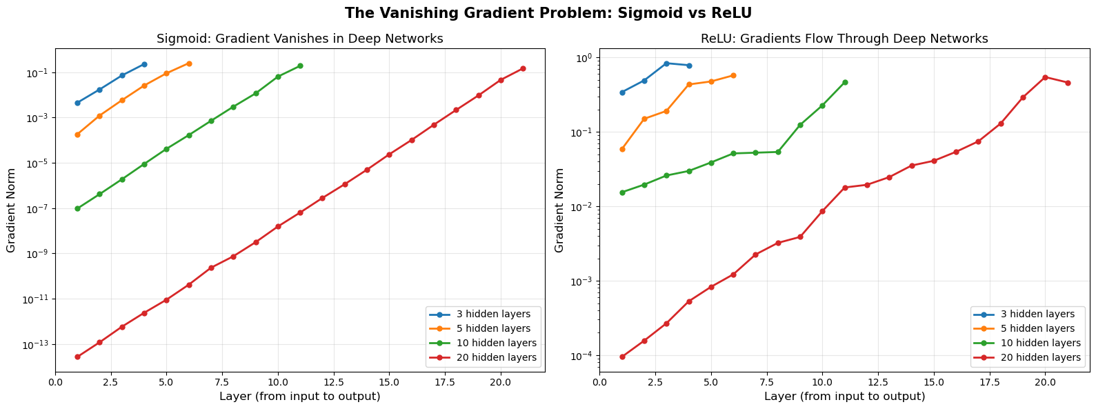
Sigmoid: gradients decay exponentially with depth.
ReLU: gradients maintain their magnitude across layers.

Vanishing Gradient Demonstration: Sigmoid vs ReLU Across 10 Layers

The following dramatic visualization shows the gradient magnitude at each layer of a 10-layer network for both sigmoid and ReLU activations.

Show code cell source Hide code cell source

import numpy as np
import matplotlib.pyplot as plt

np.random.seed(42)

# Build a 10-hidden-layer network and track gradient magnitudes
n_layers = 10
n_features = 8
hidden_size = 15
layer_sizes = [n_features] + [hidden_size] * n_layers + [1]

def run_experiment(activation):
    """Run forward/backward pass and return gradient norms per layer."""
    np.random.seed(42)
    # Initialize weights
    weights = []
    for i in range(len(layer_sizes) - 1):
        n_in, n_out = layer_sizes[i], layer_sizes[i+1]
        W = np.random.randn(n_out, n_in) * np.sqrt(2.0 / (n_in + n_out))
        weights.append(W)
    
    # Forward pass
    x = np.random.randn(n_features, 1)
    a_list = [x]
    z_list = []
    a = x
    
    for W in weights:
        z = W @ a
        if activation == 'sigmoid':
            a = 1 / (1 + np.exp(-np.clip(z, -500, 500)))
        else:
            a = np.maximum(0, z)
        z_list.append(z)
        a_list.append(a)
    
    # Backward pass
    y = np.random.randn(1, 1)
    dL_da = a_list[-1] - y
    
    if activation == 'sigmoid':
        s = 1 / (1 + np.exp(-np.clip(z_list[-1], -500, 500)))
        sp = s * (1 - s)
    else:
        sp = (z_list[-1] > 0).astype(float)
    
    delta = dL_da * sp
    grad_norms = [float(np.linalg.norm(delta))]
    
    for l in range(len(weights) - 1, 0, -1):
        if activation == 'sigmoid':
            s = 1 / (1 + np.exp(-np.clip(z_list[l-1], -500, 500)))
            sp = s * (1 - s)
        else:
            sp = (z_list[l-1] > 0).astype(float)
        delta = (weights[l].T @ delta) * sp
        grad_norms.append(float(np.linalg.norm(delta)))
    
    grad_norms.reverse()
    return grad_norms

# Run experiments
sigmoid_grads = run_experiment('sigmoid')
relu_grads = run_experiment('relu')

# Create visualization
fig, axes = plt.subplots(1, 2, figsize=(16, 7))

layers = range(1, len(sigmoid_grads) + 1)

# Sigmoid: bar chart showing vanishing
norm_sig = np.array(sigmoid_grads, dtype=float)
# Clamp tiny values for display
norm_sig = np.maximum(norm_sig, 1e-30)
colors_sig = plt.cm.Reds(np.linspace(0.3, 0.9, len(norm_sig)))
bars1 = axes[0].bar(layers, norm_sig, color=colors_sig, edgecolor='black', linewidth=0.5)
axes[0].set_xlabel('Layer (1 = closest to input)', fontsize=13)
axes[0].set_ylabel('Gradient Norm', fontsize=13)
axes[0].set_title('Sigmoid: Gradients VANISH', fontsize=14, color='red', fontweight='bold')
axes[0].set_yscale('log')
axes[0].grid(True, alpha=0.3, axis='y')

# ReLU: bar chart showing gradient preservation
norm_relu = np.array(relu_grads, dtype=float)
norm_relu = np.maximum(norm_relu, 1e-30)
colors_relu = plt.cm.Greens(np.linspace(0.3, 0.9, len(norm_relu)))
bars2 = axes[1].bar(layers, norm_relu, color=colors_relu, edgecolor='black', linewidth=0.5)
axes[1].set_xlabel('Layer (1 = closest to input)', fontsize=13)
axes[1].set_ylabel('Gradient Norm', fontsize=13)
axes[1].set_title('ReLU: Gradients FLOW', fontsize=14, color='green', fontweight='bold')
axes[1].set_yscale('log')
axes[1].grid(True, alpha=0.3, axis='y')

plt.suptitle(f'Gradient Magnitude Across {n_layers} Hidden Layers',
             fontsize=14, fontweight='bold')
plt.tight_layout()
plt.show()

print(f"Sigmoid: gradient at layer 1 is {sigmoid_grads[0]:.2e}, at layer {n_layers+1} is {sigmoid_grads[-1]:.2e}")
print(f"ReLU:    gradient at layer 1 is {relu_grads[0]:.2e}, at layer {n_layers+1} is {relu_grads[-1]:.2e}")
if sigmoid_grads[-1] > 0:
    print(f"Sigmoid ratio (layer 1 / layer {n_layers+1}): {sigmoid_grads[0]/sigmoid_grads[-1]:.1e}")

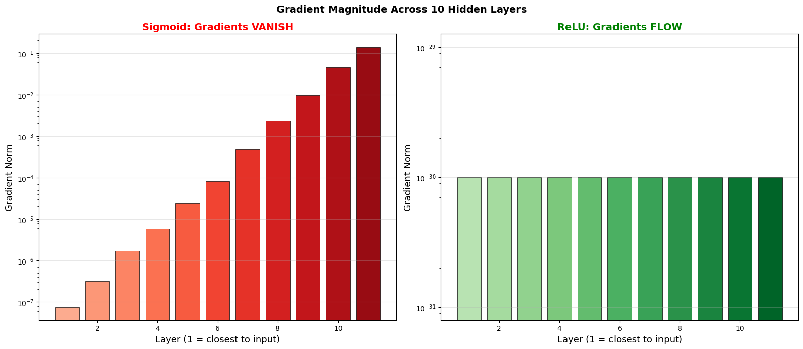
Sigmoid: gradient at layer 1 is 7.57e-08, at layer 11 is 1.40e-01
ReLU:    gradient at layer 1 is 0.00e+00, at layer 11 is 0.00e+00
Sigmoid ratio (layer 1 / layer 11): 5.4e-07

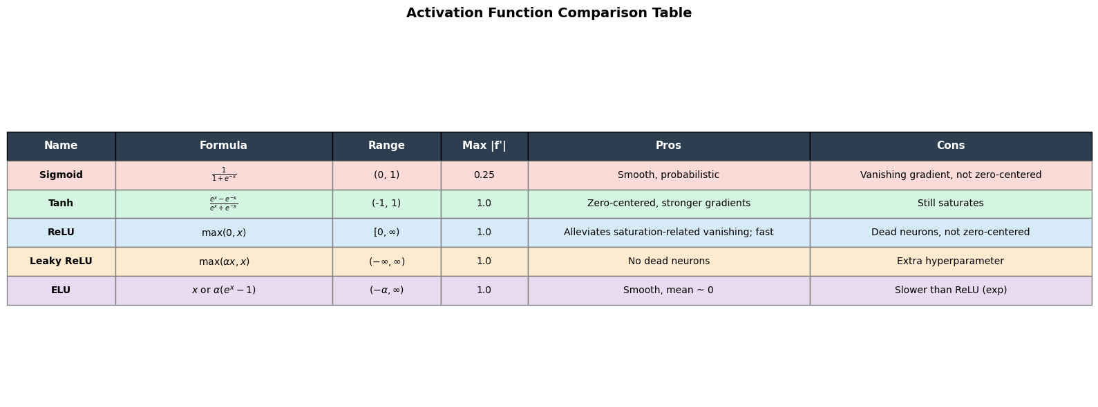
Activation Function Comparison Table

The following table summarizes the key properties, advantages, and disadvantages of each activation function.

Show code cell source Hide code cell source

import matplotlib.pyplot as plt
import numpy as np

fig, ax = plt.subplots(figsize=(16, 6))
ax.axis('off')

# Table data
columns = ['Name', 'Formula', 'Range', 'Max |f\'|', 'Pros', 'Cons']
rows = [
    ['Sigmoid', r'$\frac{1}{1+e^{-x}}$', '(0, 1)', '0.25',
     'Smooth, probabilistic', 'Vanishing gradient, not zero-centered'],
    ['Tanh', r'$\frac{e^x - e^{-x}}{e^x + e^{-x}}$', '(-1, 1)', '1.0',
     'Zero-centered, stronger gradients', 'Still saturates'],
    ['ReLU', r'$\max(0, x)$', r'$[0, \infty)$', '1.0',
     'Alleviates saturation-related vanishing; fast', 'Dead neurons, not zero-centered'],
    ['Leaky ReLU', r'$\max(\alpha x, x)$', r'$(-\infty, \infty)$', '1.0',
     'No dead neurons', 'Extra hyperparameter'],
    ['ELU', r'$x$ or $\alpha(e^x-1)$', r'$(-\alpha, \infty)$', '1.0',
     'Smooth, mean ~ 0', 'Slower than ReLU (exp)'],
]

# Row colors
row_colors = ['#FADBD8', '#D5F5E3', '#D6EAF8', '#FDEBD0', '#E8DAEF']
header_color = '#2C3E50'

table = ax.table(
    cellText=rows,
    colLabels=columns,
    loc='center',
    cellLoc='center',
    colWidths=[0.10, 0.20, 0.10, 0.08, 0.26, 0.26]
)

table.auto_set_font_size(False)
table.set_fontsize(10)
table.scale(1, 2.2)

# Style header
for j in range(len(columns)):
    cell = table[0, j]
    cell.set_facecolor(header_color)
    cell.set_text_props(color='white', fontweight='bold', fontsize=11)

# Style data rows
for i in range(len(rows)):
    for j in range(len(columns)):
        cell = table[i + 1, j]
        cell.set_facecolor(row_colors[i])
        cell.set_edgecolor('gray')
        if j == 0:  # Name column bold
            cell.set_text_props(fontweight='bold')

ax.set_title('Activation Function Comparison Table', fontsize=14, fontweight='bold', pad=20)

plt.tight_layout()
plt.savefig('activation_table.png', dpi=150, bbox_inches='tight')
plt.show()

17.6 Solutions to the Vanishing Gradient Problem

1. ReLU Activation

As demonstrated above, ReLU has a derivative of exactly 1 for positive inputs, preventing gradient decay. This was a key breakthrough that enabled training of deeper networks (Glorot, Bordes & Bengio, 2011; Krizhevsky, Sutskever & Hinton, 2012).

2. Residual Connections (He et al., 2015)

Instead of \(\mathbf{a}^{(l)} = \sigma(\mathbf{z}^{(l)})\), use:

\[\mathbf{a}^{(l)} = \sigma(\mathbf{z}^{(l)}) + \mathbf{a}^{(l-1)}\]

The identity shortcut allows gradients to flow directly through the addition, bypassing the nonlinearity. This enabled training of networks with 100+ layers.

3. Batch Normalization (Ioffe & Szegedy, 2015)

Normalize the pre-activations to have zero mean and unit variance within each mini-batch. This keeps the activations in the non-saturating regime of sigmoid/tanh.

4. Careful Initialization

Xavier initialization (Glorot & Bengio, 2010) for sigmoid/tanh:

\[W_{ij} \sim \mathcal{N}\left(0, \frac{2}{n_{\text{in}} + n_{\text{out}}}\right)\]

He initialization (He et al., 2015) for ReLU:

\[W_{ij} \sim \mathcal{N}\left(0, \frac{2}{n_{\text{in}}}\right)\]

These initialization schemes are designed to maintain the variance of activations and gradients across layers.

17.7 The Historical Arc: From Step to Sigmoid to ReLU

Era	Activation	Why	Limitation
1943	Step function	McCulloch-Pitts: binary logic	Not differentiable
1958	Step function	Rosenblatt’s perceptron	Cannot use gradient descent
1986	Sigmoid	Smooth, differentiable, bounded	Vanishing gradient
~1990s	Tanh	Zero-centered (better than sigmoid)	Still saturates
~2011	ReLU	Non-saturating, fast to compute	Dying ReLU
~2015+	Leaky ReLU, ELU	Fix dying ReLU	Minor improvements
~2016+	GELU, SiLU/Swish	Smooth ReLU alternatives	Used in transformers

The progression shows a recurring pattern: each activation solved a problem but introduced new ones, driving the search for better alternatives.

Exercises

Exercise 17.1. Prove that the sigmoid function is the unique solution to the differential equation \(f'(x) = f(x)(1 - f(x))\) with \(f(0) = 1/2\).

Exercise 17.2. Show that \(\tanh(x) = 2\sigma(2x) - 1\). Using this, derive \(\tanh'(x)\) from \(\sigma'(x)\).

Exercise 17.3. Implement Leaky ReLU and ELU. Create the same gradient norm experiment as in Section 17.5 and compare Sigmoid, Tanh, ReLU, Leaky ReLU, and ELU.

Exercise 17.4. For a 10-layer network with tanh activation, compute the theoretical maximum gradient attenuation factor (using \(\max|\tanh'| = 1\)). Why is tanh better than sigmoid for gradient flow, even though both saturate?

Exercise 17.5. Implement Xavier and He initialization. For networks with 10, 20, and 50 hidden layers, plot the distribution of activations in each layer for (a) standard normal initialization, (b) Xavier initialization, © He initialization. Which maintains the activation variance best?