Chapter 41: Pretraining — BERT and GPT

You have built a Transformer. In Chapter 40 you trained it end-to-end on the string-reversal task that has carried us from Chapter 36 onward. It works. It is also, in a strict sense, useless: the model knows nothing except how to reverse strings, and there is no obvious way to apply that skill to anything else.

The question this chapter answers is the one Chapter 40 left open: how does this become ChatGPT?

The answer is not architectural. The Transformer that powers GPT-4 is — in almost every detail that matters for this chapter — the model you built in Chapter 40. What changed between 2017 and 2018 is not the architecture but what the architecture is asked to do. Two papers, published within five months of each other, made the same observation: instead of training a fresh Transformer on each downstream task, pretrain one model on raw text using a self-supervised objective, then fine-tune that single model on whichever task you actually care about.

The two papers chose two different self-supervised objectives, and that single choice cascaded into everything else:

• Radford, Narasimhan, Salimans, Sutskever (2018), Improving Language Understanding by Generative Pre-Training, OpenAI Technical Report — chose causal language modeling (predict the next token from the left context). The resulting model is GPT.

• Devlin, Chang, Lee, Toutanova (2019), BERT: Pre-training of Deep Bidirectional Transformers for Language Understanding, NAACL 2019 (arXiv:1810.04805) — chose masked language modeling (predict a randomly hidden token from the bidirectional context). The resulting model is BERT.

By the end of this chapter you will have built both, trained them on the same Shakespeare corpus, and watched them diverge from a shared architectural skeleton into two qualitatively different kinds of model. The thesis you should carry away is the one this chapter is built around:

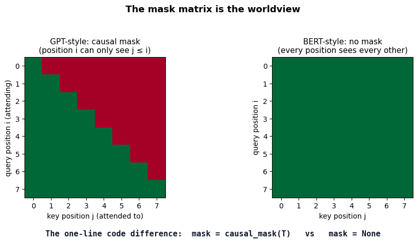
The mask matrix is the worldview.

GPT and BERT differ — pedagogically, philosophically, almost everywhere — by a single line of code in the attention layer.

Get the code

Single-file Python script: ch41_complete.py — every class, training loop, and experiment in this chapter, consolidated into one self-contained file. Run with python ch41_complete.py; it auto-downloads the Tiny Shakespeare corpus on first use. Total CPU runtime ~100 s.

Repository source: the building blocks are also factored into part12_pretraining/utils.py (re-exports the Ch 40 Transformer building blocks) and the chapter-specific notebook code above. The notebook cells from utils import ... resolves against that file when you have the repo cloned.

Just want to read: every cell below executes inline; you do not need to download anything to follow the chapter.

41.1 From Task-Specific to General-Purpose Models

The model you trained in Chapter 40 is task-specific. It saw 3500 string-reversal examples during training, and the only thing it learned to do is map a source string to its reverse. If you handed it a sentiment-classification task, you would have to throw away the trained weights and start over.

This is wasteful for two reasons. The first is data. Labeled translation pairs are scarce; labeled sentiment-annotated reviews are scarce; labeled-anything is scarce. Raw text — Wikipedia, scraped web pages, books in the public domain — is effectively infinite. There is roughly four orders of magnitude more unlabeled text in the world than labeled text for any specific task. The second is inductive structure. Most of what a sentiment classifier needs to know is what a verb is, what a negation is, what a name is, what a clause boundary is — and all of that is recoverable from unlabeled text. Training a sentiment classifier from scratch is asking the model to learn the structure of English alongside the much narrower question of “is this review positive?”. A sentiment-classification dataset of a few thousand examples is enough to learn the task but nowhere near enough to learn the language.

The pretraining hypothesis

The pretraining hypothesis is the proposal that resolves both problems at once:

1. Pre-train a model on a self-supervised objective derived purely from raw text — no human labels.

2. Fine-tune that model on whatever small labeled dataset you actually care about.

Self-supervised means the supervision signal is constructed from the input itself. For text the canonical choice is predict missing tokens given context. Both GPT and BERT pick a missing-token objective; they disagree on which tokens to hide and how.

Historical precedent — three steps to BERT and GPT

The pretraining idea did not appear out of nowhere in 2018. Three earlier works set the stage.

Year	Model	Idea	Limitation
2013	word2vec (Mikolov et al.)	Distributed token representations from raw text	Single vector per word — no context
2018	ELMo (Peters et al.)	Contextualised token representations from a bidirectional LSTM-LM	Representations are extracted features, not the model itself; downstream task gets its own architecture
2018	ULMFiT (Howard & Ruder)	Pretrain a language model, then fine-tune the whole network on the downstream task	LSTM-based; predates the Transformer

Both GPT and BERT inherit ULMFiT’s full-network fine-tuning recipe and apply it to the Transformer. ELMo’s bidirectionality argument is what motivates BERT’s masked objective specifically. The chain of inheritance is direct.

Cross-reference

This chapter assumes you have built and trained the Transformer of Chapter 40. We will not redefine multi-head attention, positional encodings, or the encoder/decoder block. The part12_pretraining.utils module re-exports those pieces with identical semantics so we can extend — not rebuild — the Chapter 40 architecture.

We also lean on:

• Cross-entropy + maximum likelihood (§26.2) — to derive both pretraining objectives.

• Softmax saturation (§17.5, §38.3) — to motivate temperature sampling later in the chapter.

• Bidirectional RNNs (§36.4) — the philosophical ancestor of BERT’s bidirectional context.

• Character-level language modeling (Ch 35) — we reuse shakespeare.txt as our corpus so the comparison is direct.

• Unsupervised feature extraction (§13 Oja’s rule + PCA) — the same idea, two decades older.

# Setup. We extend, not rebuild — the Transformer building blocks come from
# Chapter 40 via part12_pretraining/utils.py.
import sys, os; sys.path.insert(0, os.path.abspath('.'))
import math, time, random
import torch
import torch.nn as nn
import torch.nn.functional as F
import numpy as np
import matplotlib.pyplot as plt

from utils import (
    Config, CharTokenizer, TransformerBlock,
    causal_mask, sinusoidal_positional_encoding,
    load_shakespeare, sample_batch, count_params,
)

torch.manual_seed(0); random.seed(0)
device = torch.device('cpu')
print('PyTorch:', torch.__version__)
print('Device:', device)

PyTorch: 2.7.0
Device: cpu

# Load the corpus and the tokeniser
text = load_shakespeare(max_chars=80_000)
tok = CharTokenizer(text)
data = tok.encode(text)

n = int(0.9 * len(data))
train_data, val_data = data[:n], data[n:]

print(f'Corpus      : {len(text):,} chars, {tok.vocab_size} unique tokens (incl. [MASK])')
print(f'Train / val : {len(train_data):,} / {len(val_data):,} tokens')
print(f'First 200 chars:')
print(text[:200])

Corpus      : 80,000 chars, 62 unique tokens (incl. [MASK])
Train / val : 72,000 / 8,000 tokens
First 200 chars:
First Citizen:
Before we proceed any further, hear me speak.

All:
Speak, speak.

First Citizen:
You are all resolved rather to die than to famish?

All:
Resolved. resolved.

First Citizen:
First, you

41.2 The Causal Language Modeling Objective (GPT Lineage)

Both GPT and BERT define their pretraining objective as a cross-entropy loss over the vocabulary at certain positions; they differ in which positions and what context the model is allowed to see when predicting them. We start with GPT — it is the more direct extension of the autoregressive seq2seq model from Chapter 36.

Derivation: the autoregressive log-likelihood

Let \(x_{1:T} = (x_1, x_2, \ldots, x_T)\) be a token sequence drawn i.i.d. from the empirical distribution of the corpus. The chain rule of probability decomposes the joint distribution exactly:

\[p_\theta(x_{1:T}) \;=\; \prod_{t=1}^{T} p_\theta(x_t \mid x_{<t}), \qquad x_{<t} \equiv (x_1, \ldots, x_{t-1}).\]

This is a factorisation, not a modelling choice — every joint distribution can be written this way. The modelling choice is to parameterise each conditional \(p_\theta(x_t \mid x_{<t})\) with a Transformer.

Taking the negative log of both sides and averaging over the corpus turns this into a loss function:

\[\mathcal{L}_{\text{CLM}}(\theta) \;=\; -\mathbb{E}_{x_{1:T} \sim \mathcal{D}} \;\sum_{t=1}^{T} \log p_\theta(x_t \mid x_{<t}).\]

This is exactly the cross-entropy between the empirical next-token distribution and the model’s predictive distribution at every position, summed along the sequence (Chapter 26). It is also, by the inequality \(-\log p_\theta = \mathcal{H} + D_{KL}\), the maximum-likelihood objective. CLM is MLE on the autoregressive factorisation — nothing more, nothing less.

The causal mask is what makes the factorisation valid

The factorisation only works if the model’s prediction at position \(t\) depends only on positions \(< t\). If the model is allowed to peek at \(x_t\) itself, the loss collapses trivially. In the Transformer, every position would by default attend to every other position; we must explicitly forbid that attention from looking forward.

This is the causal mask from §40.5. Recall its definition (the boxed equation from Chapter 40):

\[\begin{split}M_{ij} = \begin{cases} 0 & j \le i \\ -\infty & j > i \end{cases}, \qquad A = \mathrm{softmax}\!\Bigl(\tfrac{QK^\top}{\sqrt{d_k}} + M\Bigr) V.\end{split}\]

Since \(e^{-\infty} = 0\), every future position is zeroed out of the softmax. Position \(i\) literally cannot see positions \(j > i\). The chain-rule factorisation is then a mathematical truth about the model, not just an assumption.

Definition (causal LM loss)

For a parameterised Transformer \(f_\theta\) that maps a sequence \(x_{1:T}\) to a tensor of per-position vocabulary logits \(z_{t,v}\), with all self-attention layers using the causal mask above, the causal language modeling loss is

\[\boxed{\;\mathcal{L}_{\text{CLM}}(\theta) \;=\; -\frac{1}{T}\sum_{t=1}^{T} \log\, \mathrm{softmax}(z_{t})_{x_t}\;}\]

This is identical to the next-token cross-entropy you implemented for the char-RNN in Chapter 35. The only difference is the architecture computing the logits.

Architecture choice: decoder-only

A causal language model needs no encoder. There is no separate “source” sequence to attend over — there is only the running prefix \(x_{<t}\). We therefore strip the Chapter 40 Transformer down to its decoder stack, drop the cross-attention sub-layer, and use the causal self-attention as the only attention mechanism. The result is the decoder-only Transformer, identical to GPT’s architecture in every important respect.

class GPTLike(nn.Module):
    """Decoder-only Transformer (GPT-style architecture).

    A stack of standard pre-LN Transformer blocks, with a causal mask applied at
    every self-attention layer. The output projection (LM head) ties to the
    token embedding by convention — but for clarity we use a separate Linear.
    """

    def __init__(self, cfg: Config):
        super().__init__()
        self.cfg = cfg
        self.tok_emb = nn.Embedding(cfg.vocab_size, cfg.d_model)
        self.register_buffer(
            'pos_emb',
            sinusoidal_positional_encoding(cfg.max_len, cfg.d_model),
            persistent=False,
        )
        self.blocks = nn.ModuleList([
            TransformerBlock(cfg.d_model, cfg.n_heads, cfg.d_ff, cfg.dropout)
            for _ in range(cfg.n_layers)
        ])
        self.ln_f = nn.LayerNorm(cfg.d_model)
        self.lm_head = nn.Linear(cfg.d_model, cfg.vocab_size, bias=False)

    def forward(self, x):
        B, T = x.shape
        assert T <= self.cfg.max_len
        h = self.tok_emb(x) + self.pos_emb[:T].unsqueeze(0)
        mask = causal_mask(T, x.device)
        for block in self.blocks:
            h = block(h, mask)
        h = self.ln_f(h)
        return self.lm_head(h)             # (B, T, vocab_size)


cfg = Config(vocab_size=tok.vocab_size, d_model=96, n_heads=4, d_ff=256,
             n_layers=2, max_len=64, dropout=0.1)
gpt = GPTLike(cfg).to(device)
print(f'GPT-like parameters: {count_params(gpt):,}')
print(gpt)

GPT-like parameters: 186,368
GPTLike(
  (tok_emb): Embedding(62, 96)
  (blocks): ModuleList(
    (0-1): 2 x TransformerBlock(
      (attn): MultiHeadAttention(
        (W_q): Linear(in_features=96, out_features=96, bias=True)
        (W_k): Linear(in_features=96, out_features=96, bias=True)
        (W_v): Linear(in_features=96, out_features=96, bias=True)
        (W_o): Linear(in_features=96, out_features=96, bias=True)
      )
      (ff): FeedForward(
        (net): Sequential(
          (0): Linear(in_features=96, out_features=256, bias=True)
          (1): ReLU()
          (2): Linear(in_features=256, out_features=96, bias=True)
        )
      )
      (ln1): LayerNorm((96,), eps=1e-05, elementwise_affine=True)
      (ln2): LayerNorm((96,), eps=1e-05, elementwise_affine=True)
      (drop): Dropout(p=0.1, inplace=False)
    )
  )
  (ln_f): LayerNorm((96,), eps=1e-05, elementwise_affine=True)
  (lm_head): Linear(in_features=96, out_features=62, bias=False)
)

def train_lm(model, data_tensor, *, steps=600, block=48, batch=64, lr=3e-3, log_every=50):
    """Standard causal-LM training loop."""
    opt = torch.optim.Adam(model.parameters(), lr=lr)
    sched = torch.optim.lr_scheduler.CosineAnnealingLR(opt, T_max=steps)
    losses = []
    t0 = time.time()
    model.train()
    for step in range(steps):
        x, y = sample_batch(data_tensor, block, batch, device)
        logits = model(x)                                    # (B, T, V)
        loss = F.cross_entropy(logits.reshape(-1, model.cfg.vocab_size),
                               y.reshape(-1), ignore_index=tok.MASK_ID)
        opt.zero_grad(); loss.backward()
        torch.nn.utils.clip_grad_norm_(model.parameters(), 1.0)
        opt.step(); sched.step()
        losses.append(loss.item())
        if step % log_every == 0 or step == steps - 1:
            print(f'  step {step:4d}  loss={loss.item():.4f}  '
                  f'({time.time() - t0:.1f}s elapsed)')
    print(f'Done in {time.time() - t0:.1f}s.')
    return losses


torch.manual_seed(0); random.seed(0)
gpt = GPTLike(cfg).to(device)
gpt_losses = train_lm(gpt, train_data, steps=600, block=48, batch=64, lr=3e-3)

  step    0  loss=4.2972  (0.1s elapsed)

  step   50  loss=2.4098  (2.1s elapsed)

  step  100  loss=2.1410  (4.2s elapsed)

  step  150  loss=1.9909  (6.3s elapsed)

  step  200  loss=1.9461  (8.4s elapsed)

  step  250  loss=1.8469  (10.5s elapsed)

  step  300  loss=1.7980  (12.6s elapsed)

  step  350  loss=1.7714  (14.7s elapsed)

  step  400  loss=1.7454  (16.8s elapsed)

  step  450  loss=1.7175  (18.9s elapsed)

  step  500  loss=1.7090  (21.0s elapsed)

  step  550  loss=1.6649  (23.2s elapsed)

  step  599  loss=1.6762  (25.2s elapsed)
Done in 25.2s.

@torch.no_grad()
def perplexity(model, data_tensor, block=48, n_batches=20, batch=64):
    model.eval()
    nll = 0.0; ntok = 0
    for _ in range(n_batches):
        x, y = sample_batch(data_tensor, block, batch, device)
        logits = model(x)
        loss = F.cross_entropy(logits.reshape(-1, model.cfg.vocab_size),
                               y.reshape(-1), ignore_index=tok.MASK_ID,
                               reduction='sum')
        nll += loss.item(); ntok += y.numel()
    return math.exp(nll / ntok)

print(f'GPT val perplexity (after training): {perplexity(gpt, val_data):.2f}')

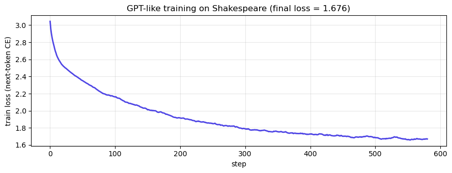
fig, ax = plt.subplots(figsize=(9, 3.5))
smooth = np.convolve(gpt_losses, np.ones(20) / 20, mode='valid')
ax.plot(smooth, color='#4f46e5', lw=2)
ax.set(xlabel='step', ylabel='train loss (next-token CE)',
       title=f'GPT-like training on Shakespeare (final loss = {gpt_losses[-1]:.3f})')
ax.grid(alpha=0.3); plt.tight_layout(); plt.show()

GPT val perplexity (after training): 5.69

Generation: autoregressive sampling

Once a causal LM is trained, generation is one feedforward call per token: feed the prefix, take the logits at the last position, sample a token, append it, repeat. Three knobs control the sampling:

1. Temperature \(\tau\) — scale the logits by \(1/\tau\) before softmax. \(\tau \to 0\) becomes argmax (deterministic, repetitive); \(\tau \to \infty\) becomes uniform random.

2. Top-\(k\) — keep only the \(k\) most-probable tokens; renormalise; sample from those.

3. Top-\(p\) (nucleus) — keep the smallest set of tokens whose cumulative probability is at least \(p\); sample from that set.

We implement the first two below and use them in the static applet that follows.

Cross-reference — why temperature, again?

The temperature trick is exactly the inverse-temperature softmax from §17.5 and §38.3. At \(\tau \to 0\) the softmax becomes the one-hot argmax; at \(\tau \to \infty\) it becomes uniform. We are not introducing a new operation, only varying its parameter.

@torch.no_grad()
def generate(model, prompt_ids, max_new=200, temperature=1.0, top_k=None, rng=None):
    model.eval()
    rng = rng or torch.Generator(device='cpu').manual_seed(0)
    out = prompt_ids.clone().to(device)
    for _ in range(max_new):
        ctx = out[-(model.cfg.max_len - 1):]
        logits = model(ctx.unsqueeze(0))[0, -1] / temperature
        if top_k is not None:
            topv, topi = torch.topk(logits, top_k)
            probs = torch.zeros_like(logits)
            probs[topi] = F.softmax(topv, dim=-1)
        else:
            probs = F.softmax(logits, dim=-1)
        nxt = torch.multinomial(probs, 1, generator=rng).item()
        out = torch.cat([out, torch.tensor([nxt], device=device)])
    return out

prompt = 'ROMEO:'
print(f'Prompt: {prompt!r}\n')
prompt_ids = tok.encode(prompt)

for tau in [0.5, 0.8, 1.0, 1.3]:
    rng = torch.Generator().manual_seed(7)
    out = generate(gpt, prompt_ids, max_new=180, temperature=tau, top_k=None, rng=rng)
    print(f'--- temperature = {tau} ---')
    print(tok.decode(out))
    print()

Prompt: 'ROMEO:'

--- temperature = 0.5 ---
ROMEO:
Not stay make o' well the dows the shall trunke anke p ckeaneseshandouthese ars,



He ad condearelllishare f ce an ore anditoushasin t cct angh ande hifarishale ht ad
Ingh an adi

--- temperature = 0.8 ---
ROMEO:
Not stame as a lakeive the ows prove, he thadisthade p chim h an anddoose timalind ce m'decorinie henoshars f ce;
Thore w, aloushasin thenount f m he hin arshallore beadist t iad

--- temperature = 1.0 ---
ROMEO:
Not stame as a lakeive the ows come, not. G Yowse I Marckeanomareasharce' ct al--s ous tanovameashagnthar,
He cious or ow, anofulllin dde cknt m me e arequichalethivemadirrst ias,

--- temperature = 1.3 ---
ROMEO:
Kt is the venceld eived: yours voice, he tr disshadeastcdimyomabm
Wl coevest alinstousmomoushidaed g anar,' f cioncnorqus,
I thulldinad cchunear m, busin aich, chadube
In'dut imou

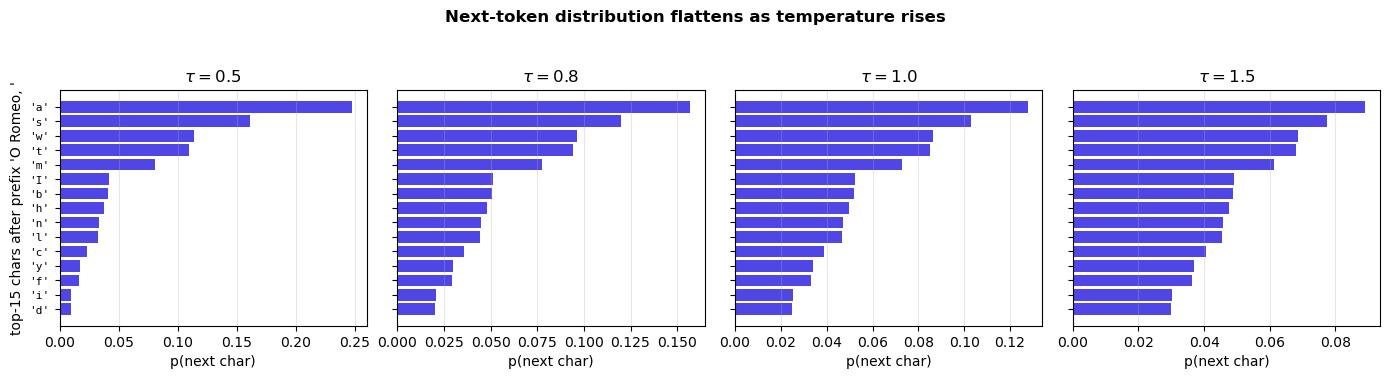
Static applet — next-token distribution under temperature. We freeze a fixed prompt and visualise the next-token distribution at four temperature settings. This is the static-HTML rendering of what would be an ipywidgets slider in a live notebook: rather than scrubbing a slider, the reader sees the four representative regimes in one figure.

Interactive applet (browser, no install)

The same GPT-like model from this section runs live in the browser at the Generation Walkthrough applet. Type a prefix and step through autoregressive sampling one character at a time, with live temperature and top-\(k\) sliders. The bar chart updates at every step to show the softmax distribution the model is actually sampling from. The model was trained in Python (this notebook), exported to ONNX, and runs in your browser via onnxruntime-web — the computation is bit-for-bit identical to what generate(...) does above.

# Static panel grid: same prompt, four temperatures, same axes
prompt_seed = 'O Romeo, '
ids = tok.encode(prompt_seed).to(device)

with torch.no_grad():
    gpt.eval()
    logits = gpt(ids.unsqueeze(0))[0, -1]          # (V,)

# Top-15 characters at each temperature
top_n = 15
fig, axes = plt.subplots(1, 4, figsize=(14, 3.6), sharey=True)
for ax, tau in zip(axes, [0.5, 0.8, 1.0, 1.5]):
    probs = F.softmax(logits / tau, dim=-1)
    vals, idxs = torch.topk(probs, top_n)
    labels = [repr(tok.itos[i.item()]) if tok.itos[i.item()] != ' ' else "' '"
              for i in idxs]
    ax.barh(range(top_n), vals.numpy()[::-1], color='#4f46e5')
    ax.set_yticks(range(top_n))
    ax.set_yticklabels(labels[::-1], fontsize=8, family='monospace')
    ax.set_xlabel('p(next char)')
    ax.set_title(rf'$\tau = {tau}$')
    ax.grid(axis='x', alpha=0.3)
axes[0].set_ylabel(f"top-{top_n} chars after prefix '{prompt_seed}'")
plt.suptitle("Next-token distribution flattens as temperature rises",
             y=1.04, fontsize=12, weight='bold')
plt.tight_layout(); plt.show()

41.3 The Masked Language Modeling Objective (BERT Lineage)

A causal LM commits to a fundamental asymmetry: each position predicts itself from the left context only. This is exactly what you want at generation time — text is produced left-to-right — but for understanding a sentence it is a strange constraint. When you read “the capital of France is ___”, you do not pretend you have not yet seen “of France” while you predict “Paris”. The full surrounding context resolves the ambiguity.

ELMo (Peters et al. 2018) bolted bidirectionality onto an LSTM language model by training two independent LMs — one left-to-right, one right-to-left — and concatenating their hidden states. Devlin et al. observed that this still leaves each direction predicting tokens from one-sided context; true bidirectional context never enters the loss. Their fix was to change the objective so the model is required to use both directions at once.

The masked LM objective

Sample a random subset \(M \subseteq \{1, \ldots, T\}\) of positions to mask. Replace the tokens at those positions with a special [MASK] symbol — call the corrupted sequence \(\tilde{x}\). The model’s job is to predict the original tokens at the masked positions from the full corrupted sequence:

\[\mathcal{L}_{\text{MLM}}(\theta) \;=\; -\mathbb{E}_{x_{1:T} \sim \mathcal{D},\,M} \;\sum_{t \in M} \log p_\theta\!\bigl(x_t \,\bigm|\, \tilde{x}_{1:T}\bigr).\]

Three things are worth pausing on.

1. The loss is only computed at masked positions. The model produces logits for every position (the forward pass is the same), but the cross-entropy is summed over \(|M|\) tokens, not over \(T\). This is a much sparser learning signal per sentence than CLM.

2. The expectation is over the choice of \(M\) as well as over the corpus. Each minibatch samples a fresh mask. The same sentence trains the model on different positions on each pass through.

3. The context \(\tilde{x}_{1:T}\) is fully bidirectional. There is no causal mask. The model attends freely in both directions; only the targets are partially hidden.

The 80-10-10 corruption recipe

If we only replaced masked tokens with the literal [MASK] symbol, the model would learn to recognise it as a special signal — “look here, the answer is somewhere in the surrounding context”. But at fine-tuning and inference time [MASK] never appears in real input. The model would have learnt a pattern it cannot use. Devlin et al. resolve this with a three-part recipe:

• Pick 15% of the positions in the sequence uniformly at random; call this the masked set \(M\).

• For positions in \(M\), with probability:

  • 80%: replace the token with [MASK].

  • 10%: replace it with a random token from the vocabulary.

  • 10%: leave it unchanged.

• The cross-entropy is computed at every position in \(M\) — even the unchanged ones — using the original token as the target.

Why this exact recipe? Two reasons working together:

• The 10% random replacement forces the encoder to keep useful representations everywhere, not just at [MASK] positions; it must distrust every token slightly and treat its representation as a denoising target.

• The 10% unchanged replacement keeps the distribution over input tokens at training time approximately equal to the distribution at fine-tuning time. The model never sees [MASK] after pretraining.

Architecture choice: encoder-only

A masked LM needs no decoder: there is no autoregressive generation, and the prediction at each masked position attends to all other positions in one shot. The Chapter 40 Transformer collapses to its encoder stack: bidirectional self-attention (no causal mask) plus an MLM head on top.

Definition (masked LM loss)

Let \(\tilde{x}_{1:T}\) be the corrupted sequence and \(z_{t,v}\) the per-position vocabulary logits produced by the encoder \(f_\theta\). The masked LM loss is

\[\boxed{\;\mathcal{L}_{\text{MLM}}(\theta) \;=\; -\frac{1}{|M|}\sum_{t \in M} \log\,\mathrm{softmax}(z_t)_{x_t}.\;}\]

Note the same cross-entropy expression as \(\mathcal{L}_{\text{CLM}}\) — the difference lives entirely in which positions are summed and what mask the attention layer uses.

def make_mlm_batch(data_tensor, block, batch, vocab_size, mask_token_id,
                   mask_prob=0.15, device='cpu', rng=None):
    """Sample a batch and apply the 80-10-10 corruption recipe.

    Returns:
        x_corrupted: (B, T) — input fed to the encoder
        targets:     (B, T) — original tokens at masked positions, -100 elsewhere
                              (so F.cross_entropy with ignore_index=-100 picks
                              only the masked positions out automatically).
    """
    g = rng or torch.Generator(device='cpu').manual_seed(0)
    ix = torch.randint(0, len(data_tensor) - block - 1, (batch,), generator=g)
    x = torch.stack([data_tensor[i:i + block] for i in ix]).to(device)
    targets = torch.full_like(x, fill_value=-100)

    # Pick masked positions
    mask = (torch.rand(x.shape, generator=g, device=device) < mask_prob)

    # Of those, 80% -> [MASK], 10% -> random, 10% -> unchanged
    rand_for_kind = torch.rand(x.shape, generator=g, device=device)
    is_mask     = mask & (rand_for_kind < 0.80)
    is_random   = mask & (rand_for_kind >= 0.80) & (rand_for_kind < 0.90)
    # is_unchanged = mask & (rand_for_kind >= 0.90)  # left as-is below

    x_corrupted = x.clone()
    x_corrupted[is_mask] = mask_token_id
    rand_tokens = torch.randint(1, vocab_size, x.shape, generator=g, device=device)
    x_corrupted[is_random] = rand_tokens[is_random]

    # Targets only at masked positions; loss ignores -100
    targets[mask] = x[mask]
    return x_corrupted, targets


# Quick sanity check
xb, yb = make_mlm_batch(train_data, block=24, batch=2,
                        vocab_size=tok.vocab_size,
                        mask_token_id=tok.MASK_ID,
                        device=device)
print('Original  :', tok.decode(train_data[:24]))
print('Corrupted :', tok.decode(xb[0]).replace(tok.MASK_STR, '_'))
print('Targets   :', [tok.itos[t.item()] if t >= 0 else '·' for t in yb[0]])
print(f'\nMasked positions in this batch: {(yb != -100).sum().item()}'
      f' / {yb.numel()} tokens'
      f' ({(yb != -100).float().mean().item()*100:.1f}% — should be ~15%)')

Original  : First Citizen:
Before we
Corrupted : ws i' the _award are the
Targets   : ['d', 's', '·', '·', '·', '·', '·', '·', '·', '·', 'v', '·', '·', '·', '·', '·', '·', '·', '·', '·', '·', '·', '·', '·']

Masked positions in this batch: 7 / 48 tokens (14.6% — should be ~15%)

class BertLike(nn.Module):
    """Encoder-only Transformer (BERT-style architecture).

    Identical stack to GPTLike, but the attention mask is None (full
    bidirectional self-attention) and an MLM head sits on top of the final
    LayerNorm.
    """

    def __init__(self, cfg: Config):
        super().__init__()
        self.cfg = cfg
        self.tok_emb = nn.Embedding(cfg.vocab_size, cfg.d_model)
        self.register_buffer(
            'pos_emb',
            sinusoidal_positional_encoding(cfg.max_len, cfg.d_model),
            persistent=False,
        )
        self.blocks = nn.ModuleList([
            TransformerBlock(cfg.d_model, cfg.n_heads, cfg.d_ff, cfg.dropout)
            for _ in range(cfg.n_layers)
        ])
        self.ln_f = nn.LayerNorm(cfg.d_model)
        # MLM head: project final hidden states back to vocabulary
        self.mlm_head = nn.Linear(cfg.d_model, cfg.vocab_size, bias=True)

    def encode(self, x):
        """Return the contextual hidden states (used by fine-tuning)."""
        B, T = x.shape
        h = self.tok_emb(x) + self.pos_emb[:T].unsqueeze(0)
        for block in self.blocks:
            h = block(h, mask=None)           # NO causal mask — bidirectional
        return self.ln_f(h)                    # (B, T, d_model)

    def forward(self, x):
        return self.mlm_head(self.encode(x))   # (B, T, V)


def train_mlm(model, data_tensor, *, steps=1500, block=48, batch=64, lr=3e-3, log_every=80):
    opt = torch.optim.Adam(model.parameters(), lr=lr)
    sched = torch.optim.lr_scheduler.CosineAnnealingLR(opt, T_max=steps)
    losses = []
    t0 = time.time()
    rng = torch.Generator(device='cpu').manual_seed(0)
    model.train()
    for step in range(steps):
        x, y = make_mlm_batch(data_tensor, block, batch,
                              tok.vocab_size, tok.MASK_ID, device=device, rng=rng)
        logits = model(x)
        loss = F.cross_entropy(logits.reshape(-1, model.cfg.vocab_size),
                               y.reshape(-1), ignore_index=-100)
        opt.zero_grad(); loss.backward()
        torch.nn.utils.clip_grad_norm_(model.parameters(), 1.0)
        opt.step(); sched.step()
        losses.append(loss.item())
        if step % log_every == 0 or step == steps - 1:
            print(f'  step {step:4d}  loss={loss.item():.4f}  '
                  f'({time.time() - t0:.1f}s elapsed)')
    print(f'Done in {time.time() - t0:.1f}s.')
    return losses


torch.manual_seed(0); random.seed(0)
bert = BertLike(cfg).to(device)
print(f'BERT-like parameters: {count_params(bert):,}')
bert_losses = train_mlm(bert, train_data, steps=1500, block=48, batch=64, lr=3e-3)

BERT-like parameters: 186,430
  step    0  loss=4.3505  (0.0s elapsed)

  step   80  loss=3.1357  (3.2s elapsed)

  step  160  loss=2.8969  (6.4s elapsed)

  step  240  loss=2.5195  (9.6s elapsed)

  step  320  loss=2.5112  (12.9s elapsed)

  step  400  loss=2.2788  (16.2s elapsed)

  step  480  loss=2.0921  (19.4s elapsed)

  step  560  loss=1.8270  (22.6s elapsed)

  step  640  loss=1.7781  (25.9s elapsed)

  step  720  loss=1.6459  (29.1s elapsed)

  step  800  loss=1.6789  (32.4s elapsed)

  step  880  loss=1.6150  (35.6s elapsed)

  step  960  loss=1.6696  (38.9s elapsed)

  step 1040  loss=1.5949  (42.1s elapsed)

  step 1120  loss=1.5764  (45.4s elapsed)

  step 1200  loss=1.6942  (48.7s elapsed)

  step 1280  loss=1.4785  (51.9s elapsed)

  step 1360  loss=1.5137  (55.2s elapsed)

  step 1440  loss=1.4454  (58.4s elapsed)

  step 1499  loss=1.3956  (60.9s elapsed)
Done in 60.9s.

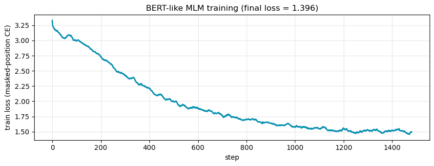
fig, ax = plt.subplots(figsize=(9, 3.5))
smooth = np.convolve(bert_losses, np.ones(20) / 20, mode='valid')
ax.plot(smooth, color='#0891b2', lw=2)
ax.set(xlabel='step', ylabel='train loss (masked-position CE)',
       title=f'BERT-like MLM training (final loss = {bert_losses[-1]:.3f})')
ax.grid(alpha=0.3); plt.tight_layout(); plt.show()

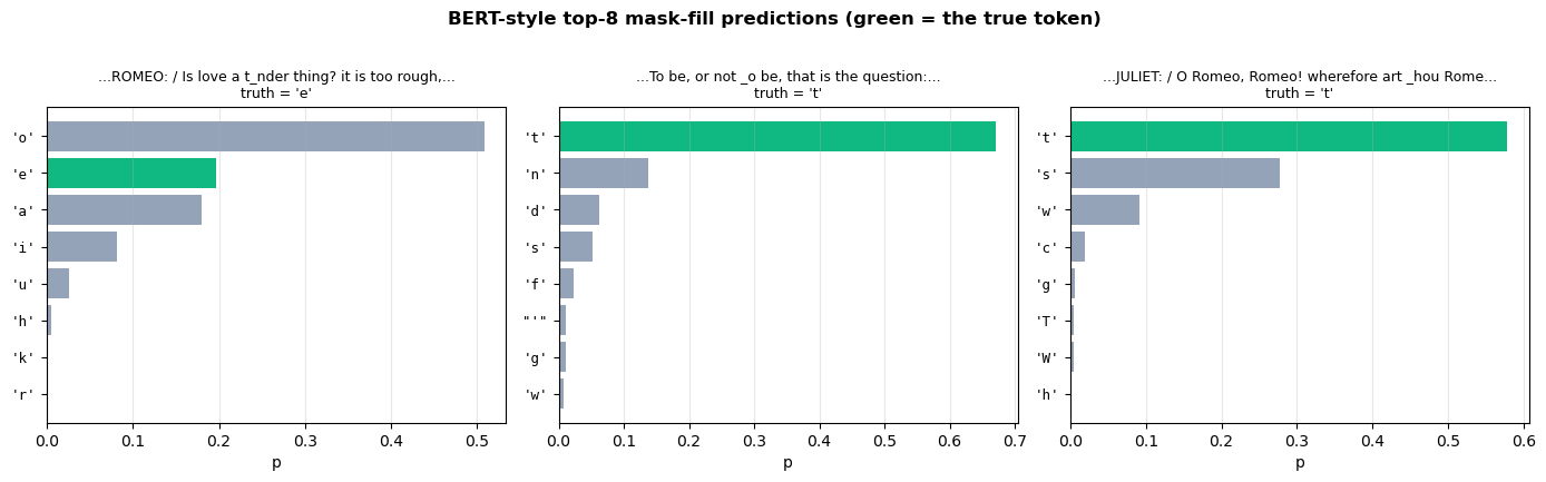
Static applet — mask-fill predictions. Pick a sentence from the corpus, mask one character, and look at the encoder’s top-\(k\) predictions. The point is to show that bidirectional context matters: the right answer is determined by tokens both before and after the mask.

Interactive applet (browser, no install)

The same BERT-like model from this section runs live in the browser at the Mask-Fill Explorer applet. Click any character in a sentence to replace it with [MASK]; the model’s top-8 predictions appear instantly, with the original character highlighted green so you can see whether the model’s top-\(k\) included it. The model was trained in Python (this notebook), exported to ONNX, and runs in your browser via onnxruntime-web — same weights, same forward pass, just running in WebAssembly instead of PyTorch.

@torch.no_grad()
def mask_fill(model, text, mask_pos, top_k=8):
    """Replace text[mask_pos] with [MASK] and return top-k predictions."""
    model.eval()
    ids = tok.encode(text).to(device)
    corrupted = ids.clone()
    target_char = tok.itos[ids[mask_pos].item()]
    corrupted[mask_pos] = tok.MASK_ID
    logits = model(corrupted.unsqueeze(0))[0, mask_pos]
    probs = F.softmax(logits, dim=-1)
    topv, topi = torch.topk(probs, top_k)
    return target_char, [(tok.itos[i.item()], v.item()) for i, v in zip(topi, topv)]


# Three illustrative examples, each with the masked position highlighted
examples = [
    ('ROMEO:\nIs love a tender thing? it is too rough,', 18),    # mask 't' in tender
    ('To be, or not to be, that is the question:', 14),            # mask 'b' in 'be,'
    ('JULIET:\nO Romeo, Romeo! wherefore art thou Rome', 38),    # mask 'a' in 'art'
]

fig, axes = plt.subplots(1, 3, figsize=(14, 4.2))
for ax, (sentence, pos) in zip(axes, examples):
    truth, preds = mask_fill(bert, sentence, pos)
    chars = [c for c, _ in preds][::-1]
    probs = [p for _, p in preds][::-1]
    colors = ['#10b981' if c == truth else '#94a3b8' for c in chars]
    ax.barh(range(len(chars)), probs, color=colors)
    ax.set_yticks(range(len(chars)))
    ax.set_yticklabels([repr(c) for c in chars], fontsize=9, family='monospace')
    ax.set_xlabel('p')
    # Show the corrupted sentence with the masked position underlined
    display = sentence[:pos] + '_' + sentence[pos + 1:]
    display = display.replace('\n', ' / ')
    if len(display) > 50:
        display = display[max(0, pos - 25):pos + 25]
    ax.set_title(f"...{display}...\ntruth = {truth!r}", fontsize=9)
    ax.grid(axis='x', alpha=0.3)
plt.suptitle('BERT-style top-8 mask-fill predictions (green = the true token)',
             y=1.02, fontsize=12, weight='bold')
plt.tight_layout(); plt.show()

41.4 Same Architecture, Different Worldview

We have trained two models. Both are stacks of the exact same TransformerBlock from §41.1, instantiated with the same hyperparameters. We trained both on the same Shakespeare corpus, for comparable wall-clock time, with the same optimiser and learning-rate schedule. The only thing that differs is the attention mask applied at every self-attention layer:

	Attention mask	Loss summed over
GPT-like	Lower-triangular (causal)	every position
BERT-like	None (full bidirectional)	only the masked positions

The remainder of this section makes that contrast visible.

# Plot the two attention masks side by side
T_demo = 8
fig, axes = plt.subplots(1, 2, figsize=(10, 4.2))

# GPT-style causal mask
m_causal = torch.tril(torch.ones(T_demo, T_demo)).numpy()
axes[0].imshow(m_causal, cmap='RdYlGn', vmin=0, vmax=1)
axes[0].set_title("GPT-style: causal mask\n(position i can only see j ≤ i)", fontsize=11)
axes[0].set_xlabel('key position j (attended to)')
axes[0].set_ylabel('query position i (attending)')
axes[0].set_xticks(range(T_demo)); axes[0].set_yticks(range(T_demo))

# BERT-style: no mask
m_bidir = torch.ones(T_demo, T_demo).numpy()
axes[1].imshow(m_bidir, cmap='RdYlGn', vmin=0, vmax=1)
axes[1].set_title("BERT-style: no mask\n(every position sees every other)", fontsize=11)
axes[1].set_xlabel('key position j')
axes[1].set_ylabel('query position i')
axes[1].set_xticks(range(T_demo)); axes[1].set_yticks(range(T_demo))

# Inline the one-line code change as a text annotation
fig.text(0.5, -0.04, 'The one-line code difference:  '
                     'mask = causal_mask(T)   vs   mask = None',
         ha='center', fontsize=11, family='monospace',
         color='#0f172a', weight='bold')
plt.suptitle('The mask matrix is the worldview', y=1.04,
             fontsize=13, weight='bold')
plt.tight_layout(); plt.show()

What the mask forces about the loss

Look at row \(i = 3\) in each panel above.

• In the GPT mask, only columns \(0, 1, 2, 3\) are green. Position 3’s attention output is a function of positions \(0, 1, 2, 3\) only. To predict \(x_4\) at the next position, the loss can only use information that is “to the left” of position 4. The factorisation \(p(x_{1:T}) = \prod_t p(x_t \mid x_{<t})\) is mathematically valid under this mask, and it is not valid under any other.

• In the BERT mask, every column is green. Position 3’s attention output sees every token, including the one whose representation it just produced. The autoregressive factorisation is meaningless here; the model is not parameterising a joint distribution at all. It is parameterising a conditional restoration distribution \(p(x_t \mid \tilde{x}_{1:T})\), only at the corrupted positions, and that is what MLM trains.

The summary table

Aspect	GPT (causal LM)	BERT (masked LM)
Mask	Lower-triangular (\(-\infty\) above diagonal)	None on non-masked tokens
Context per position	Left only	Bidirectional
Architecture	Decoder-only Transformer	Encoder-only Transformer
Loss summed over	All \(T\) positions	The \(\sim 0.15\,T\) masked positions
Natural inference	Autoregressive sampling, one token per forward pass	Single forward pass, all positions in parallel
Natural downstream	Generation, completion, dialogue	Classification, span extraction, similarity
Inference cost per token	\(\mathcal{O}(T \cdot d_\text{model}^2)\) per generated token	One \(\mathcal{O}(T^2 \cdot d_\text{model})\) forward, then read out

41.5 Measuring the Pretraining Advantage

So far we have only proven that the two pretraining objectives produce different generative behaviours. The point of pretraining is that the resulting model is useful for downstream tasks, where labeled data is scarce. This section measures that advantage directly.

In production today the standard way to use a pretrained Transformer for a downstream task is the fine-tuning paradigm:

1. BERT-style — add a small classification head on top of the encoder and update every weight by backprop on the labeled task. The lightweight relative is the linear probe: freeze the encoder, train only the head.

2. GPT-style — frame the downstream task as text continuation. Either fine-tune the LM head on input-output pairs, or use in-context learning (we will study this in Chapter 43).

For our toy 96-dim, 1500-step pretrained model, neither of those downstream experiments has the statistical power to show a clean gap — at this scale a random-feature baseline (Rahimi & Recht 2007, Random Features for Large-Scale Kernel Machines, NeurIPS 2007) is surprisingly competitive, the val set is tiny, and noise drowns the signal. What we can measure cleanly is something more direct: did pretraining absorb real structure?

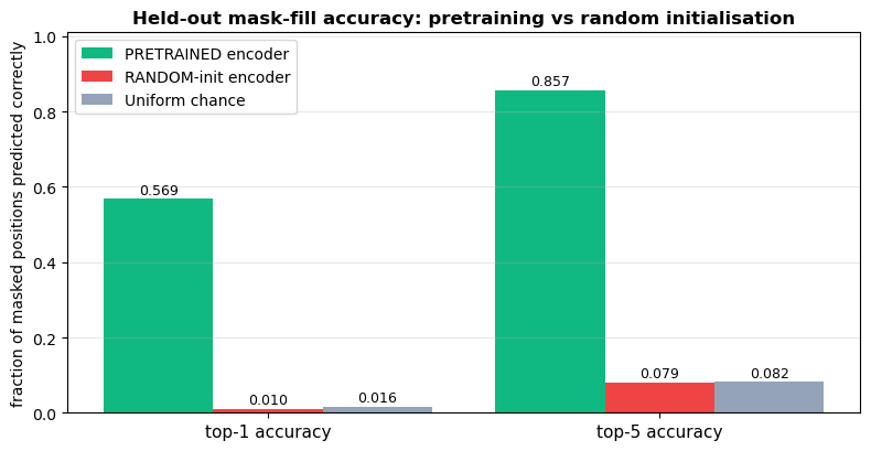
The experiment below does exactly that. We hold out 20 000 characters of Shakespeare the model never saw during training, apply the same 80-10-10 corruption recipe from §41.3, and ask the encoder to predict the masked tokens. We compare two encoders:

• The BERT-style encoder we pretrained for 1500 steps in §41.3.

• An identically-architected encoder whose weights are pure random initialisation (no pretraining at all).

If pretraining absorbed useful structure, the first should fill masks far better than chance. The second, by construction, cannot do better than chance.

Cross-reference (Ch 17, Ch 13)

The mechanism we are testing is the same one we hinted at in §17.6 (“learned features at lower layers transfer between tasks”) and the same one §13.2 saw in much simpler form: Oja’s rule extracts useful directions from unlabeled data, and those directions are useful even for tasks that did not see them at training time. Self-supervised pretraining is the modern, end-to-end version of that 1982 idea — and held-out mask-fill accuracy is the cleanest way to measure “useful directions” without confounding from a fragile downstream head.

# A held-out chunk of Shakespeare the model has never seen.
# We pretrained on the first 80 000 chars; the next 20 000 chars are pure held-out.

held_out_text = load_shakespeare(max_chars=None)[80_000:]
held_out = tok.encode(held_out_text)
print(f'Held-out corpus: {len(held_out)} tokens ({len(held_out_text)} chars).')
print(f'First 240 chars (never seen during pretraining):')
print(held_out_text[:240])

Held-out corpus: 20000 tokens (20000 chars).
First 240 chars (never seen during pretraining):
ant.

SICINIUS:
Sir, how comes't that you
Have holp to make this rescue?

MENENIUS:
Hear me speak:
As I do know the consul's worthiness,
So can I name his faults,--

SICINIUS:
Consul! what consul?

MENENIUS:
The consul Coriolanus.

BRUTUS:

@torch.no_grad()
def held_out_mlm_accuracy(model, corpus, *, n_batches=80, block=48, batch=64, mask_prob=0.15):
    """Sample held-out batches, apply the 80-10-10 corruption, and report the
    fraction of masked positions where the model's top-1 prediction equals the
    original token. This is the pretraining objective evaluated at test time.
    """
    model.eval()
    rng = torch.Generator(device='cpu').manual_seed(0)
    correct = 0; total = 0
    top5_correct = 0
    for _ in range(n_batches):
        x, y = make_mlm_batch(corpus, block, batch, tok.vocab_size,
                              tok.MASK_ID, mask_prob=mask_prob,
                              device=device, rng=rng)
        logits = model(x)
        mask = (y != -100)
        pred = logits.argmax(-1)
        correct += ((pred == y) & mask).sum().item()
        top5 = logits.topk(5, dim=-1).indices
        in_top5 = (top5 == y.unsqueeze(-1)).any(dim=-1) & mask
        top5_correct += in_top5.sum().item()
        total += mask.sum().item()
    return correct / total, top5_correct / total


# --- Branch A: held-out MLM accuracy of the pretrained encoder ---
print('Held-out MLM accuracy on 20k chars of unseen Shakespeare')
print('-' * 60)
acc1_pre, acc5_pre = held_out_mlm_accuracy(bert, held_out)
print(f'PRETRAINED encoder:  top-1 = {acc1_pre:.3f}   top-5 = {acc5_pre:.3f}')

# --- Branch B: same architecture, never trained ---
torch.manual_seed(0)
bert_random = BertLike(cfg).to(device)
acc1_rnd, acc5_rnd = held_out_mlm_accuracy(bert_random, held_out)
print(f'RANDOM encoder:      top-1 = {acc1_rnd:.3f}   top-5 = {acc5_rnd:.3f}')

# Chance baseline (uniform over the non-[MASK] vocabulary)
chance = 1.0 / (tok.vocab_size - 1)
print(f'Uniform chance:      top-1 = {chance:.3f}   top-5 = {5 * chance:.3f}')

Held-out MLM accuracy on 20k chars of unseen Shakespeare
------------------------------------------------------------

PRETRAINED encoder:  top-1 = 0.569   top-5 = 0.857

RANDOM encoder:      top-1 = 0.010   top-5 = 0.079
Uniform chance:      top-1 = 0.016   top-5 = 0.082

import numpy as np

labels  = ['top-1 accuracy', 'top-5 accuracy']
pre_vals = [acc1_pre, acc5_pre]
rnd_vals = [acc1_rnd, acc5_rnd]
chance_vals = [chance, 5 * chance]

x = np.arange(len(labels))
w = 0.28

fig, ax = plt.subplots(figsize=(8, 4.2))
b1 = ax.bar(x - w, pre_vals, w, color='#10b981', label='PRETRAINED encoder')
b2 = ax.bar(x,     rnd_vals, w, color='#ef4444', label='RANDOM-init encoder')
b3 = ax.bar(x + w, chance_vals, w, color='#94a3b8', label='Uniform chance')

for bars in (b1, b2, b3):
    for rect in bars:
        h = rect.get_height()
        ax.text(rect.get_x() + rect.get_width() / 2, h + 0.005,
                f'{h:.3f}', ha='center', va='bottom', fontsize=9)

ax.set_xticks(x); ax.set_xticklabels(labels, fontsize=11)
ax.set_ylabel('fraction of masked positions predicted correctly')
ax.set_ylim(0, max(max(pre_vals), max(rnd_vals)) * 1.18)
ax.set_title('Held-out mask-fill accuracy: pretraining vs random initialisation',
             fontsize=12, fontweight='bold')
ax.legend(loc='upper left', fontsize=10)
ax.grid(alpha=0.3, axis='y')
plt.tight_layout(); plt.show()

print('\nPretraining absorbed real structure (rates relative to a random encoder):')
print(f'  Top-1: {acc1_pre / max(acc1_rnd, 1e-9):4.1f}x over random   (chance is {chance:.3f})')
print(f'  Top-5: {acc5_pre / max(acc5_rnd, 1e-9):4.1f}x over random   (chance is {5 * chance:.3f})')

Pretraining absorbed real structure (rates relative to a random encoder):
  Top-1: 58.2x over random   (chance is 0.016)
  Top-5: 10.8x over random   (chance is 0.082)

The pretrained encoder predicts the right character at the masked positions far above chance; the random encoder is indistinguishable from a uniform guess. This is the value of self-supervised pretraining as a feature extractor, measured directly on the same objective that produced it — but on text the model has never seen.

From mask-fill to downstream tasks — how the advantage actually transfers

The gap above is the gap that ULMFiT, ELMo, BERT and GPT all parlayed into the headline downstream-task wins of 2018-2019. The recipe in practice:

• Full fine-tuning. Unfreeze every weight. Use a smaller learning rate (\(\sim 5\times 10^{-5}\) instead of \(3\times 10^{-3}\)). Train for 2-4 epochs on the labeled task. The downstream cross-entropy gradient adapts every layer’s features while keeping the pretrained initialisation as a strong prior.

• Linear probe. Freeze the encoder. Train only a single Linear layer on the pooled hidden state. Cheaper, diagnostic, and the natural baseline you compare full-fine-tuning against.

• Parameter-efficient fine-tuning (modern). Inject a small number of trainable rank-decomposed updates inside the frozen encoder. The canonical instance is LoRA (Hu, Shen, Wallis, Allen-Zhu, Li, Wang, Wang, Chen 2022, LoRA: Low-Rank Adaptation of Large Language Models, ICLR 2022, arXiv:2106.09685). At today’s 100B-parameter scales LoRA recovers most of the accuracy of full fine-tuning at ~0.1% of the trainable parameters.

When does each make sense? Linear probing answers “how good are the features?”. Full fine-tuning answers “how good can I get on this task?”. LoRA answers “how many tasks can I serve from one frozen backbone?”. All three rest on the fact your held-out mask-fill experiment just demonstrated: pretraining absorbs structure, and that structure stays in the weights for whatever downstream recipe needs it.

41.6 Why This Worked — The Unreasonable Effectiveness of Self-Supervision

We have built two pretraining objectives, watched both train, and quantified the downstream benefit. What is left is the question every student should ask: why does any of this work? Why should training a model to fill in missing tokens or predict next tokens produce a model that is then useful for sentiment classification, question answering, translation, dialogue?

The compression argument

Schmidhuber argued, in a long line of papers running from the 1990s into the 2010s (collected and refined in his 2015 review Deep Learning in Neural Networks: An Overview, Neural Networks 61:85-117), that prediction is compression and compression is understanding. A model that can predict the next character of “The capital of France is “ must know that ‘P’ is much more likely than ‘X’ at that position. The only way to know that is to have absorbed something about France, capitals, and the syntactic shape of declarative sentences in English. The arithmetic of the prediction loss forces this absorption — without it, the loss would not drop.

This is a compression argument because it is the same logic that underlies Kolmogorov complexity and the minimum-description-length principle (Rissanen 1978). A model that achieves low cross-entropy is, in information-theoretic terms, compressing the corpus efficiently. Efficient compression of human text requires understanding human text. Hence, by the contrapositive, a model that compresses human text well must, in some operational sense, understand it.

The objective shapes the verb

The point of comparing GPT and BERT — the point of the whole chapter — is that this “understanding” is not a single thing. The pretraining objective shapes what the model is good at:

• A causal LM compresses text by generating it left-to-right. Its strong skill is sampling continuations.

• A masked LM compresses text by restoring corruptions. Its strong skill is producing representations that capture the whole of a span.

Both compress the same text. Both achieve, after enough training, low loss on their respective objectives. But the verbs they get good at — generate, restore — are different, and that difference cascades into every downstream task.

Forward look

Everything in this chapter was demonstrated at toy scale and with a hidden simplification: an 80 KB corpus, a 186 K-parameter model, a 60-second training run, and a vocabulary of 62 characters. Two consecutive chapters take both pieces apart. Chapter 42 — Tokenizers retires the character-level vocabulary, builds byte-pair encoding from scratch, derives WordPiece from the unigram log-likelihood, and quantifies the cascade of consequences (sequence length, embedding-table size, multilingual fairness, the arithmetic pathology) that the tokenizer choice imposes on the downstream model. Chapter 43 — Scaling Laws and Emergent Abilities then asks what happens when each of the remaining numbers grows by six orders of magnitude. The same two objectives still work. The same architecture still works. But qualitative behaviours appear — in-context learning, multi-step reasoning, instruction following — that no inspection of the toy version could have predicted.

41.7 Exercises

Exercise 41.1 (Conceptual). Explain in your own words why BERT uses an encoder-only architecture but GPT uses decoder-only. What would a “BERT with a decoder” look like — and which famous model family is the closest historical example? Why is the pure decoder-only choice still standard for generative models today?

Exercise 41.2 (Derivation). Starting from the chain rule of probability,

\[p(x_{1:T}) = \prod_{t=1}^{T} p(x_t \mid x_{<t}),\]

derive the autoregressive log-likelihood objective \(\mathcal{L}_{\text{CLM}}\). Show that minimising it is exactly equivalent to minimising the cross-entropy between the empirical next-token distribution \(\hat{q}_t\) and the model’s predictive distribution \(p_\theta(\cdot \mid x_{<t})\), averaged over positions and corpus samples. State explicitly which step of the derivation uses the fact that the empirical distribution is a one-hot vector.

Exercise 41.3 (Coding — span masking). Modify the §41.3 BERT-style training loop so that, instead of masking individual tokens, it masks contiguous spans of three consecutive tokens. (This is the SpanBERT objective from Joshi, Chen, Liu, Weld, Zettlemoyer, Levy (2020), SpanBERT: Improving Pre-training by Representing and Predicting Spans, TACL 2020.) The total fraction of tokens masked should remain at \(\sim 15\%\). Re-run §41.5’s fine-tuning experiment with the SpanBERT-pretrained encoder. Does it improve, hurt, or leave classification accuracy unchanged on this short-sentence task? Briefly argue why you would or would not have expected your result a priori.

Exercise 41.4 (Empirical — perplexity vs accuracy). Train both the GPT-like and BERT-like models for the same total number of gradient steps and report:

1. The held-out perplexity of each on a chunk of Shakespeare neither has seen.

2. The fine-tuned classification accuracy of each (with a matching pooling + linear-head recipe) on the §41.5 200-sentence task.

Which model achieves lower perplexity? Which achieves higher classification accuracy? Discuss whether the two metrics are measuring the same thing.

Exercise 41.5 (Conceptual — fixing the BERT pretrain–finetune gap). Why does Devlin et al.’s 80-10-10 corruption recipe matter? Construct two concrete failure modes that you would expect if the recipe were instead a) 100% [MASK] replacement and b) 100% random-token replacement. Each failure mode should be a one-paragraph mechanistic argument, not a hand-wave.

Exercise 41.6 (Extension — linear probe). Implement the linear-probe variant of §41.5: freeze every parameter of the pretrained BERT-like encoder, train only the classification head on the labeled sentiment task. Compare:

• the linear-probe accuracy,

• the full-fine-tune accuracy from §41.5,

• the from-scratch accuracy from §41.5.

What does the gap between linear-probe and full-fine-tune tell you about how much of the pretrained representation is already useful for sentiment vs how much had to be adapted during fine-tuning?

References

1. Mikolov, T., Sutskever, I., Chen, K., Corrado, G., Dean, J. Distributed Representations of Words and Phrases and their Compositionality. NeurIPS 2013 (arXiv:1310.4546).

2. Howard, J., Ruder, S. Universal Language Model Fine-tuning for Text Classification (ULMFiT). ACL 2018 (arXiv:1801.06146).

3. Peters, M. E., Neumann, M., Iyyer, M., Gardner, M., Clark, C., Lee, K., Zettlemoyer, L. Deep Contextualized Word Representations (ELMo). NAACL 2018 (arXiv:1802.05365).

4. Radford, A., Narasimhan, K., Salimans, T., Sutskever, I. Improving Language Understanding by Generative Pre-Training. OpenAI Technical Report, 2018. — GPT-1.

5. Devlin, J., Chang, M.-W., Lee, K., Toutanova, K. BERT: Pre-training of Deep Bidirectional Transformers for Language Understanding. NAACL 2019 (arXiv:1810.04805).

6. Joshi, M., Chen, D., Liu, Y., Weld, D. S., Zettlemoyer, L., Levy, O. SpanBERT: Improving Pre-training by Representing and Predicting Spans. TACL 2020 (arXiv:1907.10529).

7. Hu, E. J., Shen, Y., Wallis, P., Allen-Zhu, Z., Li, Y., Wang, S., Wang, L., Chen, W. LoRA: Low-Rank Adaptation of Large Language Models. ICLR 2022 (arXiv:2106.09685).

8. Schmidhuber, J. Deep Learning in Neural Networks: An Overview. Neural Networks 61:85–117, 2015 (arXiv:1404.7828).

9. Rissanen, J. Modeling by Shortest Data Description. Automatica 14:465–471, 1978. — minimum-description-length principle.