Chapter 12: Hebbian Learning Theory

Chapter 12: Hebbian Learning Theory#

12.1 Historical Context: Donald Hebb and the Birth of Synaptic Learning#

Donald Olding Hebb (1904–1985) was a Canadian neuropsychologist whose work laid the theoretical foundation for understanding how neural connections strengthen through experience. His magnum opus, The Organization of Behavior (1949), proposed a neurophysiological theory of learning that would profoundly influence both neuroscience and artificial intelligence.

Hebb was trained under Karl Lashley at Harvard and later worked with Wilder Penfield at the Montreal Neurological Institute. His clinical observations of patients with brain lesions, combined with his theoretical inclinations, led him to propose a mechanistic account of learning at the synaptic level.

At the time, the dominant view in psychology was behaviorism (Skinner, Watson), which deliberately avoided theorizing about internal brain mechanisms. Hebb broke with this tradition by proposing an explicit neural mechanism for associative learning.

12.2 Hebb’s Postulate#

The Exact Statement#

Definition (Hebb’s Learning Postulate, 1949)

From The Organization of Behavior (1949, p. 62):

“When an axon of cell A is near enough to excite a cell B and repeatedly or persistently takes part in firing it, some growth process or metabolic change takes place in one or both cells such that A’s efficiency, as one of the cells firing B, is increased.”

The Popular Paraphrase#

Tip

“Neurons that fire together wire together.” – This is the most famous summary of Hebb’s postulate, coined by Carla Shatz in 1992. While memorable, it loses several important nuances of Hebb’s original statement (see the five key aspects below).

Five Key Aspects of the Postulate#

A careful reading reveals five critical properties:

#	Aspect	Description
1	Directionality	Cell A must contribute to firing cell B. The connection is from presynaptic (A) to postsynaptic (B).
2	Persistence	The co-activation must be “repeated or persistent” – not a single coincidence.
3	Locality	The rule depends only on local information: the activities of the pre- and postsynaptic neurons. No global error signal is required.
4	Mechanism Agnosticism	Hebb says “some growth process or metabolic change” – he does not specify the biological mechanism.
5	Asymmetry	A must take part in firing B. Mere simultaneous firing is not sufficient; A must causally contribute.

12.3 Cell Assemblies and Phase Sequences#

Hebb did not stop at the single-synapse level. He proposed that Hebbian learning leads to the formation of cell assemblies – groups of neurons that become strongly interconnected through repeated co-activation.

Cell Assembly: A set of neurons that, due to repeated Hebbian strengthening, can activate each other in a self-sustaining pattern. Once a subset of the assembly is activated, the entire assembly tends to become active.

Phase Sequence: A temporal chain of cell assemblies, where the activation of one assembly triggers the next. This was Hebb’s model for the stream of thought.

These concepts anticipated modern ideas about:

Attractor networks in computational neuroscience
Distributed representations in connectionism
Content-addressable memory (Hopfield networks, 1982)

12.4 The Basic Hebbian Learning Rule#

Mathematical Formulation#

Consider a single neuron with inputs \(x_1, x_2, \ldots, x_n\), weights \(w_1, w_2, \ldots, w_n\), and linear output:

\[y = \sum_{i=1}^n w_i x_i = \mathbf{w}^\top \mathbf{x}\]

Definition (Hebbian Update Rule)

The basic Hebbian learning rule updates each weight proportionally to the product of the presynaptic input and the postsynaptic output:

\[\Delta w_i = \eta \, x_i \, y\]

where \(\eta > 0\) is the learning rate.

In vector form:

\[\Delta \mathbf{w} = \eta \, y \, \mathbf{x}\]

Interpretation#

If both \(x_i > 0\) and \(y > 0\) (both “fire”), then \(\Delta w_i > 0\) (synapse strengthens).
The update is proportional to the correlation between input and output.
This is a purely local rule: each synapse only needs to know the activities of the neurons it connects.
No target value or error signal is required – this is unsupervised learning.

Warning

Hebb’s rule is unsupervised – it does not use error signals. The rule only captures correlations in the input data and has no concept of a “correct” output. This means it cannot be used for classification, regression, or any task that requires a target signal.

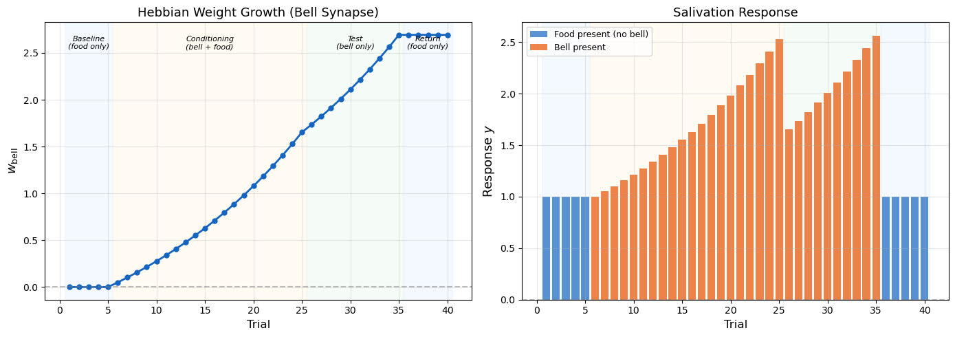
12.4b Hebbian Learning in Action: Classical Conditioning#

The Hebbian learning rule may seem abstract, so let us see it solve a real problem: classical conditioning — exactly the phenomenon Hebb set out to explain.

Pavlov’s Dog as a Neural Network#

In Pavlov’s famous experiment (1927), a dog learns to salivate at the sound of a bell after the bell is repeatedly paired with food. We can model this with a single neuron:

  food ──[w_food = 1.0 (innate)]──→ ╭──────╮
                                     │saliva│──→ y (response)
  bell ──[w_bell = 0.0 (learned)]──→ ╰──────╯

The food→saliva connection is innate (fixed weight \(w_{\text{food}} = 1\)).
The bell→saliva connection is initially zero (\(w_{\text{bell}} = 0\)).
Only the bell synapse learns via the Hebbian rule: \(\Delta w_{\text{bell}} = \eta \cdot \text{bell} \cdot y\).

Why It Works#

During conditioning, both bell and food are presented together:

\[y = w_{\text{food}} \cdot 1 + w_{\text{bell}} \cdot 1 = 1 + w_{\text{bell}} > 0\]

Since the bell is active (\(\text{bell} = 1\)) and the output is positive (\(y > 0\)), the Hebbian rule strengthens the bell synapse:

\[\Delta w_{\text{bell}} = \eta \cdot 1 \cdot y > 0\]

After enough pairings, \(w_{\text{bell}}\) grows large enough that the bell alone can drive the response — the network has learned to predict food from the bell.

Note

This is not merely an analogy. Hebb explicitly designed his rule to account for associative learning phenomena like classical conditioning. The simulation below shows the complete acquisition curve.

import numpy as np
import matplotlib.pyplot as plt

np.random.seed(42)

# ── Classical conditioning as Hebbian learning ──────────────────
# A single neuron learns to predict food from a bell signal.

eta = 0.05      # learning rate
n_trials = 40   # total trials

# Training protocol: (bell, food) per trial
# Phase 1: food only     (baseline — bell has no effect)
# Phase 2: bell + food   (conditioning — Hebbian pairing)
# Phase 3: bell only     (test — can the bell predict food?)
# Phase 4: food only     (the bell weight persists)
protocol = (
    [(0, 1)] * 5  +   # Phase 1: baseline (trials 1-5)
    [(1, 1)] * 20 +   # Phase 2: conditioning (trials 6-25)
    [(1, 0)] * 10 +   # Phase 3: test (trials 26-35)
    [(0, 1)] * 5       # Phase 4: return to food only (trials 36-40)
)

# Weights
w_food = 1.0    # innate (fixed) — hardwired response to food
w_bell = 0.0    # learned — initially no association

w_bell_history = [w_bell]
response_history = []

for bell, food in protocol:
    y = w_food * food + w_bell * bell   # neuron response
    response_history.append(y)
    w_bell += eta * bell * y            # Hebbian update (bell synapse only)
    w_bell_history.append(w_bell)

# ── Visualization ───────────────────────────────────────────────
fig, axes = plt.subplots(1, 2, figsize=(14, 5))

trials = np.arange(1, n_trials + 1)

# Phase background shading
phase_specs = [
    (1, 5,  '#E3F2FD', 'Baseline\n(food only)'),
    (6, 25, '#FFF3E0', 'Conditioning\n(bell + food)'),
    (26, 35,'#E8F5E9', 'Test\n(bell only)'),
    (36, 40,'#E3F2FD', 'Return\n(food only)'),
]

for ax in axes:
    for start, end, color, label in phase_specs:
        ax.axvspan(start - 0.5, end + 0.5, alpha=0.4, color=color)

# Panel 1: Learned weight w_bell
axes[0].plot(trials, w_bell_history[1:], 'o-', color='#1565C0',
             markersize=5, linewidth=2)
axes[0].set_xlabel('Trial', fontsize=12)
axes[0].set_ylabel(r'$w_{\mathrm{bell}}$', fontsize=13)
axes[0].set_title('Hebbian Weight Growth (Bell Synapse)', fontsize=13)
axes[0].axhline(y=0, color='gray', linestyle='--', alpha=0.5)
axes[0].grid(True, alpha=0.3)

# Phase labels
for start, end, _, label in phase_specs:
    axes[0].text((start + end) / 2, axes[0].get_ylim()[1] * 0.95,
                 label, ha='center', va='top', fontsize=8, style='italic')

# Panel 2: Neuron response
axes[1].bar(trials, response_history, color=[
    '#1565C0' if bell == 0 else '#E65100'
    for bell, food in protocol
], alpha=0.7, width=0.8)
axes[1].set_xlabel('Trial', fontsize=12)
axes[1].set_ylabel('Response $y$', fontsize=13)
axes[1].set_title('Salivation Response', fontsize=13)
axes[1].axhline(y=0, color='gray', linestyle='--', alpha=0.5)
axes[1].grid(True, alpha=0.3)

# Custom legend
from matplotlib.patches import Patch
axes[1].legend(handles=[
    Patch(facecolor='#1565C0', alpha=0.7, label='Food present (no bell)'),
    Patch(facecolor='#E65100', alpha=0.7, label='Bell present'),
], fontsize=9)

plt.tight_layout()
plt.show()

# Summary
print("Classical Conditioning via Hebbian Learning")
print("=" * 50)
print(f"  Baseline (bell only):     response = {w_bell_history[0]:.2f}  (no effect)")
print(f"  After conditioning:       w_bell   = {w_bell_history[25]:.2f}")
print(f"  Test (bell alone, trial 26): response = {response_history[25]:.2f}  (prediction!)")
print(f"  Final w_bell:             {w_bell_history[-1]:.2f}  (weight persists)")
print()
print("The network learned to PREDICT food from the bell signal.")
print("Note: w_bell keeps growing — this is the instability problem (§12.5)!")

../_images/b4992a83d7a4618301018629b337396fd9e75617e7fd72fb061e5cd334aaecf4.png

Classical Conditioning via Hebbian Learning
==================================================
  Baseline (bell only):     response = 0.00  (no effect)
  After conditioning:       w_bell   = 1.65
  Test (bell alone, trial 26): response = 1.65  (prediction!)
  Final w_bell:             2.69  (weight persists)

The network learned to PREDICT food from the bell signal.
Note: w_bell keeps growing — this is the instability problem (§12.5)!

What the Simulation Reveals#

The simulation demonstrates three fundamental properties of Hebbian learning:

Association through co-occurrence: The bell synapse strengthens because bell and response are repeatedly co-active during conditioning. This is Hebb’s rule at work.
Prediction without supervision: No teacher told the network that the bell predicts food. The association emerged purely from temporal co-occurrence — an unsupervised learning process.
The instability flaw: Notice that \(w_{\text{bell}}\) grows accelerating during conditioning — each trial makes the response larger, which makes the next update larger. During the test phase (bell only), the weight continues to grow even without food. This runaway growth is the instability problem we analyze next.

Warning

The simulation also reveals what Hebbian learning cannot do: there is no mechanism for extinction (unlearning). In real conditioning, presenting the bell without food eventually weakens the association. Pure Hebbian learning cannot weaken synapses — this requires extensions like LTD or the covariance rule (§12.6).

12.5 The Instability Problem#

Theorem (Weight Instability)

Under the basic Hebbian rule with stationary input statistics, the weight vector \(\mathbf{w}\) diverges to infinity: \(\|\mathbf{w}\| \to \infty\) as \(t \to \infty\).

Proof

Consider the continuous-time version of the Hebbian rule with a linear neuron:

\[\frac{d\mathbf{w}}{dt} = \eta \, y \, \mathbf{x} = \eta \, (\mathbf{w}^\top \mathbf{x}) \, \mathbf{x} = \eta \, \mathbf{x} \mathbf{x}^\top \mathbf{w}\]

Taking the expectation over the input distribution:

\[\frac{d\mathbf{w}}{dt} = \eta \, \mathbb{E}[\mathbf{x}\mathbf{x}^\top] \, \mathbf{w} = \eta \, \mathbf{C} \, \mathbf{w}\]

where \(\mathbf{C} = \mathbb{E}[\mathbf{x}\mathbf{x}^\top]\) is the input second-moment matrix; for centered data, this equals the covariance matrix.

Since \(\mathbf{C}\) is symmetric and positive semi-definite, it has an eigendecomposition:

\[\mathbf{C} = \sum_{i=1}^n \lambda_i \mathbf{e}_i \mathbf{e}_i^\top\]

where \(\lambda_1 \geq \lambda_2 \geq \cdots \geq \lambda_n \geq 0\) are the eigenvalues with corresponding orthonormal eigenvectors \(\mathbf{e}_1, \ldots, \mathbf{e}_n\).

Decomposing \(\mathbf{w}(t)\) in the eigenbasis:

\[\mathbf{w}(t) = \sum_{i=1}^n c_i(t) \, \mathbf{e}_i\]

Substituting into the differential equation:

\[\frac{dc_i}{dt} = \eta \lambda_i c_i\]

This has the solution:

\[c_i(t) = c_i(0) \, e^{\eta \lambda_i t}\]

Therefore:

\[\mathbf{w}(t) = \sum_{i=1}^n c_i(0) \, e^{\eta \lambda_i t} \, \mathbf{e}_i\]

For any eigenvalue \(\lambda_i > 0\) with nonzero initial component \(c_i(0) \neq 0\), the corresponding component grows exponentially. In particular:

\[\|\mathbf{w}(t)\| \geq |c_1(0)| \, e^{\eta \lambda_1 t} \to \infty \quad \text{as } t \to \infty\]

provided \(\lambda_1 > 0\) and \(c_1(0) \neq 0\). \(\blacksquare\)

Key insight: The weight vector grows fastest along the direction of the first eigenvector \(\mathbf{e}_1\) (the leading eigenvector of \(\mathbf{C}\); for centered data, the first principal component), but its norm diverges.

Danger

Pure Hebbian learning leads to unbounded weight growth! Without normalization, weights diverge to infinity. This is a fundamental flaw that took decades to resolve.

Show code cell source Hide code cell source

import numpy as np
import matplotlib.pyplot as plt

np.random.seed(42)

# Generate 2D correlated data
n_samples = 1000
# Correlation matrix with eigenvalues 2.0 and 0.5
angle = np.pi / 6  # 30 degrees
R = np.array([[np.cos(angle), -np.sin(angle)],
              [np.sin(angle),  np.cos(angle)]])
Lambda = np.diag([2.0, 0.5])
C = R @ Lambda @ R.T

# Generate data from this covariance
X = np.random.multivariate_normal([0, 0], C, n_samples)

# Basic Hebbian learning
eta = 0.001
w = np.array([0.5, 0.5])  # initial weights

# Track weight history
w_history = [w.copy()]
norm_history = [np.linalg.norm(w)]

n_epochs = 5
for epoch in range(n_epochs):
    for i in range(n_samples):
        x = X[i]
        y = w @ x          # linear output
        w = w + eta * y * x  # Hebbian update
        w_history.append(w.copy())
        norm_history.append(np.linalg.norm(w))

w_history = np.array(w_history)
norm_history = np.array(norm_history)

# Compute true principal component for reference
eigenvalues, eigenvectors = np.linalg.eigh(C)
pc1 = eigenvectors[:, -1]  # largest eigenvalue
print(f"True PC1 direction: {pc1}")
print(f"Final weight direction: {w / np.linalg.norm(w)}")
print(f"Final weight norm: {np.linalg.norm(w):.2f}")

# Plot
fig, axes = plt.subplots(1, 3, figsize=(16, 5))

# (1) Weight norm over time
axes[0].plot(norm_history)
axes[0].set_xlabel('Iteration')
axes[0].set_ylabel('||w||')
axes[0].set_title('Weight Norm (Exploding!)')
axes[0].set_yscale('log')
axes[0].grid(True, alpha=0.3)

# (2) Data with weight trajectory
axes[1].scatter(X[:, 0], X[:, 1], alpha=0.2, s=5, color='gray')
# Show weight direction at several time points
n_arrows = 10
indices = np.linspace(0, len(w_history)-1, n_arrows, dtype=int)
colors = plt.cm.viridis(np.linspace(0, 1, n_arrows))
for idx, color in zip(indices, colors):
    w_dir = w_history[idx] / np.linalg.norm(w_history[idx]) * 3
    axes[1].annotate('', xy=w_dir, xytext=[0, 0],
                     arrowprops=dict(arrowstyle='->', color=color, lw=2))
# Show true PC1
axes[1].annotate('', xy=pc1*3, xytext=[0, 0],
                 arrowprops=dict(arrowstyle='->', color='red', lw=2, linestyle='--'))
axes[1].set_xlabel('$x_1$')
axes[1].set_ylabel('$x_2$')
axes[1].set_title('Data and Weight Direction Over Time')
axes[1].set_aspect('equal')
axes[1].set_xlim(-5, 5)
axes[1].set_ylim(-5, 5)
axes[1].grid(True, alpha=0.3)
axes[1].legend(['PC1 (true)'], loc='upper left')

# (3) Angle to PC1 over time
angles = []
for w_t in w_history:
    cos_angle = np.abs(np.dot(w_t, pc1)) / (np.linalg.norm(w_t) * np.linalg.norm(pc1))
    cos_angle = np.clip(cos_angle, -1, 1)
    angles.append(np.degrees(np.arccos(cos_angle)))

axes[2].plot(angles)
axes[2].set_xlabel('Iteration')
axes[2].set_ylabel('Angle to PC1 (degrees)')
axes[2].set_title('Convergence of Direction to PC1')
axes[2].axhline(y=0, color='r', linestyle='--', alpha=0.5)
axes[2].grid(True, alpha=0.3)

plt.tight_layout()
plt.savefig('hebbian_instability.png', dpi=150, bbox_inches='tight')
plt.show()

print("\nKey observation: The weight DIRECTION converges to PC1,")
print("but the weight NORM diverges exponentially!")

True PC1 direction: [-0.8660254 -0.5      ]
Final weight direction: [0.87046814 0.49222476]
Final weight norm: 6905.93

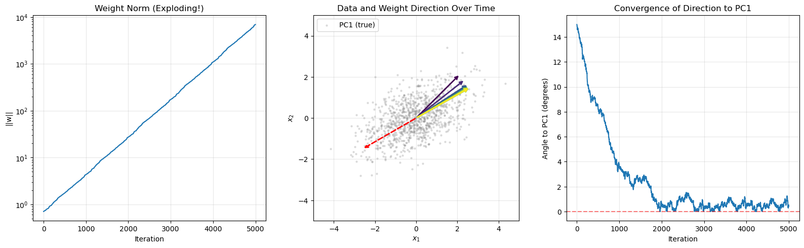
../_images/1413045bcb800742a5cc5f6deee3e98af0864fc32bf5e8822e88cfbde7be6049.png

Key observation: The weight DIRECTION converges to PC1,
but the weight NORM diverges exponentially!

Weight Growth Over Time: The Exponential Explosion#

The following visualization demonstrates the exponential weight growth under pure Hebbian learning for several different initial conditions and learning rates. The log-scale plot makes the exponential growth appear linear, confirming the theoretical prediction \(\|\mathbf{w}(t)\| \sim e^{\eta \lambda_1 t}\).

../_images/d543619af89628cf90aa54abc551fbe46f4b9d4636bee470cd313c3ae4ca34df.png

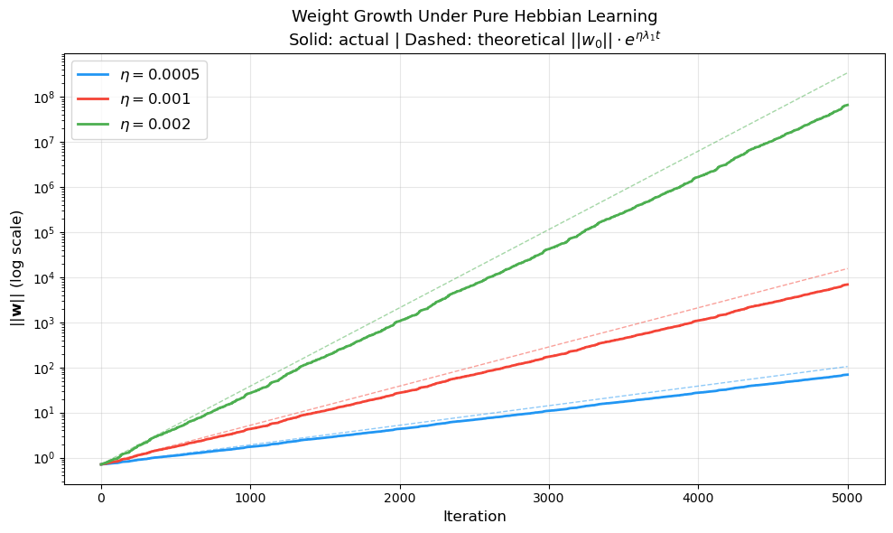
Largest eigenvalue lambda_1 = 2.000
Higher learning rates => faster exponential divergence.

12.6 The Covariance Rule#

One natural modification of the basic Hebbian rule is to use deviations from the means rather than raw activities:

\[\Delta w_{ij} = \eta (x_i - \bar{x}_i)(y_j - \bar{y}_j)\]

where \(\bar{x}_i = \mathbb{E}[x_i]\) and \(\bar{y}_j = \mathbb{E}[y_j]\) are the mean activities.

Properties#

Allows weakening: If \(x_i\) is above average but \(y_j\) is below average, the weight decreases. The basic Hebbian rule can only strengthen synapses (for positive activities).
Invariance to mean: The rule depends only on the covariance structure of the inputs and outputs, not their means.
Still unstable: The covariance rule inherits the instability problem of the basic Hebbian rule – weights still diverge.

The covariance rule is sometimes called the “centered Hebbian rule” and is closely related to PCA on centered data.

12.7 Biological Support for Hebbian Learning#

Long-Term Potentiation (LTP)#

The first direct evidence for Hebb’s postulate came 24 years after its publication.

Bliss & Lomo (1973) stimulated the perforant pathway in the hippocampus of anesthetized rabbits with high-frequency bursts (tetanic stimulation). They observed that synaptic transmission was enhanced for hours afterwards. This long-term potentiation (LTP) was the first experimental demonstration of a Hebbian synaptic modification.

The NMDA Receptor as a Coincidence Detector#

The molecular mechanism underlying LTP involves the NMDA receptor, which functions as an AND gate:

It requires glutamate binding (presynaptic activity).
It requires postsynaptic depolarization (to relieve the Mg\(^{2+}\) block).
Only when both conditions are met does Ca\(^{2+}\) flow in, triggering LTP.

This is precisely the coincidence detection Hebb described: the synapse strengthens only when the presynaptic neuron contributes to firing the postsynaptic neuron.

Long-Term Depression (LTD)#

Hebb’s original postulate only described strengthening. However, the brain also exhibits long-term depression (LTD) – weakening of synaptic connections. This occurs when:

Presynaptic activity occurs without sufficient postsynaptic response.
Low-frequency stimulation is applied.

LTD provides the weakening mechanism that the basic Hebbian rule lacks.

Spike-Timing-Dependent Plasticity (STDP)#

Note

Biological Evidence: STDP (Spike-Timing-Dependent Plasticity), discovered in the 1990s by Markram et al. (1997) and Bi & Poo (1998), confirms Hebb’s intuition with remarkable precision. STDP shows that the exact timing between pre- and postsynaptic spikes determines whether a synapse is strengthened or weakened – providing a temporally precise, causal version of Hebb’s “taking part in firing” condition.

A more refined view emerged with STDP, which depends on the precise timing between pre- and postsynaptic spikes:

\[\begin{split}\Delta w = \begin{cases} A_+ \exp\left(-\dfrac{\Delta t}{\tau_+}\right) & \text{if } \Delta t > 0 \text{ (pre before post: LTP)} \\ -A_- \exp\left(\dfrac{\Delta t}{\tau_-}\right) & \text{if } \Delta t < 0 \text{ (post before pre: LTD)} \end{cases}\end{split}\]

where \(\Delta t = t_{\text{post}} - t_{\text{pre}}\).

Typical values: \(\tau_+ \approx \tau_- \approx 20\) ms, \(A_+ \approx A_- \approx 0.01\).

../_images/e1832a089fe34e5c8d5cf6f47fb81ab986c1e809bc4eabc1645580f5712c2ef2.png

STDP Timing Window Curve#

The following visualization explores how the STDP curve changes with different parameter choices, showing the effect of varying the time constants \(\tau_+\), \(\tau_-\) and the amplitude ratio \(A_+/A_-\).

Show code cell source Hide code cell source

import numpy as np
import matplotlib.pyplot as plt

# STDP timing window curve: parameter exploration

dt = np.linspace(-100, 100, 2000)

fig, axes = plt.subplots(1, 3, figsize=(16, 5))

# Panel 1: Standard STDP window with biological parameters
params_list = [
    {'A_plus': 1.0, 'A_minus': 1.0, 'tau_plus': 20, 'tau_minus': 20, 'label': 'Symmetric ($A_+=A_-$)'},
    {'A_plus': 1.0, 'A_minus': 0.5, 'tau_plus': 20, 'tau_minus': 20, 'label': 'LTP-dominant ($A_+>A_-$)'},
    {'A_plus': 0.5, 'A_minus': 1.0, 'tau_plus': 20, 'tau_minus': 20, 'label': 'LTD-dominant ($A_+<A_-$)'},
]

for params in params_list:
    dw = np.where(dt > 0,
                  params['A_plus'] * np.exp(-dt / params['tau_plus']),
                  -params['A_minus'] * np.exp(dt / params['tau_minus']))
    dw[np.abs(dt) < 0.1] = 0
    axes[0].plot(dt, dw, linewidth=2, label=params['label'])

axes[0].axhline(y=0, color='gray', linewidth=0.5)
axes[0].axvline(x=0, color='gray', linewidth=0.5)
axes[0].set_xlabel(r'$\Delta t$ (ms)', fontsize=11)
axes[0].set_ylabel(r'$\Delta w$', fontsize=11)
axes[0].set_title('Effect of Amplitude Ratio', fontsize=12)
axes[0].legend(fontsize=9)
axes[0].grid(True, alpha=0.3)

# Panel 2: Effect of time constants
tau_values = [10, 20, 40]
colors = ['#E91E63', '#2196F3', '#4CAF50']
for tau, color in zip(tau_values, colors):
    dw = np.where(dt > 0,
                  1.0 * np.exp(-dt / tau),
                  -0.8 * np.exp(dt / tau))
    dw[np.abs(dt) < 0.1] = 0
    axes[1].plot(dt, dw, linewidth=2, color=color,
                label=f'$\\tau_\\pm = {tau}$ ms')

axes[1].axhline(y=0, color='gray', linewidth=0.5)
axes[1].axvline(x=0, color='gray', linewidth=0.5)
axes[1].set_xlabel(r'$\Delta t$ (ms)', fontsize=11)
axes[1].set_ylabel(r'$\Delta w$', fontsize=11)
axes[1].set_title('Effect of Time Constants', fontsize=12)
axes[1].legend(fontsize=10)
axes[1].grid(True, alpha=0.3)

# Panel 3: Net effect - integrate STDP over correlated pre/post spike trains
np.random.seed(42)
n_trials = 5000
correlation_values = np.linspace(-0.5, 1.0, 30)
net_dw = []

A_plus, A_minus = 1.0, 0.8
tau_plus, tau_minus = 20.0, 20.0

for corr in correlation_values:
    # Generate correlated spike time differences
    # Higher correlation -> more positive dt (pre before post)
    mean_dt = corr * 10  # mean time difference in ms
    dts = np.random.normal(mean_dt, 15, n_trials)
    
    dw_vals = np.where(dts > 0,
                       A_plus * np.exp(-dts / tau_plus),
                       -A_minus * np.exp(dts / tau_minus))
    net_dw.append(np.mean(dw_vals))

axes[2].plot(correlation_values, net_dw, 'k-', linewidth=2)
axes[2].fill_between(correlation_values, 0, net_dw,
                     where=[d > 0 for d in net_dw], alpha=0.3, color='green', label='Net LTP')
axes[2].fill_between(correlation_values, 0, net_dw,
                     where=[d <= 0 for d in net_dw], alpha=0.3, color='red', label='Net LTD')
axes[2].axhline(y=0, color='gray', linewidth=0.5)
axes[2].set_xlabel('Pre-Post Correlation', fontsize=11)
axes[2].set_ylabel(r'Net $\langle \Delta w \rangle$', fontsize=11)
axes[2].set_title('Net Weight Change vs Correlation', fontsize=12)
axes[2].legend(fontsize=10)
axes[2].grid(True, alpha=0.3)

plt.suptitle('STDP Timing Window: Parameter Exploration', fontsize=14, fontweight='bold', y=1.02)
plt.tight_layout()
plt.show()

print("Key insight: STDP is a temporally precise, causal version of Hebb's rule.")
print("Correlated firing (pre before post) leads to net potentiation.")

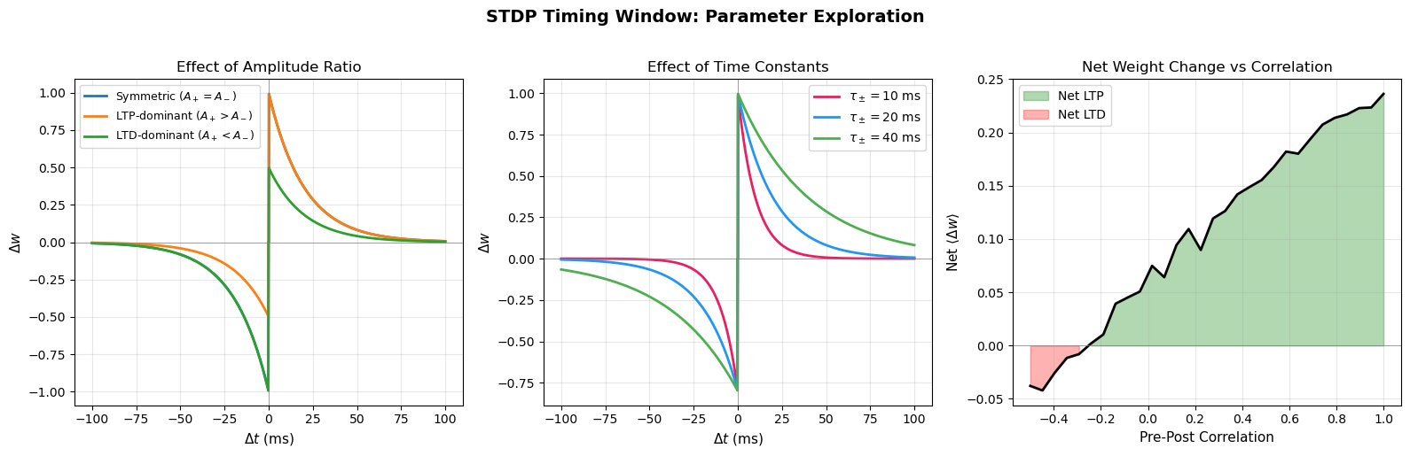
../_images/8df51cbd267d8542481ba82dde63cc5119364fd5102936055702706062fec317.png

Key insight: STDP is a temporally precise, causal version of Hebb's rule.
Correlated firing (pre before post) leads to net potentiation.

Hebbian Learning on Simple Patterns#

The following code demonstrates how the Hebbian weight matrix captures input correlations. We present several distinct patterns to a network of neurons and observe how the learned weight matrix reflects the correlation structure of the input data.

Show code cell source Hide code cell source

import numpy as np
import matplotlib.pyplot as plt

np.random.seed(42)

# Hebbian learning on simple patterns: weight matrix captures correlations

# Define 3 binary patterns (8-dimensional)
n_neurons = 8
patterns = np.array([
    [1, 1, 1, 1, 0, 0, 0, 0],   # Pattern A: first half active
    [0, 0, 0, 0, 1, 1, 1, 1],   # Pattern B: second half active
    [1, 0, 1, 0, 1, 0, 1, 0],   # Pattern C: alternating
], dtype=float)

# Convert to +1/-1 encoding for cleaner Hebbian learning
patterns_bipolar = 2 * patterns - 1

# Apply basic Hebbian learning: W = sum of outer products
W_hebb = np.zeros((n_neurons, n_neurons))
for p in patterns_bipolar:
    W_hebb += np.outer(p, p)

# Zero the diagonal (no self-connections)
np.fill_diagonal(W_hebb, 0)

# Also compute the true correlation matrix of the patterns
C_patterns = patterns_bipolar.T @ patterns_bipolar / len(patterns_bipolar)
np.fill_diagonal(C_patterns, 0)

# Online Hebbian learning with noisy presentations
eta = 0.01
W_online = np.zeros((n_neurons, n_neurons))
n_presentations = 3000

for _ in range(n_presentations):
    idx = np.random.randint(len(patterns_bipolar))
    x = patterns_bipolar[idx] + np.random.randn(n_neurons) * 0.1  # noisy
    # Hebbian: dW = eta * x * x^T
    W_online += eta * np.outer(x, x)

np.fill_diagonal(W_online, 0)

# Visualization
fig, axes = plt.subplots(1, 4, figsize=(18, 4))

# Panel 1: The patterns
im0 = axes[0].imshow(patterns_bipolar, cmap='RdBu_r', aspect='auto', vmin=-1.5, vmax=1.5)
axes[0].set_xlabel('Neuron index')
axes[0].set_ylabel('Pattern')
axes[0].set_yticks([0, 1, 2])
axes[0].set_yticklabels(['A', 'B', 'C'])
axes[0].set_title('Input Patterns', fontsize=12)
plt.colorbar(im0, ax=axes[0], shrink=0.8)

# Panel 2: Batch Hebbian weight matrix
im1 = axes[1].imshow(W_hebb, cmap='RdBu_r', aspect='equal')
axes[1].set_xlabel('Neuron j')
axes[1].set_ylabel('Neuron i')
axes[1].set_title('Batch Hebbian $W = \\sum \\mathbf{p}\\mathbf{p}^T$', fontsize=12)
plt.colorbar(im1, ax=axes[1], shrink=0.8)

# Panel 3: Online Hebbian weight matrix
im2 = axes[2].imshow(W_online, cmap='RdBu_r', aspect='equal')
axes[2].set_xlabel('Neuron j')
axes[2].set_ylabel('Neuron i')
axes[2].set_title('Online Hebbian (noisy)', fontsize=12)
plt.colorbar(im2, ax=axes[2], shrink=0.8)

# Panel 4: Pattern correlation matrix
im3 = axes[3].imshow(C_patterns, cmap='RdBu_r', aspect='equal')
axes[3].set_xlabel('Neuron j')
axes[3].set_ylabel('Neuron i')
axes[3].set_title('Pattern Correlation Matrix', fontsize=12)
plt.colorbar(im3, ax=axes[3], shrink=0.8)

plt.suptitle('Hebbian Learning Captures Correlation Structure',
             fontsize=14, fontweight='bold', y=1.02)
plt.tight_layout()
plt.show()

# Test pattern recall
print("Pattern recall test (using sign of W @ pattern):")
for i, (name, p) in enumerate(zip(['A', 'B', 'C'], patterns_bipolar)):
    recalled = np.sign(W_hebb @ p)
    match = np.all(recalled == p)
    print(f"  Pattern {name}: recalled correctly = {match}")

print("\nKey insight: The Hebbian weight matrix is proportional to the")
print("input correlation matrix. Neurons that co-activate in patterns")
print("develop strong positive connections (red), while anti-correlated")
print("neurons develop negative connections (blue).")

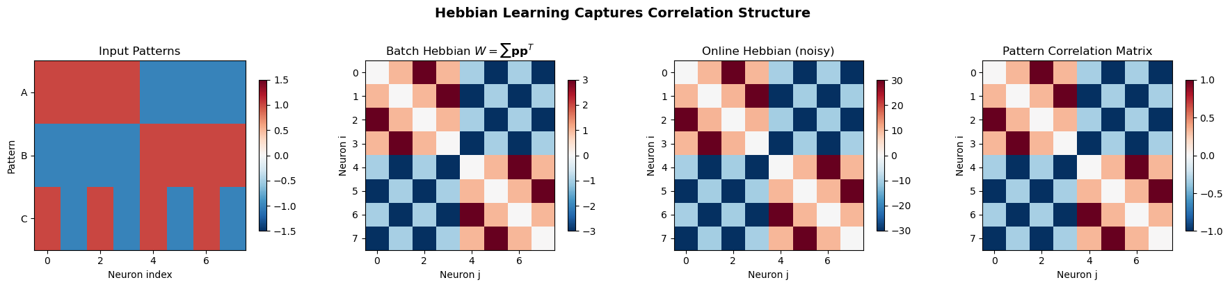
../_images/7c319a7baaf6abcad95befe259ef23fa1e25c15ff6ec18f21416048a8a6623db.png

Pattern recall test (using sign of W @ pattern):
  Pattern A: recalled correctly = True
  Pattern B: recalled correctly = True
  Pattern C: recalled correctly = True

Key insight: The Hebbian weight matrix is proportional to the
input correlation matrix. Neurons that co-activate in patterns
develop strong positive connections (red), while anti-correlated
neurons develop negative connections (blue).

12.8 Limitations of Hebbian Learning#

Despite its elegance and biological plausibility, Hebbian learning has significant limitations:

1. Unsupervised Only#

Hebbian learning is inherently unsupervised: it extracts statistical structure from inputs but cannot learn to map inputs to desired outputs. There is no mechanism for incorporating a target signal or error feedback.

2. No Credit Assignment#

In a multi-layer network, Hebbian learning provides no way to determine how hidden-layer weights should change to reduce output error. This is the credit assignment problem, which will be solved by backpropagation (Chapter 16).

3. Linear Projections Only#

With a linear neuron, Hebbian learning can only learn linear projections (principal components). It cannot learn nonlinear decision boundaries or nonlinear feature extraction.

4. Instability#

As proven in Section 12.5, basic Hebbian learning leads to unbounded weight growth. This requires modifications such as Oja’s rule (Chapter 13) or BCM theory (Chapter 14).

Summary#

Property	Hebbian Learning
Learning type	Unsupervised
Biological plausibility	High
Stability	Unstable (without modification)
What it learns	Principal components / correlations
Error signal needed	No
Can solve XOR	No
Credit assignment	No

Exercises#

Exercise 12.1. Implement the covariance rule \(\Delta w_{ij} = \eta(x_i - \bar{x}_i)(y_j - \bar{y}_j)\) using running estimates of the means. Compare its behavior with the basic Hebbian rule on data with nonzero mean.

Exercise 12.2. Prove that the weight direction under basic Hebbian learning converges to the leading eigenvector of \(\mathbf{C}\). That is, show \(\mathbf{w}(t)/\|\mathbf{w}(t)\| \to \pm \mathbf{e}_1\) as \(t \to \infty\), assuming \(|c_1(0)| > 0\) and \(\lambda_1 > \lambda_2\).

Exercise 12.3. Simulate STDP learning with Poisson spike trains. Generate pre- and postsynaptic spike trains at different rates and correlations. Compute the expected weight change and verify it matches the analytical prediction.

Exercise 12.4. What happens to Hebbian learning if the inputs are whitened (decorrelated with unit variance)? What does the correlation matrix \(\mathbf{C}\) become? What are the implications for the instability theorem?

Exercise 12.5. Implement Hebbian learning with a nonlinear activation function \(y = \tanh(\mathbf{w}^\top \mathbf{x})\). Does the saturation of tanh prevent unbounded weight growth? Run experiments to find out.

Chapter 12: Hebbian Learning Theory

Contents

Chapter 12: Hebbian Learning Theory#

12.1 Historical Context: Donald Hebb and the Birth of Synaptic Learning#

12.2 Hebb’s Postulate#

The Exact Statement#

The Popular Paraphrase#

Five Key Aspects of the Postulate#

12.3 Cell Assemblies and Phase Sequences#

12.4 The Basic Hebbian Learning Rule#

Mathematical Formulation#

Interpretation#

12.4b Hebbian Learning in Action: Classical Conditioning#

Pavlov’s Dog as a Neural Network#

Why It Works#

What the Simulation Reveals#

12.5 The Instability Problem#

Weight Growth Over Time: The Exponential Explosion#

12.6 The Covariance Rule#

Properties#

12.7 Biological Support for Hebbian Learning#

Long-Term Potentiation (LTP)#

The NMDA Receptor as a Coincidence Detector#

Long-Term Depression (LTD)#

Spike-Timing-Dependent Plasticity (STDP)#

STDP Timing Window Curve#

Hebbian Learning on Simple Patterns#

12.8 Limitations of Hebbian Learning#

1. Unsupervised Only#

2. No Credit Assignment#

3. Linear Projections Only#

4. Instability#

Summary#

Exercises#