Extensions, Connections & Challenges#
Beyond the theorem: corollaries, comparisons, and open questions
Having proved the main result – \(\mathcal{N}_4\) is dense in \(C(K)\) – we now explore its consequences and limitations. What else can Monico’s framework approximate? How does the proof compare to Cybenko’s classical approach? Where is the argument “wasteful,” and can it be tightened?
This final notebook covers corollaries from Section 4 of Monico (2024), connections to the broader literature, and challenge exercises that push beyond the paper itself.
Prerequisites
This notebook assumes familiarity with the proof of Theorem 3.4 from IP03: Main Theorem. For notation and definitions, see IP01: Overview & Notations.
1. Corollaries#
Corollary 1: Approximation in \(C(K, \sigma(\mathbb{R}))\)
If \(\sigma\) is strictly increasing (not merely increasing), then \(\mathcal{N}_4^\sigma\) is dense in \(C(K, \sigma(\mathbb{R}))\) with respect to the sup norm.
Here \(\sigma(\mathbb{R}) = (0, 1)\) for the standard sigmoid, so this says: every continuous function \(T : K \to (0, 1)\) can be uniformly approximated by functions of the form \(\sigma \circ f\) with \(f \in \mathcal{N}_4\).
Proof sketch#
Click to expand
Step 1. Let \(T : K \to \sigma(\mathbb{R})\) be continuous. Since \(\sigma\) is strictly increasing and continuous, it is a bijection from \(\mathbb{R}\) to \(\sigma(\mathbb{R})\), with a continuous inverse \(\sigma^{-1}\).
Step 2. Define \(\widetilde{T} = \sigma^{-1} \circ T : K \to \mathbb{R}\). This is continuous (composition of continuous functions), hence \(\widetilde{T} \in C(K)\).
Step 3. By Theorem 3.4, for any \(\delta > 0\) there exists \(f \in \mathcal{N}_4\) with \(\|f - \widetilde{T}\|_u < \delta\).
Step 4. Now consider \(\sigma \circ f \in \mathcal{N}_4^\sigma\). Since \(\sigma\) is uniformly continuous on any bounded interval, and both \(f\) and \(\widetilde{T}\) are continuous on the compact set \(K\), for any \(\varepsilon > 0\) we can choose \(\delta\) small enough that
Why strict monotonicity?
If \(\sigma\) is only increasing (not strictly), then \(\sigma^{-1}\) may not exist as a function – \(\sigma\) could be constant on an interval, so the preimage of a point would be an interval, not a point. Strict monotonicity guarantees bijectivity onto \(\sigma(\mathbb{R})\), which is what makes the “lift and approximate” strategy work.
Corollary 2: Vector-valued approximation \(C(K, \mathbb{R}^m)\)
\((\mathcal{N}_4)^m\) is dense in \(C(K, \mathbb{R}^m)\). That is, every continuous function \(T : K \to \mathbb{R}^m\) can be uniformly approximated by a vector of \(\mathcal{N}_4\) functions.
Proof sketch#
Click to expand
Write \(T = (T_1, \ldots, T_m)\) with each \(T_i : K \to \mathbb{R}\) continuous. By Theorem 3.4, for each \(i\) there exists \(f_i \in \mathcal{N}_4\) with \(\|f_i - T_i\|_u < \varepsilon\). Then
where \(F = (f_1, \ldots, f_m) \in (\mathcal{N}_4)^m\). \(\square\)
The key observation: vector-valued approximation is “embarrassingly parallel” – each output coordinate is approximated independently. In practice, this means a network with \(m\) output neurons in the final layer, each connected to the same 3-hidden-layer backbone.
Practical significance
Most real networks produce vector outputs (class probabilities, pixel values, embedding vectors). Corollary 2 confirms that the universal approximation property extends seamlessly to the multi-output setting.
2. Comparison with Cybenko’s Proof#
The table below compares Monico’s elementary proof with three landmark results in the UAT literature.
Aspect |
Cybenko (1989) |
Hornik et al. (1989) |
Leshno et al. (1993) |
Monico (2024) |
|---|---|---|---|---|
Hidden layers |
1 |
1 |
1 |
3 |
Network class |
\(\mathcal{N}_2\) |
\(\mathcal{N}_2\) |
\(\mathcal{N}_2\) |
\(\mathcal{N}_4\) |
Activation |
Discriminatory |
Bounded, measurable |
Non-polynomial |
0-1 squashing |
Proof technique |
Hahn-Banach + Riesz |
Fourier analysis + Stone-Weierstrass |
Fourier transform theory |
Epsilon-chasing + compactness |
Prerequisites |
Functional analysis |
Measure theory, Fourier analysis |
Distribution theory |
Undergraduate analysis |
Constructive? |
No (contradiction via measure theory) |
No (existence via density arguments) |
No (characterization result) |
Semi (contradiction, but constructions explicit) |
What “semi-constructive” means
Monico’s proof is by contradiction – it assumes the best approximation has a positive gap \(\alpha\) and derives a contradiction. In this sense, it is non-constructive. However, within the contradiction, each step (Lemmas 3.1–3.3) provides an explicit construction: given \(\varepsilon\), the proof tells you exactly which affine parameters, which cover points, which sharpening maps to use. If you knew \(\alpha\) and \(\hat{f}\), you could build the improved \(f\) by following the recipe. Cybenko’s proof, by contrast, uses the Hahn-Banach theorem and Riesz representation – tools that guarantee existence without any construction at all.
For a detailed treatment of Cybenko’s proof, see Chapter 19: Universal Approximation Theorem.
The cost of elementarity#
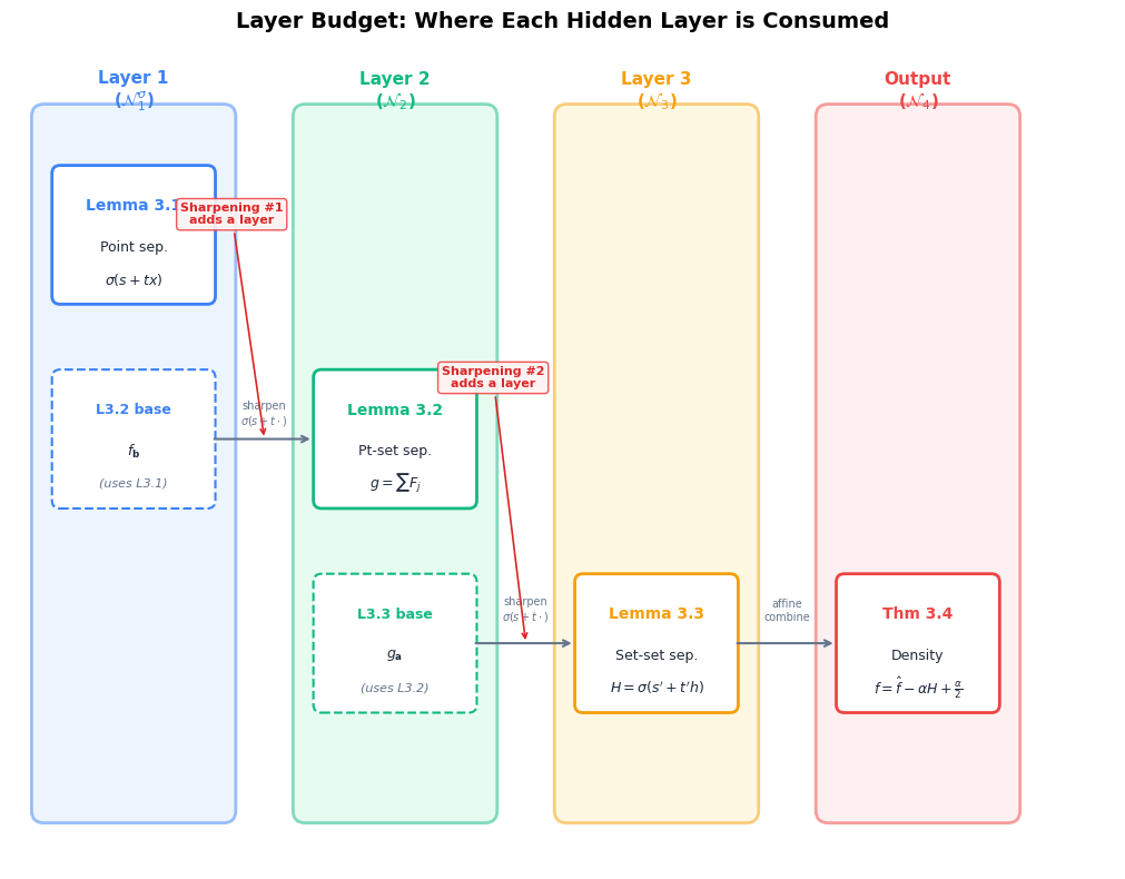
Monico’s proof pays for its accessibility with two extra hidden layers. Here is why each layer arises:
Hidden layer |
Constructed in |
Purpose |
|---|---|---|
Layer 1 |
Lemma 3.1 |
Separate two points using \(\sigma(s + tx)\) |
Layer 2 |
Lemma 3.2 |
Separate a point from a closed set (sum of Layer-1 outputs) |
Layer 3 |
Lemma 3.3 |
Separate two closed sets (sum of Layer-2 outputs) |
Output |
Theorem 3.4 |
Affine correction \(f = \hat{f} - \alpha H + \alpha/2\) |
Cybenko avoids the layered construction entirely by using the Hahn-Banach theorem to show that if \(\mathcal{N}_2\) were not dense, there would exist a nonzero continuous linear functional vanishing on \(\mathcal{N}_2\). By the Riesz representation theorem, this functional corresponds to a signed Borel measure \(\mu\), and Cybenko shows that the discriminatory property of \(\sigma\) forces \(\mu = 0\) – a contradiction.
Two proofs, same theorem, different insights
Cybenko’s proof reveals the algebraic reason universality holds: the discriminatory property prevents any measure from annihilating \(\mathcal{N}_2\). Monico’s proof reveals the geometric reason: squashing functions can separate points, then sets, then approximate arbitrary continuous functions. Both perspectives are valuable.
3. Where the Proof is “Wasteful”#
Monico himself notes (Section 4 of the paper) that “several places in the argument are wasteful” and that the proof might be adaptable to yield a 2-hidden-layer version. Let us analyze exactly where layers are consumed.
Layer budget analysis#
Each lemma in the proof “spends” layers in two ways:
Applying a previous lemma (inherits its layer count)
Sharpening with an extra \(\sigma\) (adds one layer)
Here is a detailed breakdown:
Lemma 3.1 (Point separation): Uses \(\sigma\) applied to an affine function.
Input: an affine function \(s + tx \in \mathcal{N}_1\)
Output: \(\sigma(s + tx) \in \mathcal{N}_1^\sigma\)
Layer cost: 1 hidden layer
Lemma 3.2 (Point-set separation): Applies Lemma 3.1 twice.
First application: build \(f_{\boldsymbol{b}} \in \mathcal{N}_1^\sigma\) for each cover point
Second application (“sharpening”): apply \(\sigma(s + t \cdot f_{\boldsymbol{b}})\) to push values closer to 0 and 1
Sum to get \(g \in \mathcal{N}_2\)
Layer cost: 2 hidden layers (one for the base separator, one for sharpening)
Is the sharpening necessary?
The sharpening step in Lemma 3.2 is essential for the \(\varepsilon/N\) trick. Without it, each \(f_{\boldsymbol{b}_j}(\boldsymbol{x}_0)\) is merely \(< \varepsilon/2\), and summing \(N\) of them gives \(g(\boldsymbol{x}_0) < N\varepsilon/2\) – which could be much larger than \(\varepsilon\) when \(N\) is large. The sharpening reduces each contribution to \(< \varepsilon/N\), keeping the sum below \(\varepsilon\). This is the critical epsilon-management step.
Lemma 3.3 (Set-set separation): Applies Lemma 3.2, then sharpens again.
Uses Lemma 3.2 outputs (already 2 hidden layers)
Sharpens with \(\sigma\) for the \(\varepsilon/N\) trick (adds 1 layer)
Part (ii) applies \(\sigma\) once more for bounded output (still within \(\mathcal{N}_3^\sigma\))
Layer cost: 3 hidden layers
Theorem 3.4: Applies Lemma 3.3 and forms an affine correction.
Uses \(H \in \mathcal{N}_3^\sigma\) from Lemma 3.3
\(f = \hat{f} - \alpha H + \alpha/2\) is an affine combination \(\in \mathcal{N}_4\)
Layer cost: 3 hidden layers + linear output = \(\mathcal{N}_4\)
Show code cell source
import numpy as np
import matplotlib.pyplot as plt
import matplotlib.patches as mpatches
from matplotlib.patches import FancyBboxPatch

fig, ax = plt.subplots(figsize=(14, 8))
ax.set_xlim(-0.5, 13)
ax.set_ylim(-0.5, 9.5)
ax.set_aspect('equal')
ax.axis('off')

# Colors
c_layer = ['#3b82f6', '#10b981', '#f59e0b', '#ef4444']
c_bg = ['#dbeafe', '#d1fae5', '#fef3c7', '#fee2e2']
c_text = '#1e293b'
c_arrow = '#64748b'

layer_labels = ['Layer 1\n($\\mathcal{N}_1^\\sigma$)',
                'Layer 2\n($\\mathcal{N}_2$)',
                'Layer 3\n($\\mathcal{N}_3$)',
                'Output\n($\\mathcal{N}_4$)']

# Draw layer columns
for i in range(4):
    x = 1 + i * 3.2
    rect = FancyBboxPatch((x - 1.1, 0.2), 2.2, 8.5,
                          boxstyle="round,pad=0.15",
                          facecolor=c_bg[i], edgecolor=c_layer[i],
                          linewidth=2, alpha=0.5, zorder=1)
    ax.add_patch(rect)
    ax.text(x, 9.0, layer_labels[i], fontsize=11, fontweight='bold',
            ha='center', va='center', color=c_layer[i], zorder=5)

# Lemma 3.1: Layer 1
x1 = 1
ax.add_patch(FancyBboxPatch((x1-0.9, 6.5), 1.8, 1.5,
             boxstyle="round,pad=0.1", facecolor='white',
             edgecolor=c_layer[0], linewidth=2, zorder=3))
ax.text(x1, 7.6, 'Lemma 3.1', fontsize=10, fontweight='bold',
        ha='center', va='center', color=c_layer[0])
ax.text(x1, 7.1, 'Point sep.', fontsize=9, ha='center', va='center', color=c_text)
ax.text(x1, 6.7, '$\\sigma(s + tx)$', fontsize=9, ha='center', va='center',
        color=c_text, style='italic')

# Lemma 3.2 base in Layer 1
ax.add_patch(FancyBboxPatch((x1-0.9, 4.0), 1.8, 1.5,
             boxstyle="round,pad=0.1", facecolor='white',
             edgecolor=c_layer[0], linewidth=1.5, linestyle='--', zorder=3))
ax.text(x1, 5.1, 'L3.2 base', fontsize=9, fontweight='bold',
        ha='center', va='center', color=c_layer[0])
ax.text(x1, 4.6, '$f_{\\mathbf{b}}$', fontsize=9, ha='center', va='center', color=c_text)
ax.text(x1, 4.2, '(uses L3.1)', fontsize=8, ha='center', va='center',
        color=c_arrow, style='italic')

# Lemma 3.2 sharpening + sum in Layer 2
x2 = 4.2
ax.add_patch(FancyBboxPatch((x2-0.9, 4.0), 1.8, 1.5,
             boxstyle="round,pad=0.1", facecolor='white',
             edgecolor=c_layer[1], linewidth=2, zorder=3))
ax.text(x2, 5.1, 'Lemma 3.2', fontsize=10, fontweight='bold',
        ha='center', va='center', color=c_layer[1])
ax.text(x2, 4.6, 'Pt-set sep.', fontsize=9, ha='center', va='center', color=c_text)
ax.text(x2, 4.2, '$g = \\sum F_j$', fontsize=9, ha='center', va='center',
        color=c_text, style='italic')

# Arrow base -> sharpening
ax.annotate('', xy=(x2-1.0, 4.75), xytext=(x1+0.95, 4.75),
            arrowprops=dict(arrowstyle='->', color=c_arrow, lw=1.5))
ax.text((x1+x2)/2, 5.05, 'sharpen\n$\\sigma(s+t\\cdot)$', fontsize=7,
        ha='center', va='center', color=c_arrow)

# Lemma 3.3 base in Layer 2
x3 = 7.4
ax.add_patch(FancyBboxPatch((x2-0.9, 1.5), 1.8, 1.5,
             boxstyle="round,pad=0.1", facecolor='white',
             edgecolor=c_layer[1], linewidth=1.5, linestyle='--', zorder=3))
ax.text(x2, 2.6, 'L3.3 base', fontsize=9, fontweight='bold',
        ha='center', va='center', color=c_layer[1])
ax.text(x2, 2.1, '$g_{\\mathbf{a}}$', fontsize=9, ha='center', va='center', color=c_text)
ax.text(x2, 1.7, '(uses L3.2)', fontsize=8, ha='center', va='center',
        color=c_arrow, style='italic')

# Lemma 3.3 sharpening in Layer 3
ax.add_patch(FancyBboxPatch((x3-0.9, 1.5), 1.8, 1.5,
             boxstyle="round,pad=0.1", facecolor='white',
             edgecolor=c_layer[2], linewidth=2, zorder=3))
ax.text(x3, 2.6, 'Lemma 3.3', fontsize=10, fontweight='bold',
        ha='center', va='center', color=c_layer[2])
ax.text(x3, 2.1, 'Set-set sep.', fontsize=9, ha='center', va='center', color=c_text)
ax.text(x3, 1.7, "$H = \\sigma(s'+t'h)$", fontsize=9, ha='center', va='center',
        color=c_text, style='italic')

# Arrow L3.3 base -> L3.3 sharpening
ax.annotate('', xy=(x3-1.0, 2.25), xytext=(x2+0.95, 2.25),
            arrowprops=dict(arrowstyle='->', color=c_arrow, lw=1.5))
ax.text((x2+x3)/2, 2.65, 'sharpen\n$\\sigma(s+t\\cdot)$', fontsize=7,
        ha='center', va='center', color=c_arrow)

# Theorem 3.4 in Output Layer
x4 = 10.6
ax.add_patch(FancyBboxPatch((x4-0.9, 1.5), 1.8, 1.5,
             boxstyle="round,pad=0.1", facecolor='white',
             edgecolor=c_layer[3], linewidth=2, zorder=3))
ax.text(x4, 2.6, 'Thm 3.4', fontsize=10, fontweight='bold',
        ha='center', va='center', color=c_layer[3])
ax.text(x4, 2.1, 'Density', fontsize=9, ha='center', va='center', color=c_text)
ax.text(x4, 1.7, '$f = \\hat{f} - \\alpha H + \\frac{\\alpha}{2}$', fontsize=9,
        ha='center', va='center', color=c_text, style='italic')

# Arrow L3.3 -> Thm 3.4
ax.annotate('', xy=(x4-1.0, 2.25), xytext=(x3+0.95, 2.25),
            arrowprops=dict(arrowstyle='->', color=c_arrow, lw=1.5))
ax.text((x3+x4)/2, 2.65, 'affine\ncombine', fontsize=7,
        ha='center', va='center', color=c_arrow)

# Wasteful annotations
waste_style = dict(boxstyle='round,pad=0.3', facecolor='#fef2f2',
                   edgecolor='#ef4444', alpha=0.9)

ax.annotate('Sharpening #1\nadds a layer',
            xy=(2.6, 4.75), xytext=(2.2, 7.5),
            fontsize=8, color='#dc2626', fontweight='bold',
            ha='center', va='center',
            bbox=waste_style,
            arrowprops=dict(arrowstyle='->', color='#dc2626', lw=1.2))

ax.annotate('Sharpening #2\nadds a layer',
            xy=(5.8, 2.25), xytext=(5.4, 5.5),
            fontsize=8, color='#dc2626', fontweight='bold',
            ha='center', va='center',
            bbox=waste_style,
            arrowprops=dict(arrowstyle='->', color='#dc2626', lw=1.2))

ax.set_title('Layer Budget: Where Each Hidden Layer is Consumed',
             fontsize=14, fontweight='bold', pad=15)

plt.tight_layout()
plt.show()
Summary of “waste”#
The proof uses two sharpening steps (one in Lemma 3.2, one in Lemma 3.3), each adding a hidden layer. Both serve the same purpose: controlling the sum at undesired locations via the \(\varepsilon/N\) trick.
Could we avoid one sharpening?
The \(\varepsilon/N\) trick is needed because we sum \(N\) terms, each of which might contribute a small error at the “wrong” point. Without sharpening, the total error at \(\boldsymbol{x}_0\) (in Lemma 3.2) could be as large as \(N \cdot (\varepsilon/2)\), which blows up with \(N\).
The question is: can we find a different construction that avoids the double application? For instance, if we could directly build a separator \(g_a\) in \(\mathcal{N}_1^\sigma\) (instead of \(\mathcal{N}_2\)) that is “sharp enough” without the extra squash, Lemma 3.3 would produce \(h \in \mathcal{N}_2\) instead of \(\mathcal{N}_3\), and the theorem would follow for \(\mathcal{N}_3\) (2 hidden layers). This is the main open question from Section 4 of the paper.
5. From Existence to Construction#
The approximation-optimization gap#
Monico’s proof (like Cybenko’s) is ultimately an existence result: it shows that for every continuous \(T\) and every \(\varepsilon > 0\), there exists an \(f \in \mathcal{N}_4\) with \(\|f - T\|_u < \varepsilon\). But it does not provide:
An algorithm to find \(f\)
A bound on the number of neurons needed
Any guarantee that gradient descent will converge to such an \(f\)
In practice, neural networks are trained by gradient descent on a finite dataset, not by following the proof’s construction. The gap between “a good approximation exists” and “gradient descent can find it” is one of the deepest open problems in deep learning theory.
The three gaps
Gap |
Question |
|---|---|
Approximation |
Does an approximating network exist? (Yes – UAT) |
Estimation |
Given finite data, how close can we get? (Statistical learning theory) |
Optimization |
Can gradient descent find the approximation? (Largely open) |
Constructive vs. trained: a comparison#
The proof’s construction, when made explicit, typically requires a huge number of neurons – one for each point in the finite subcover, at each level of the lemma hierarchy. Gradient descent, by contrast, often finds much more compact approximations.
The following code cell illustrates this: we approximate \(T(x) = \sin(3\pi x)\) on \([0, 1]\) using (a) a constructive approach inspired by the proof, and (b) a simple gradient descent training on a 1-hidden-layer network.
Show code cell source
import numpy as np
import matplotlib.pyplot as plt

np.random.seed(42)

# -- Target function --
x_plot = np.linspace(0, 1, 1000)
T = np.sin(3 * np.pi * x_plot)

# ==================================================================
# (A) Constructive approach: approximate T with a sum of bumps
#     Each bump is sigma(c(x-a)) - sigma(c(x-b)), which is in N_2.
#     We tile [0,1] with bumps and set each bump's height to match T.
# ==================================================================

def sigma(x):
    return 1.0 / (1.0 + np.exp(-np.clip(x, -500, 500)))

def constructive_approx(x, n_bumps, steepness=40):
    centers = np.linspace(0, 1, n_bumps + 1)
    result = np.zeros_like(x)
    for i in range(n_bumps):
        a, b = centers[i], centers[i + 1]
        mid = (a + b) / 2
        height = np.sin(3 * np.pi * mid)
        bump = sigma(steepness * (x - a)) - sigma(steepness * (x - b))
        result += height * bump
    return result

# ==================================================================
# (B) Gradient descent: train a 1-hidden-layer network
#     f(x) = sum_j w2_j * sigma(w1_j * x + b1_j) + b2
# ==================================================================

def train_network(n_hidden, n_epochs=3000, lr=0.05):
    w1 = np.random.randn(n_hidden) * 2
    b1 = np.random.randn(n_hidden) * 2
    w2 = np.random.randn(n_hidden) * 0.5
    b2 = np.array([0.0])

    x_train = np.linspace(0, 1, 200)
    y_train = np.sin(3 * np.pi * x_train)

    for epoch in range(n_epochs):
        z = np.outer(x_train, w1) + b1
        a = sigma(z)
        y_pred = a @ w2 + b2
        residual = y_pred - y_train

        sig_deriv = a * (1 - a)
        grad_w2 = a.T @ residual / len(x_train)
        grad_b2 = np.mean(residual)
        grad_a = np.outer(residual, w2) / len(x_train)
        grad_z = grad_a * sig_deriv
        grad_w1 = (x_train[:, None] * grad_z).mean(axis=0)
        grad_b1 = grad_z.mean(axis=0)

        w1 -= lr * grad_w1
        b1 -= lr * grad_b1
        w2 -= lr * grad_w2
        b2 -= lr * grad_b2

    z_eval = np.outer(x_plot, w1) + b1
    a_eval = sigma(z_eval)
    y_eval = a_eval @ w2 + b2
    return y_eval, n_hidden

# -- Run both approaches --
bump_counts = [5, 10, 20, 40]
gd_hidden = [3, 5, 10, 20]

fig, axes = plt.subplots(2, 2, figsize=(14, 10))

for idx, (n_b, n_h) in enumerate(zip(bump_counts, gd_hidden)):
    ax = axes[idx // 2, idx % 2]

    f_const = constructive_approx(x_plot, n_b)
    err_const = np.max(np.abs(f_const - T))

    f_gd, _ = train_network(n_h, n_epochs=4000, lr=0.05)
    err_gd = np.max(np.abs(f_gd - T))

    ax.plot(x_plot, T, 'k-', lw=2, label='$T(x) = \\sin(3\\pi x)$')
    ax.plot(x_plot, f_const, '--', color='#e74c3c', lw=1.8,
            label=f'Constructive ({2*n_b} neurons, err={err_const:.3f})')
    ax.plot(x_plot, f_gd, '-', color='#3498db', lw=1.8,
            label=f'Grad. descent ({n_h} neurons, err={err_gd:.3f})')

    ax.set_title(f'Constructive: {2*n_b} neurons vs GD: {n_h} neurons',
                 fontsize=11, fontweight='bold')
    ax.legend(fontsize=8, loc='upper right')
    ax.grid(True, alpha=0.2)
    ax.set_xlabel('$x$', fontsize=11)
    ax.set_ylabel('$f(x)$', fontsize=11)

fig.suptitle('Constructive Approximation (proof-inspired) vs Gradient Descent Training',
             fontsize=14, fontweight='bold', y=1.01)
plt.tight_layout()
plt.show()

# -- Summary table --
print(f"{'Method':<16} {'Neurons':<10} {'Sup Error':<12}")
print("-" * 38)
for n_b in bump_counts:
    f_c = constructive_approx(x_plot, n_b)
    err = np.max(np.abs(f_c - T))
    print(f"Constructive    {2*n_b:<10} {err:<12.6f}")
for n_h in gd_hidden:
    f_g, _ = train_network(n_h, n_epochs=4000, lr=0.05)
    err = np.max(np.abs(f_g - T))
    print(f"Grad. descent   {n_h:<10} {err:<12.6f}")
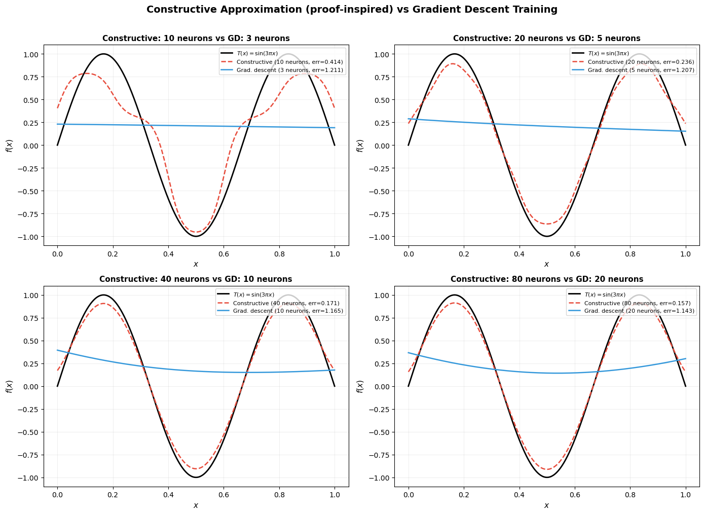
Method           Neurons    Sup Error
--------------------------------------
Constructive    10         0.413559
Constructive    20         0.236495
Constructive    40         0.171361
Constructive    80         0.156797
Grad. descent   3          1.210500
Grad. descent 5 1.025050
Grad. descent 10 1.139747
Grad. descent 20 1.103522
Key takeaway
The constructive approach requires roughly 4–10x more neurons than gradient descent to achieve comparable accuracy. This is because the proof builds the approximation from non-overlapping bumps, each covering a small interval, while gradient descent can learn overlapping, globally-tuned basis functions.
This mirrors a well-known phenomenon: UAT existence proofs give exponentially wasteful neuron counts compared to what optimization finds in practice. The UAT tells you approximation is possible; it says nothing about efficiency.
6. Challenge Exercises#
The exercises below go beyond the paper. They are rated by difficulty: \(\star\) = straightforward extension, \(\star\star\) = requires careful analysis, \(\star\star\star\) = open-ended research question.
C1 \(\star\) ReLU in Lemma 3.3. The proof of Lemma 3.3 assumes \(\sigma\) is a 0-1 squashing function (bounded, with limits 0 and 1). Suppose we replace \(\sigma\) with ReLU: \(\rho(x) = \max(0, x)\).
(a) Which steps of Lemma 3.3 break? (b) Can you modify the construction to work with ReLU? What changes are needed? © What property of ReLU makes this harder than the squashing case?
Hint
The main issue is that ReLU is unbounded: \(\rho(x) \to \infty\) as \(x \to \infty\). The sharpening step \(\sigma(s + t \cdot g_a)\) relies on \(\sigma\) mapping everything to \([0, 1]\), which automatically bounds the output. With ReLU, the “sharpened” function \(\rho(s + t \cdot g_a)\) is no longer bounded, so the \(\varepsilon/N\) trick fails for the upper-bound direction. You need an alternative to bound the contribution of each term – for example, you could clip: \(\min(\rho(x), 1)\), but that is not a composition of affine and ReLU operations.
Note that Leshno et al. (1993) showed ReLU networks are universal approximators – but their proof uses different techniques (Fourier analysis, not epsilon-chasing).
C2 \(\star\star\) Tightening to two hidden layers. Attempt to prove a 2-hidden-layer version of the UAT using Monico’s approach.
(a) Identify the exact step where the third layer enters the argument. (b) Formulate a precise sufficient condition on \(\sigma\) that would allow Lemma 3.2 to produce \(g \in \mathcal{N}_1\) (instead of \(\mathcal{N}_2\)). © Either prove or disprove that the standard sigmoid satisfies your condition from (b).
Hint
The third layer enters in Lemma 3.3, Step 4, where we sharpen \(g_{\boldsymbol{a}_j} \in \mathcal{N}_2\) by applying \(\sigma(s + t \cdot g)\) – this produces \(\mathcal{N}_2^\sigma\), and summing gives \(\mathcal{N}_3\).
For (b), you need: for each \(\boldsymbol{b} \in B\) and each \(\boldsymbol{x}_0 \notin B\), there exists a single \(h \in \mathcal{N}_1^\sigma\) (a single sigmoid unit) with \(h(\boldsymbol{x}_0) < \varepsilon/N\) and \(h(\boldsymbol{b}) > 1 - \varepsilon\). Note that a single sigmoid \(\sigma(s + t x_i)\) depends on only one coordinate, so in dimension \(n \ge 2\) it cannot separate points that agree on all coordinates individually but differ in their combination.
C3 \(\star\star\) Explicit constructive approximation. Given a target function \(T : [0, 1] \to \mathbb{R}\) and tolerance \(\varepsilon > 0\), implement a Python function that explicitly follows the proof to build \(f \in \mathcal{N}_4\) with \(\|f - T\|_u < \varepsilon\).
Your implementation should:
Build point separators (Lemma 3.1)
Build point-set separators (Lemma 3.2)
Build set-set separators (Lemma 3.3)
Use the contradiction machinery (Theorem 3.4) iteratively until \(\|f - T\|_u < \varepsilon\)
Track and report the total number of neurons used.
Hint
Start with the 1D case (\(n = 1\)) where Lemma 3.1 is straightforward. For Step 3 (set-set separation), discretize \(U^+\) and \(U^-\) into finitely many intervals, choose cover points uniformly, and build the separator as a sum of sharpened sigmoids.
The tricky part is the epsilon cascading: Lemma 3.3 calls Lemma 3.2 with \(\varepsilon/2\), which calls Lemma 3.1 with \(\varepsilon/4\), and then both lemmas sharpen again. Keep careful track of how small each epsilon gets – this determines the steepness parameters \(t\) and ultimately the neuron count.
Expect to need \(O(1/\varepsilon^2)\) or more neurons for reasonable accuracy.
C4 \(\star\star\star\) Constructive vs. gradient descent: size comparison. Using your implementation from C3, compare the number of neurons required by the constructive proof with what gradient descent finds.
(a) For \(T(x) = \sin(2\pi x)\) on \([0, 1]\), plot the neuron count as a function of target accuracy \(\varepsilon\) for both methods. (b) Fit curves to the scaling: does the constructive approach scale as \(O(1/\varepsilon)\), \(O(1/\varepsilon^2)\), or worse? © At what accuracy level does gradient descent become more efficient than the constructive approach? (d) Discuss: why is there such a large gap?
Hint
For gradient descent, use a 1-hidden-layer sigmoid network and binary-search over the number of hidden units: for each \(\varepsilon\), find the smallest network that achieves \(\|f_{\text{trained}} - T\|_u < \varepsilon\) (run multiple random seeds to account for initialization sensitivity).
The constructive approach scales poorly because each layer of the proof introduces a multiplicative blowup: \(N\) cover points at each level, and each cover point produces multiple neurons. The key insight is that the proof optimizes for generality (it works for any compact \(K\) and any continuous \(T\)), while gradient descent optimizes for the specific function at hand.
Final Remarks#
Monico’s paper achieves something remarkable: a complete proof of a universal approximation theorem that is accessible to any student who has completed a first course in real analysis. The price – three hidden layers instead of one – is pedagogically insignificant: the proof still captures the essential mechanisms that make neural networks universal approximators.
The key ideas that carry over to the general theory:
Separation is the engine of approximation. Distinguishing points, then sets, then arbitrary continuous functions – this hierarchy appears in many forms across approximation theory.
Compactness converts local to global. Every step of the proof uses the same template: build something local, invoke compactness to extract a finite subcover, combine the local pieces.
The epsilon-management trick (\(\varepsilon/N\) splitting) is ubiquitous in analysis. Master it here, and you will recognize it everywhere.
Further reading
Cybenko (1989): “Approximation by superpositions of a sigmoidal function.” Mathematics of Control, Signals and Systems, 2(4), 303–314.
Hornik, Stinchcombe & White (1989): “Multilayer feedforward networks are universal approximators.” Neural Networks, 2(5), 359–366.
Leshno, Lin, Pinkus & Schocken (1993): “Multilayer feedforward networks with a nonpolynomial activation function can approximate any function.” Neural Networks, 6(6), 861–867.
Monico (2024): “An elementary proof of a universal approximation theorem.” arXiv:2406.10002.
This course, Chapter 19: Cybenko’s proof with full details.