Chapter 13: Oja’s Rule and Principal Component Analysis#
In Chapter 12, we saw that the basic Hebbian rule causes the weight vector to align with the leading eigenvector of the input second-moment matrix (for centered data, the first principal component), but its norm diverges to infinity. In this chapter, we study Oja’s rule (1982), an elegant modification that solves the instability problem while preserving the desirable convergence to the principal component direction.
13.1 Oja’s Rule#
Definition (Oja’s Rule, 1982)
Oja’s rule modifies the basic Hebbian rule by adding a weight decay term proportional to the square of the output:
where \(y = \mathbf{w}^\top \mathbf{x}\) is the linear output and \(\eta > 0\) is the learning rate.
Component-wise:
The first term \(y\mathbf{x}\) is the standard Hebbian term. The second term \(-y^2 \mathbf{w}\) is a weight decay that prevents the norm from growing without bound.
Tip
The key insight – the \(-y^2 w\) term provides automatic weight normalization, preventing the instability of pure Hebbian learning. When \(\|\mathbf{w}\|\) grows too large, the output \(y\) becomes large, and the decay term \(-y^2 \mathbf{w}\) dominates, pulling the weights back. This creates an elegant self-regulating mechanism.
13.2 Derivation from Weight Normalization#
Oja’s rule can be derived as an approximation to the “Hebb + normalize” procedure. This derivation reveals its deep connection to constrained optimization.
Proof
Derivation of Oja’s rule from Hebbian update + normalization.
Step 1: Hebbian Update. Start with the basic Hebbian update:
Step 2: Normalize. After the update, normalize the weight vector:
Step 3: Compute the Norm.
Since \(y = \mathbf{w}^\top \mathbf{x}\):
Assuming \(\|\mathbf{w}\| = 1\) (we maintain normalization) and keeping terms to first order in \(\eta\):
Step 4: Taylor Expand the Inverse Norm.
using \((1 + u)^{-1/2} \approx 1 - u/2\) for small \(u\).
Step 5: Compute the Normalized Update.
Dropping the \(O(\eta^2)\) term:
This is precisely Oja’s rule. \(\blacksquare\)
13.3 Convergence Theorem#
Theorem (Oja’s Convergence to First Principal Component)
Under Oja’s rule with stationary inputs having correlation matrix \(\mathbf{C}\) with distinct eigenvalues \(\lambda_1 > \lambda_2 > \cdots > \lambda_n > 0\), the weight vector converges to the leading eigenvector of \(\mathbf{C}\) (for centered data, the first principal component):
where \(\mathbf{e}_1\) is the eigenvector corresponding to \(\lambda_1\), and \(\|\mathbf{w}(t)\| \to 1\).
Tip
Connection to PCA – Oja’s neuron converges to the eigenvector with the largest eigenvalue of the input correlation matrix \(\mathbf{C} = \mathbb{E}[\mathbf{x}\mathbf{x}^\top]\). For centered data, this is exactly the first principal component from PCA. The neuron effectively performs online, streaming extraction of the leading eigenvector using only local information.
Proof
We use a Lyapunov function approach on the unit sphere.
Step 1: Expected dynamics. Taking the expectation of Oja’s rule over the input distribution (continuous-time approximation):
This follows because \(\mathbb{E}[y\mathbf{x}] = \mathbb{E}[\mathbf{x}\mathbf{x}^\top]\mathbf{w} = \mathbf{C}\mathbf{w}\) and \(\mathbb{E}[y^2] = \mathbf{w}^\top \mathbf{C}\mathbf{w}\).
Step 2: The unit sphere is invariant. Compute \(d\|\mathbf{w}\|^2/dt\):
If \(\|\mathbf{w}\| < 1\), the norm increases; if \(\|\mathbf{w}\| > 1\), it decreases. The unit sphere \(\|\mathbf{w}\| = 1\) is an attracting invariant set.
Step 3: Lyapunov function. On the unit sphere, define:
This is the negative of the variance captured by \(\mathbf{w}\) (the Rayleigh quotient).
Compute \(dV/dt\) on the unit sphere:
Expand in the eigenbasis. Let \(\mathbf{w} = \sum_i c_i \mathbf{e}_i\) with \(\sum_i c_i^2 = 1\). Then:
By the Cauchy-Schwarz inequality (or the variance of \(\lambda_i\) w.r.t. the distribution \(\{c_i^2\}\) on the eigenvalues):
with equality if and only if \(\mathbf{w}\) is an eigenvector of \(\mathbf{C}\).
Therefore \(dV/dt \leq 0\), with equality only at eigenvectors.
Step 4: Stability analysis. The critical points on the unit sphere are the eigenvectors \(\pm \mathbf{e}_i\). At each critical point, \(V(\pm \mathbf{e}_i) = -\lambda_i\).
The Lyapunov function is minimized at \(\pm \mathbf{e}_1\) (where \(V = -\lambda_1\)), maximized at \(\pm \mathbf{e}_n\) (where \(V = -\lambda_n\)).
Linearization around each eigenvector shows:
\(\pm \mathbf{e}_1\) is a stable equilibrium (all perturbation eigenvalues negative)
All other \(\pm \mathbf{e}_i\) for \(i > 1\) are unstable (saddle points)
By LaSalle’s invariance principle, almost all initial conditions converge to \(\pm \mathbf{e}_1\). \(\blacksquare\)
Warning
Oja’s rule only finds the FIRST principal component. To extract multiple principal components, extensions such as Sanger’s rule (Generalized Hebbian Algorithm, GHA) or Oja’s subspace rule are needed. These are discussed in Section 13.4.
Show code cell source
import numpy as np
import matplotlib.pyplot as plt

np.random.seed(42)

# Generate 2D correlated data
n_samples = 2000
angle = np.pi / 4  # 45 degrees
R = np.array([[np.cos(angle), -np.sin(angle)],
              [np.sin(angle),  np.cos(angle)]])
Lambda_mat = np.diag([3.0, 0.5])
C_true = R @ Lambda_mat @ R.T

X = np.random.multivariate_normal([0, 0], C_true, n_samples)

# True principal component
eigenvalues, eigenvectors = np.linalg.eigh(np.cov(X.T))
idx = np.argsort(-eigenvalues)  # descending
eigenvalues = eigenvalues[idx]
eigenvectors = eigenvectors[:, idx]
pc1_true = eigenvectors[:, 0]

print(f"True eigenvalues: {eigenvalues}")
print(f"True PC1 direction: {pc1_true}")

# ---- Oja's Rule ----
eta_oja = 0.001
w_oja = np.array([1.0, 0.0])  # initial weights
w_oja = w_oja / np.linalg.norm(w_oja)

oja_norms = [np.linalg.norm(w_oja)]
oja_angles = [np.degrees(np.arccos(np.clip(np.abs(w_oja @ pc1_true), -1, 1)))]
oja_history = [w_oja.copy()]

for epoch in range(3):
    for i in range(n_samples):
        x = X[i]
        y = w_oja @ x
        w_oja = w_oja + eta_oja * (y * x - y**2 * w_oja)  # Oja's rule
        oja_norms.append(np.linalg.norm(w_oja))
        cos_a = np.clip(np.abs(w_oja @ pc1_true) / np.linalg.norm(w_oja), -1, 1)
        oja_angles.append(np.degrees(np.arccos(cos_a)))
        oja_history.append(w_oja.copy())

# Numpy PCA for comparison
from numpy.linalg import svd
U, S, Vt = svd(X - X.mean(axis=0), full_matrices=False)
pca_direction = Vt[0]

print(f"\nOja final direction: {w_oja / np.linalg.norm(w_oja)}")
print(f"Numpy PCA direction: {pca_direction}")
print(f"Oja final norm: {np.linalg.norm(w_oja):.4f}")
True eigenvalues: [2.91194471 0.50894477]
True PC1 direction: [-0.71463647 -0.69949604]

Oja final direction: [0.72217402 0.69171142]
Numpy PCA direction: [0.71463647 0.69949604]
Oja final norm: 1.0001
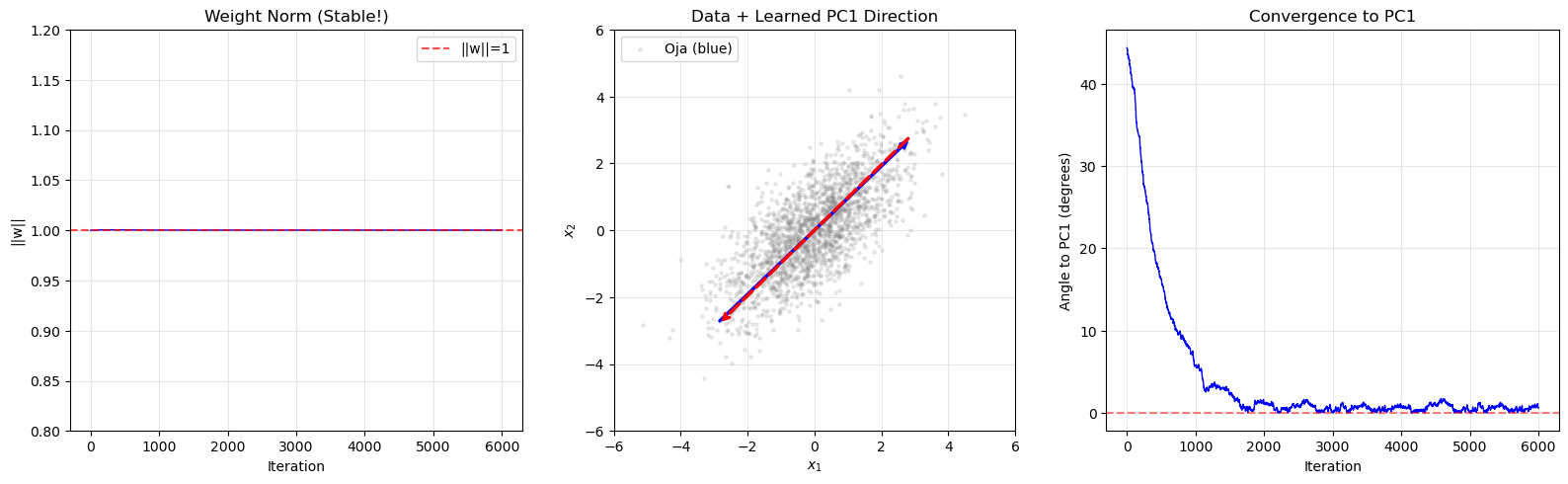
Show code cell source
# 3-panel visualization: Oja's rule convergence
import numpy as np
import matplotlib.pyplot as plt

fig, axes = plt.subplots(1, 3, figsize=(16, 5))

# Panel 1: Weight norm over time
axes[0].plot(oja_norms, color='blue', linewidth=1)
axes[0].axhline(y=1.0, color='red', linestyle='--', label='||w||=1', alpha=0.7)
axes[0].set_xlabel('Iteration')
axes[0].set_ylabel('||w||')
axes[0].set_title('Weight Norm (Stable!)')
axes[0].legend()
axes[0].grid(True, alpha=0.3)
axes[0].set_ylim(0.8, 1.2)

# Panel 2: Data with learned direction
axes[1].scatter(X[:, 0], X[:, 1], alpha=0.15, s=5, color='gray')
w_final = w_oja / np.linalg.norm(w_oja)
scale = 4
axes[1].annotate('', xy=w_final*scale, xytext=-w_final*scale,
                 arrowprops=dict(arrowstyle='->', color='blue', lw=2.5))
axes[1].annotate('', xy=pc1_true*scale, xytext=-pc1_true*scale,
                 arrowprops=dict(arrowstyle='->', color='red', lw=2.5, linestyle='--'))
axes[1].set_xlabel('$x_1$')
axes[1].set_ylabel('$x_2$')
axes[1].set_title('Data + Learned PC1 Direction')
axes[1].set_aspect('equal')
axes[1].set_xlim(-6, 6)
axes[1].set_ylim(-6, 6)
axes[1].legend(['Oja (blue)', 'True PC1 (red)'], loc='upper left')
axes[1].grid(True, alpha=0.3)

# Panel 3: Angle to true PC1 over time
axes[2].plot(oja_angles, color='blue', linewidth=1)
axes[2].axhline(y=0, color='red', linestyle='--', alpha=0.5)
axes[2].set_xlabel('Iteration')
axes[2].set_ylabel('Angle to PC1 (degrees)')
axes[2].set_title('Convergence to PC1')
axes[2].grid(True, alpha=0.3)

plt.tight_layout()
plt.savefig('oja_convergence.png', dpi=150, bbox_inches='tight')
plt.show()
Eigenvector Convergence Visualization#
The following animation-style plot shows the weight vector rotating toward the first principal component over training iterations, superimposed on the 2D data cloud.
Show code cell source
import numpy as np
import matplotlib.pyplot as plt

np.random.seed(42)

# Generate 2D correlated data
n_samples = 2000
angle = np.pi / 4
R = np.array([[np.cos(angle), -np.sin(angle)],
              [np.sin(angle),  np.cos(angle)]])
C_true = R @ np.diag([3.0, 0.5]) @ R.T
X = np.random.multivariate_normal([0, 0], C_true, n_samples)

# True PC1
evals, evecs = np.linalg.eigh(np.cov(X.T))
pc1 = evecs[:, np.argmax(evals)]

# Run Oja's rule and capture snapshots
eta = 0.001
w = np.array([0.0, 1.0])  # start pointing "up" (away from PC1)
w = w / np.linalg.norm(w)

# Capture snapshots at specific iterations
snapshot_iters = [0, 10, 50, 200, 500, 1000, 2000, 4000, 6000]
snapshots = {0: w.copy()}
iteration = 0

for epoch in range(3):
    for i in range(n_samples):
        x = X[i]
        y = w @ x
        w = w + eta * (y * x - y**2 * w)
        iteration += 1
        if iteration in snapshot_iters:
            snapshots[iteration] = w.copy()

# Create the convergence visualization
fig, ax = plt.subplots(figsize=(10, 6))

# Plot data cloud
ax.scatter(X[:, 0], X[:, 1], alpha=0.1, s=3, color='lightgray', zorder=1)

# Plot true PC1 and PC2
pc2 = evecs[:, np.argmin(evals)]
ax.annotate('', xy=pc1*5, xytext=-pc1*5,
            arrowprops=dict(arrowstyle='->', color='red', lw=3, linestyle='--'),
            zorder=5)
ax.annotate('PC1 (target)', xy=pc1*4.5, fontsize=11, color='red',
            fontweight='bold', zorder=5)

# Plot weight vector snapshots with colormap
cmap = plt.cm.viridis
sorted_iters = sorted(snapshots.keys())
n_snaps = len(sorted_iters)

for j, it in enumerate(sorted_iters):
    w_snap = snapshots[it]
    w_dir = w_snap / np.linalg.norm(w_snap)
    color = cmap(j / max(n_snaps - 1, 1))
    scale = 3.5 + 0.5 * j / n_snaps  # slightly growing arrow
    ax.annotate('', xy=w_dir * scale, xytext=[0, 0],
                arrowprops=dict(arrowstyle='->', color=color, lw=2.5),
                zorder=10)
    ax.annotate(f't={it}', xy=w_dir * (scale + 0.3),
                fontsize=8, color=color, zorder=10)

# Draw the unit circle for reference
theta_circle = np.linspace(0, 2*np.pi, 200)
ax.plot(3.5*np.cos(theta_circle), 3.5*np.sin(theta_circle),
        'k--', alpha=0.15, linewidth=1)

ax.set_xlabel('$x_1$', fontsize=12)
ax.set_ylabel('$x_2$', fontsize=12)
ax.set_title("Oja's Rule: Weight Vector Rotating Toward PC1\n"
             "(color: early=dark, late=yellow)", fontsize=13)
ax.set_aspect('equal')
ax.set_xlim(-6, 6)
ax.set_ylim(-6, 6)
ax.grid(True, alpha=0.3)

plt.tight_layout()
plt.show()

print("The weight vector (colored arrows) rotates from its initial direction")
print("toward the leading eigenvector (red dashed arrow) over training.")
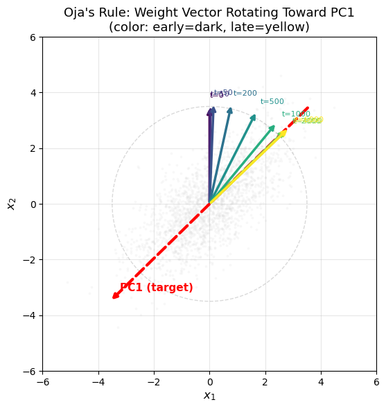
The weight vector (colored arrows) rotates from its initial direction
toward the leading eigenvector (red dashed arrow) over training.
Side-by-Side: Exact PCA vs Online Oja#
The following comparison demonstrates that Oja’s online rule converges to the same result as exact (batch) PCA computed via eigendecomposition, using a higher-dimensional dataset.
Show code cell source
import numpy as np
import matplotlib.pyplot as plt

np.random.seed(42)

# Generate 5D correlated data with known principal components
n_dim = 5
n_samples = 5000

# Create a covariance matrix with distinct eigenvalues
true_eigenvalues = np.array([5.0, 3.0, 1.5, 0.5, 0.1])
# Random orthogonal matrix for eigenvectors
Q, _ = np.linalg.qr(np.random.randn(n_dim, n_dim))
C_true = Q @ np.diag(true_eigenvalues) @ Q.T

X = np.random.multivariate_normal(np.zeros(n_dim), C_true, n_samples)

# --- Exact PCA ---
C_sample = np.cov(X.T)
evals_exact, evecs_exact = np.linalg.eigh(C_sample)
idx_sort = np.argsort(-evals_exact)
evals_exact = evals_exact[idx_sort]
evecs_exact = evecs_exact[:, idx_sort]
pc1_exact = evecs_exact[:, 0]

# --- Oja's Rule (online) ---
eta = 0.0005
w_oja = np.random.randn(n_dim)
w_oja = w_oja / np.linalg.norm(w_oja)

oja_norms = [np.linalg.norm(w_oja)]
oja_angles = []
cos_a = np.clip(np.abs(w_oja @ pc1_exact) / np.linalg.norm(w_oja), -1, 1)
oja_angles.append(np.degrees(np.arccos(cos_a)))

for epoch in range(5):
    for i in range(n_samples):
        x = X[i]
        y = w_oja @ x
        w_oja = w_oja + eta * (y * x - y**2 * w_oja)
        if i % 50 == 0:
            oja_norms.append(np.linalg.norm(w_oja))
            cos_a = np.clip(np.abs(w_oja @ pc1_exact) / np.linalg.norm(w_oja), -1, 1)
            oja_angles.append(np.degrees(np.arccos(cos_a)))

w_oja_final = w_oja / np.linalg.norm(w_oja)

# --- Projection comparison ---
proj_exact = X @ pc1_exact
proj_oja = X @ w_oja_final

# Align sign (PC direction is arbitrary up to sign)
if np.corrcoef(proj_exact, proj_oja)[0, 1] < 0:
    proj_oja = -proj_oja
    w_oja_final = -w_oja_final

# Visualization
fig, axes = plt.subplots(1, 3, figsize=(16, 5))

# Panel 1: Component comparison
x_pos = np.arange(n_dim)
width = 0.35
axes[0].bar(x_pos - width/2, pc1_exact, width, label='Exact PCA', color='#E91E63', alpha=0.8)
axes[0].bar(x_pos + width/2, w_oja_final, width, label='Oja (online)', color='#2196F3', alpha=0.8)
axes[0].set_xlabel('Component index', fontsize=11)
axes[0].set_ylabel('Weight value', fontsize=11)
axes[0].set_title('PC1 Components: Exact vs Oja', fontsize=12)
axes[0].set_xticks(x_pos)
axes[0].legend(fontsize=10)
axes[0].grid(True, alpha=0.3, axis='y')

# Panel 2: Projection scatter
axes[1].scatter(proj_exact, proj_oja, alpha=0.1, s=3, color='steelblue')
lim = max(np.abs(proj_exact).max(), np.abs(proj_oja).max()) * 1.1
axes[1].plot([-lim, lim], [-lim, lim], 'r--', linewidth=1, label='y = x')
axes[1].set_xlabel('Exact PCA projection', fontsize=11)
axes[1].set_ylabel('Oja projection', fontsize=11)
axes[1].set_title(f'Projection Comparison (r = {np.corrcoef(proj_exact, proj_oja)[0,1]:.6f})',
                  fontsize=12)
axes[1].set_aspect('equal')
axes[1].legend(fontsize=10)
axes[1].grid(True, alpha=0.3)

# Panel 3: Convergence angle over time
axes[2].plot(oja_angles, color='#2196F3', linewidth=1.5)
axes[2].axhline(y=0, color='red', linestyle='--', alpha=0.5)
axes[2].set_xlabel('Iteration (x50)', fontsize=11)
axes[2].set_ylabel('Angle to true PC1 (degrees)', fontsize=11)
axes[2].set_title('Oja Convergence in 5D', fontsize=12)
axes[2].grid(True, alpha=0.3)

plt.suptitle('Exact PCA vs Online Oja\'s Rule on 5D Data', fontsize=14, fontweight='bold', y=1.02)
plt.tight_layout()
plt.show()

print(f"Exact PC1:  {pc1_exact}")
print(f"Oja PC1:    {w_oja_final}")
print(f"Cosine similarity: {np.abs(pc1_exact @ w_oja_final):.8f}")
print(f"Oja final norm: {np.linalg.norm(w_oja):.6f}")
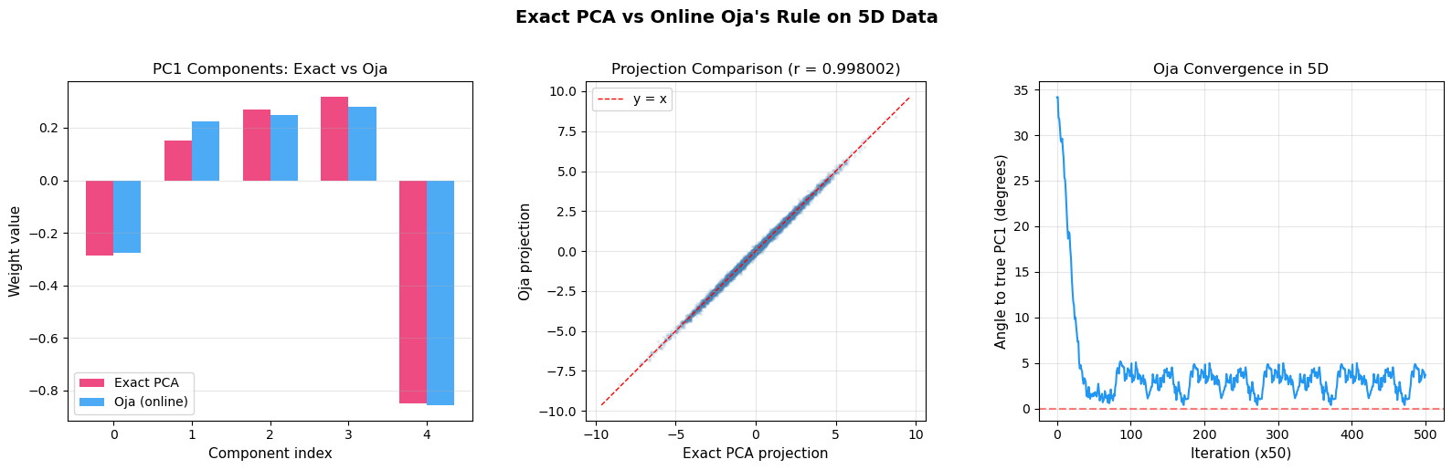
Exact PC1:  [-0.28676795  0.151474    0.26804922  0.31720183 -0.84991316]
Oja PC1:    [-0.27703178  0.2240857   0.24808732  0.28068937 -0.85598198]
Cosine similarity: 0.99643214
Oja final norm: 1.000575
Weight Norm Stability: Oja vs Pure Hebb#
This visualization directly compares how the weight norm evolves under Oja’s rule (stabilized at \(\|\mathbf{w}\| \approx 1\)) versus pure Hebbian learning (diverges exponentially).
Show code cell source
import numpy as np
import matplotlib.pyplot as plt

np.random.seed(42)

# Generate 2D correlated data
n_samples = 2000
angle = np.pi / 4
R = np.array([[np.cos(angle), -np.sin(angle)],
              [np.sin(angle),  np.cos(angle)]])
C_true = R @ np.diag([3.0, 0.5]) @ R.T
X = np.random.multivariate_normal([0, 0], C_true, n_samples)

eta = 0.001
w_init = np.array([0.5, 0.5])
w_init = w_init / np.linalg.norm(w_init)

# --- Pure Hebb ---
w_hebb = w_init.copy()
hebb_norms = [np.linalg.norm(w_hebb)]

for epoch in range(3):
    for i in range(n_samples):
        x = X[i]
        y = w_hebb @ x
        w_hebb = w_hebb + eta * y * x
        hebb_norms.append(np.linalg.norm(w_hebb))

# --- Oja ---
w_oja = w_init.copy()
oja_norms_compare = [np.linalg.norm(w_oja)]

for epoch in range(3):
    for i in range(n_samples):
        x = X[i]
        y = w_oja @ x
        w_oja = w_oja + eta * (y * x - y**2 * w_oja)
        oja_norms_compare.append(np.linalg.norm(w_oja))

# --- Hebb + explicit normalization ---
w_hebb_norm = w_init.copy()
hebb_norm_norms = [np.linalg.norm(w_hebb_norm)]

for epoch in range(3):
    for i in range(n_samples):
        x = X[i]
        y = w_hebb_norm @ x
        w_hebb_norm = w_hebb_norm + eta * y * x
        w_hebb_norm = w_hebb_norm / np.linalg.norm(w_hebb_norm)  # explicit normalize
        hebb_norm_norms.append(np.linalg.norm(w_hebb_norm))

# Visualization
fig, axes = plt.subplots(1, 2, figsize=(14, 5))

iterations = np.arange(len(hebb_norms))

# Panel 1: Log scale comparison
axes[0].plot(iterations, hebb_norms, color='red', linewidth=2, label='Pure Hebb (diverges)')
axes[0].plot(iterations, oja_norms_compare, color='blue', linewidth=2, label="Oja's Rule (stable)")
axes[0].plot(iterations, hebb_norm_norms, color='green', linewidth=2,
             linestyle='--', label='Hebb + normalize')
axes[0].set_yscale('log')
axes[0].set_xlabel('Iteration', fontsize=12)
axes[0].set_ylabel('$||\\mathbf{w}||$ (log scale)', fontsize=12)
axes[0].set_title('Weight Norm: Three Learning Rules', fontsize=13)
axes[0].legend(fontsize=11)
axes[0].grid(True, alpha=0.3)

# Panel 2: Zoomed in on Oja near ||w||=1
axes[1].plot(iterations, oja_norms_compare, color='blue', linewidth=1.5, label="Oja's Rule")
axes[1].axhline(y=1.0, color='red', linestyle='--', linewidth=1.5, label='$||w|| = 1$', alpha=0.7)
axes[1].set_xlabel('Iteration', fontsize=12)
axes[1].set_ylabel('$||\\mathbf{w}||$', fontsize=12)
axes[1].set_title("Oja's Rule: Norm Stabilizes at 1", fontsize=13)
axes[1].set_ylim(0.85, 1.15)
axes[1].legend(fontsize=11)
axes[1].grid(True, alpha=0.3)

plt.suptitle('Weight Norm Over Time: Why Oja Fixes Hebbian Instability',
             fontsize=14, fontweight='bold', y=1.02)
plt.tight_layout()
plt.show()

print(f"Final norms: Pure Hebb = {hebb_norms[-1]:.2f}, Oja = {oja_norms_compare[-1]:.4f}, "
      f"Hebb+normalize = {hebb_norm_norms[-1]:.4f}")
print("\nKey insight: Oja's rule achieves the same effect as 'Hebb + normalize'")
print("but through a single elegant update rule with no explicit normalization step.")
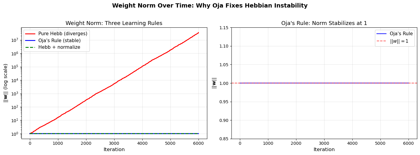
Final norms: Pure Hebb = 35585443.36, Oja = 1.0001, Hebb+normalize = 1.0000

Key insight: Oja's rule achieves the same effect as 'Hebb + normalize'
but through a single elegant update rule with no explicit normalization step.
13.4 Sanger’s Generalized Hebbian Algorithm (GHA)#
Oja’s rule extracts only the first principal component. To extract multiple components, Sanger (1989) proposed the Generalized Hebbian Algorithm (GHA).
Setup#
Consider \(p\) output neurons with weight vectors \(\mathbf{w}_1, \ldots, \mathbf{w}_p\), arranged in a weight matrix \(\mathbf{W} \in \mathbb{R}^{p \times n}\) where row \(j\) is \(\mathbf{w}_j^\top\).
Outputs: \(y_j = \mathbf{w}_j^\top \mathbf{x}\) for \(j = 1, \ldots, p\).
Sanger’s Rule#
In matrix form, using \(\text{LT}(\cdot)\) to denote the lower-triangular part (including diagonal):
Key Idea#
The first neuron (\(j=1\)) follows Oja’s rule exactly: \(\Delta \mathbf{w}_1 = \eta(y_1 \mathbf{x} - y_1^2 \mathbf{w}_1)\)
Each subsequent neuron effectively learns from a deflated input, with the projections onto previously extracted components removed.
Result: \(\mathbf{w}_j \to \pm \mathbf{e}_j\) (the \(j\)-th principal component).
Convergence#
Under appropriate conditions on the learning rate, GHA converges to the first \(p\) principal components in order: \(\mathbf{w}_1 \to \pm\mathbf{e}_1\), \(\mathbf{w}_2 \to \pm\mathbf{e}_2\), etc.
Show code cell source
import numpy as np
import matplotlib.pyplot as plt
# Side-by-side comparison: Basic Hebb vs Oja's Rule
np.random.seed(123)
# Generate correlated 2D data
n_samples = 2000
angle = np.pi / 3
R = np.array([[np.cos(angle), -np.sin(angle)],
[np.sin(angle), np.cos(angle)]])
C_true = R @ np.diag([3.0, 0.5]) @ R.T
X = np.random.multivariate_normal([0, 0], C_true, n_samples)
# True PC1
evals, evecs = np.linalg.eigh(np.cov(X.T))
pc1 = evecs[:, np.argmax(evals)]
eta = 0.001
w_init = np.array([0.5, 0.5])
w_init = w_init / np.linalg.norm(w_init)
# Basic Hebb
w_hebb = w_init.copy()
hebb_norms = [np.linalg.norm(w_hebb)]
hebb_angles = []
cos_a = np.clip(np.abs(w_hebb @ pc1) / np.linalg.norm(w_hebb), -1, 1)
hebb_angles.append(np.degrees(np.arccos(cos_a)))
for epoch in range(3):
for i in range(n_samples):
x = X[i]
y = w_hebb @ x
w_hebb = w_hebb + eta * y * x
hebb_norms.append(np.linalg.norm(w_hebb))
cos_a = np.clip(np.abs(w_hebb @ pc1) / np.linalg.norm(w_hebb), -1, 1)
hebb_angles.append(np.degrees(np.arccos(cos_a)))
# Oja
w_oja = w_init.copy()
oja_norms2 = [np.linalg.norm(w_oja)]
oja_angles2 = []
cos_a = np.clip(np.abs(w_oja @ pc1) / np.linalg.norm(w_oja), -1, 1)
oja_angles2.append(np.degrees(np.arccos(cos_a)))
for epoch in range(3):
for i in range(n_samples):
x = X[i]
y = w_oja @ x
w_oja = w_oja + eta * (y * x - y**2 * w_oja)
oja_norms2.append(np.linalg.norm(w_oja))
cos_a = np.clip(np.abs(w_oja @ pc1) / np.linalg.norm(w_oja), -1, 1)
oja_angles2.append(np.degrees(np.arccos(cos_a)))
# Plot comparison
fig, axes = plt.subplots(1, 3, figsize=(16, 5))
# Norm comparison
axes[0].plot(hebb_norms, label='Basic Hebb', color='red', alpha=0.8)
axes[0].plot(oja_norms2, label="Oja's Rule", color='blue', alpha=0.8)
axes[0].set_xlabel('Iteration')
axes[0].set_ylabel('||w||')
axes[0].set_title('Weight Norm Comparison')
axes[0].set_yscale('log')
axes[0].legend()
axes[0].grid(True, alpha=0.3)
# Data with both learned directions
axes[1].scatter(X[:, 0], X[:, 1], alpha=0.15, s=5, color='gray')
s = 4
# Hebb direction (normalized)
w_h_dir = w_hebb / np.linalg.norm(w_hebb)
axes[1].annotate('', xy=w_h_dir*s, xytext=[0,0],
arrowprops=dict(arrowstyle='->', color='red', lw=2.5))
# Oja direction
w_o_dir = w_oja / np.linalg.norm(w_oja)
axes[1].annotate('', xy=w_o_dir*s, xytext=[0,0],
arrowprops=dict(arrowstyle='->', color='blue', lw=2.5))
# True PC1
axes[1].annotate('', xy=pc1*s, xytext=[0,0],
arrowprops=dict(arrowstyle='->', color='green', lw=2.5, linestyle='--'))
axes[1].set_xlabel('$x_1$')
axes[1].set_ylabel('$x_2$')
axes[1].set_title('Learned Directions')
axes[1].legend(['Hebb', 'Oja', 'True PC1'], loc='upper left')
axes[1].set_aspect('equal')
axes[1].set_xlim(-6, 6)
axes[1].set_ylim(-6, 6)
axes[1].grid(True, alpha=0.3)
# Angle comparison
axes[2].plot(hebb_angles, label='Basic Hebb', color='red', alpha=0.8)
axes[2].plot(oja_angles2, label="Oja's Rule", color='blue', alpha=0.8)
axes[2].axhline(y=0, color='gray', linestyle='--', alpha=0.5)
axes[2].set_xlabel('Iteration')
axes[2].set_ylabel('Angle to PC1 (degrees)')
axes[2].set_title('Direction Convergence')
axes[2].legend()
axes[2].grid(True, alpha=0.3)
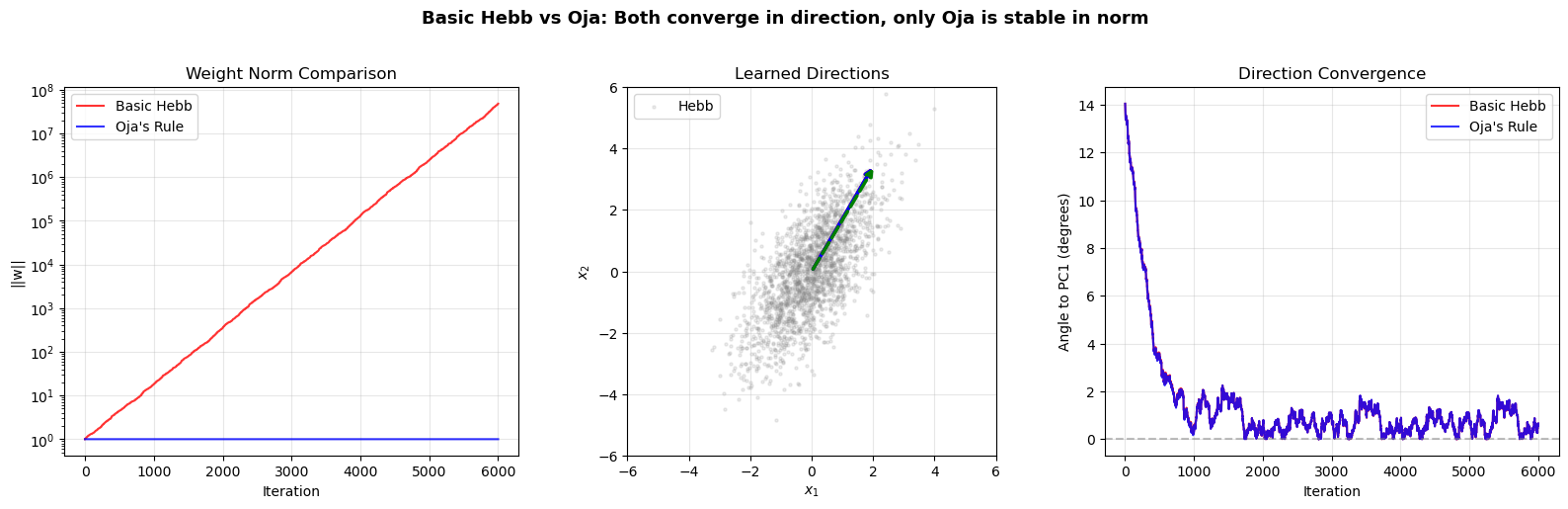
plt.suptitle('Basic Hebb vs Oja: Both converge in direction, only Oja is stable in norm',
fontsize=13, fontweight='bold', y=1.02)
plt.tight_layout()
plt.savefig('hebb_vs_oja.png', dpi=150, bbox_inches='tight')
plt.show()
Exercises#
Exercise 13.1. Implement Sanger’s GHA to extract the first 3 principal components of a
5-dimensional dataset. Compare the extracted components with those from numpy.linalg.eigh.
Exercise 13.2. Apply Oja’s rule to the Iris dataset (4 features). Compare the learned
direction with the output of sklearn.decomposition.PCA. Visualize the data projected onto
the leading eigenvector of \(\mathbf{C}\) (for centered data, the first principal component).
Exercise 13.3. Investigate the effect of the learning rate \(\eta\) on Oja’s rule. For various values of \(\eta\), plot (a) the convergence speed (iterations to reach angle < 1 degree) and (b) whether the norm remains stable. What happens for very large \(\eta\)?
Exercise 13.4. Prove that the equilibrium points of Oja’s rule on the unit sphere are exactly the eigenvectors of \(\mathbf{C}\). (Hint: Set \(d\mathbf{w}/dt = 0\) with the constraint \(\|\mathbf{w}\| = 1\).)
Exercise 13.5. Implement a mini-batch version of Oja’s rule where the weight update averages over a batch of \(B\) samples. Compare convergence for \(B = 1, 10, 50, 200\).