Chapter 21: From Pixels to Features

Chapter 21: From Pixels to Features#

In the previous chapters, we built fully connected multilayer networks capable of approximating any continuous function. These networks are powerful in theory, but when we turn to image data, their architecture reveals a critical weakness: every input pixel connects to every hidden neuron, creating an explosion of parameters that makes learning slow, memory-hungry, and prone to overfitting.

This chapter motivates the transition from fully connected networks to convolutional neural networks (CNNs) by identifying the structural assumptions that make image processing fundamentally different from generic function approximation. We will see how three elegant ideas—weight sharing, local receptive fields, and translation equivariance—reduce the parameter count by orders of magnitude while encoding the spatial structure of visual data directly into the network architecture.

1. The Curse of Full Connectivity#

Consider the simplest image classification task: recognizing handwritten digits from \(28 \times 28\) grayscale images (the MNIST dataset). Each image has \(28 \times 28 = 784\) pixels, so the input layer has 784 neurons.

In a fully connected network with a single hidden layer of 100 neurons, the first layer alone requires:

\[784 \times 100 + 100 = 78{,}500 \text{ parameters}\]

This is already substantial for a tiny \(28 \times 28\) image. What happens with realistic image sizes?

import numpy as np

# Parameter counts for fully connected first layer (input -> 100 hidden neurons)
image_sizes = {
    'MNIST (28x28)':        (28, 28, 1),
    'CIFAR-10 (32x32x3)':   (32, 32, 3),
    'ImageNet (224x224x3)':  (224, 224, 3),
    'HD photo (1920x1080x3)':(1920, 1080, 3),
}

hidden_neurons = 100

print("Fully connected layer: input -> 100 hidden neurons")
print("=" * 60)
for name, (h, w, c) in image_sizes.items():
    input_dim = h * w * c
    fc_params = input_dim * hidden_neurons + hidden_neurons  # weights + biases
    print(f"{name:30s}  input_dim = {input_dim:>10,d}  params = {fc_params:>15,d}")

# Compare with a CNN: 16 filters of size 3x3 on a single-channel input
print("\nConvolutional layer: 16 filters of 3x3 on 1-channel input")
print("=" * 60)
num_filters = 16
kernel_size = 3
in_channels = 1
conv_params = num_filters * (in_channels * kernel_size * kernel_size + 1)  # weights + biases
print(f"Parameters (independent of image size): {conv_params}")
print(f"\nRatio for MNIST: {78_500 / conv_params:.0f}x fewer parameters with convolution")

Fully connected layer: input -> 100 hidden neurons
============================================================
MNIST (28x28)                   input_dim =        784  params =          78,500
CIFAR-10 (32x32x3)              input_dim =      3,072  params =         307,300
ImageNet (224x224x3)            input_dim =    150,528  params =      15,052,900
HD photo (1920x1080x3)          input_dim =  6,220,800  params =     622,080,100

Convolutional layer: 16 filters of 3x3 on 1-channel input
============================================================
Parameters (independent of image size): 160

Ratio for MNIST: 491x fewer parameters with convolution

The numbers are striking. A single fully connected layer on a modest \(224 \times 224 \times 3\) colour image requires over 15 million parameters—before we even add a second layer. Meanwhile, a convolutional layer with 16 filters of size \(3 \times 3\) uses only 160 parameters, regardless of the input image size.

The Core Problem

Fully connected layers treat every pixel as an independent feature with no spatial relationship to its neighbours. This wastes capacity on learning redundant patterns and demands enormous amounts of training data to generalize.

The solution is to design an architecture that respects the spatial structure of images. This is precisely what convolutional neural networks do.

2. Three Key Ideas#

Convolutional neural networks are built on three principles that exploit the structure of visual data.

2.1 Local Receptive Fields#

Definition (Local Receptive Field)

A local receptive field is a small, contiguous region of the input (e.g., a \(3 \times 3\) or \(5 \times 5\) patch) to which a single hidden neuron is connected. Instead of seeing the entire image, each neuron receives input only from a spatially localized neighbourhood.

This reflects a fundamental property of natural images: nearby pixels are strongly correlated (they tend to belong to the same object, edge, or texture), while distant pixels carry largely independent information. A neuron responsible for detecting a vertical edge needs only a small local patch to do its job.

2.3 Translation Equivariance#

Definition (Translation Equivariance)

A function \(f\) is translation equivariant if shifting the input causes an identical shift in the output:

\[f(\text{shift}(\bx)) = \text{shift}(f(\bx))\]

Convolution is inherently translation equivariant: if a cat’s ear appears 10 pixels to the right, the corresponding feature map activation also shifts 10 pixels to the right.

This is distinct from translation invariance (the output does not change at all when the input is shifted). Pure convolution is equivariant, not invariant. Invariance is typically achieved later in the pipeline through pooling operations.

Equivariance vs. Invariance

Equivariance: “If the input moves, the output moves with it.” (Convolution)
Invariance: “If the input moves, the output stays the same.” (Global average pooling, classification head)

A CNN typically starts with equivariant layers (convolutions) and progressively introduces invariance (pooling, global averaging) so that the final class prediction is insensitive to the object’s position.

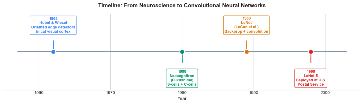
3. Historical Context#

The ideas behind convolutional networks did not appear in a vacuum. They emerged from a rich interaction between neuroscience and computer science spanning several decades.

Hubel & Wiesel (1962): The Neuroscience Foundation#

David Hubel and Torsten Wiesel performed groundbreaking experiments on the cat visual cortex, discovering that individual neurons respond to oriented edges at specific positions in the visual field. They identified two types of cells:

Simple cells: respond to edges of a particular orientation at a specific location (analogous to convolutional filters).
Complex cells: respond to edges of a particular orientation regardless of exact position (analogous to pooling).

Their work earned the Nobel Prize in Physiology or Medicine (1981) and directly inspired the hierarchical feature extraction architecture of CNNs.

The Neocognitron (Fukushima, 1980)#

Kunihiko Fukushima built the Neocognitron, a hierarchical neural network explicitly modeled on Hubel and Wiesel’s findings. It introduced:

Alternating layers of S-cells (simple, feature-extracting) and C-cells (complex, position-invariant).
Local receptive fields and weight sharing.
Training via a self-organizing (unsupervised) rule rather than backpropagation.

The Neocognitron was the first neural architecture to successfully recognize handwritten characters with some positional invariance.

LeNet (LeCun et al., 1989–1998)#

Yann LeCun combined the architectural ideas of the Neocognitron with backpropagation (Chapter 16) to create LeNet, the first CNN trained end-to-end with gradient descent. Key milestones:

1989: LeCun et al. applied backpropagation to a convolutional network for handwritten zip code recognition.
1998: LeNet-5, the mature architecture, was deployed by the U.S. Postal Service for reading handwritten digits on mail, processing millions of checks.

LeNet-5 established the modern CNN template: convolutional layers \(\to\) pooling layers \(\to\) fully connected layers.

../_images/ce5b1286c5e4c29ab9c6f49e30b54bb7ddcca9e1ae05141efb277a67f3b1eedf.png

4. The CNN Pipeline#

A typical convolutional neural network processes an image through a sequence of distinct stages:

Convolutional layers extract local features (edges, textures, shapes) by sliding learned filters across the input.
Activation functions (typically ReLU) introduce nonlinearity after each convolution.
Pooling layers reduce spatial dimensions, introducing a degree of translation invariance.
These three operations are repeated in multiple stages, with each stage extracting increasingly abstract features.
Flattening converts the final 2D feature maps into a 1D vector.
Fully connected (dense) layers combine the extracted features for classification.
Softmax produces a probability distribution over classes.

The following diagram illustrates this pipeline:

Show code cell source Hide code cell source

import matplotlib.pyplot as plt
import matplotlib.patches as mpatches
import numpy as np

plt.style.use('seaborn-v0_8-whitegrid')

fig, ax = plt.subplots(figsize=(14, 4))

# Pipeline stages
stages = [
    ('Input\nImage',       '#64748b', (0.8, 1.6)),
    ('Conv',               '#3b82f6', (0.7, 1.4)),
    ('ReLU',               '#2563eb', (0.6, 1.2)),
    ('Pool',               '#059669', (0.5, 1.0)),
    ('Conv',               '#3b82f6', (0.5, 1.0)),
    ('ReLU',               '#2563eb', (0.45, 0.9)),
    ('Pool',               '#059669', (0.4, 0.8)),
    ('Flatten',            '#d97706', (0.15, 1.4)),
    ('Dense',              '#dc2626', (0.15, 1.2)),
    ('Softmax',            '#7c3aed', (0.15, 1.0)),
]

x_pos = 0.5
x_positions = []
gap = 0.15

for i, (label, color, (w, h)) in enumerate(stages):
    x_positions.append(x_pos)
    rect = mpatches.FancyBboxPatch(
        (x_pos - w/2, -h/2), w, h,
        boxstyle=mpatches.BoxStyle('Round', pad=0.05),
        facecolor=color, edgecolor='white', linewidth=2, alpha=0.85
    )
    ax.add_patch(rect)
    ax.text(x_pos, 0, label, ha='center', va='center',
            fontsize=9, fontweight='bold', color='white')
    
    # Arrow to next stage
    if i < len(stages) - 1:
        next_w = stages[i+1][2][0]
        arrow_start = x_pos + w/2 + 0.02
        next_x = x_pos + w/2 + gap + next_w/2
        arrow_end = next_x - next_w/2 - 0.02
        ax.annotate('', xy=(arrow_end, 0), xytext=(arrow_start, 0),
                    arrowprops=dict(arrowstyle='->', color='#94a3b8',
                                   lw=1.5, connectionstyle='arc3,rad=0'))
    
    x_pos += w/2 + gap + (stages[i+1][2][0]/2 if i < len(stages)-1 else 0)

# Bracket labels for feature extraction vs classification
ax.annotate('', xy=(x_positions[0] - 0.4, -1.15), xytext=(x_positions[6] + 0.4, -1.15),
            arrowprops=dict(arrowstyle='-', color='#3b82f6', lw=1.5))
ax.text((x_positions[0] + x_positions[6])/2, -1.35,
        'Feature Extraction', ha='center', fontsize=10, color='#3b82f6', fontstyle='italic')

ax.annotate('', xy=(x_positions[7] - 0.1, -1.15), xytext=(x_positions[9] + 0.1, -1.15),
            arrowprops=dict(arrowstyle='-', color='#dc2626', lw=1.5))
ax.text((x_positions[7] + x_positions[9])/2, -1.35,
        'Classification', ha='center', fontsize=10, color='#dc2626', fontstyle='italic')

ax.set_xlim(-0.2, x_pos + 0.5)
ax.set_ylim(-1.8, 1.3)
ax.set_aspect('equal')
ax.axis('off')
ax.set_title('The CNN Pipeline', fontsize=14, fontweight='bold', pad=15)

plt.tight_layout()
plt.show()

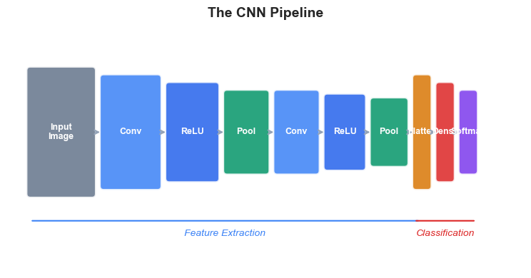
../_images/7bbfc1a110f139c7b65b2d6ed9b372caa712ad37013f744e2bf55cd623f9b461.png

Key insight: The early convolutional layers detect simple, local features (edges, corners). As we go deeper, the receptive field of each neuron grows, and the network learns to combine low-level features into higher-level representations (textures \(\to\) parts \(\to\) objects). This hierarchical feature extraction mirrors the organization of the primate visual cortex discovered by Hubel and Wiesel.

In the next chapters, we will build each of these components from scratch:

Chapter	Component	Key Concept
22	Convolution	Sliding filter, cross-correlation, feature maps
23	Pooling & Architecture	Max pooling, stride, padding, LeNet-5
24	CNN Backpropagation	Gradients through conv and pool layers

5. Exercises#

Exercise 21.1: Parameter Counting#

A colour image of size \(64 \times 64 \times 3\) is fed into a fully connected layer with 256 hidden neurons.

(a) How many parameters (weights + biases) does this layer have?

(b) Now consider a convolutional layer with 32 filters of size \(5 \times 5\), applied to the same \(64 \times 64 \times 3\) input. How many parameters does this layer have?

Exercise 21.2: Equivariance vs. Invariance#

Let \(f\) be a function mapping images to feature maps, and let \(T_\delta\) denote a spatial translation by \(\delta\) pixels.

(a) Write the mathematical condition for \(f\) to be translation equivariant.

(b) Write the mathematical condition for \(f\) to be translation invariant.

(d) Give an example of a function that is translation invariant. Why is pure invariance undesirable in the early layers of a vision network?

Exercise 21.3: Receptive Field Growth#

Consider a network with two consecutive \(3 \times 3\) convolutional layers (stride 1, no padding).

(a) What is the effective receptive field of a single neuron in the second convolutional layer’s output? That is, how large a region of the original input does it depend on?

(b) Generalize: if we stack \(L\) convolutional layers, each with kernel size \(K \times K\) (stride 1, no padding), what is the effective receptive field size?

© How many \(3 \times 3\) layers would we need to achieve the same receptive field as a single \(7 \times 7\) filter? Which approach uses fewer parameters (assuming the same number of input and output channels)?

Exercise 21.4: Why Not Fully Connected?#

Suppose you train a fully connected network on \(28 \times 28\) images of the digit “7”, and it learns to recognize the digit when it appears in the centre of the image.

(a) Will the network correctly recognize a “7” shifted 5 pixels to the right? Explain why or why not, referring to the structure of the weight matrix.

(b) How does a convolutional network handle this same scenario differently?

Exercise 21.5: Biological Analogy#

Hubel and Wiesel identified simple cells and complex cells in the cat visual cortex.

(a) Which CNN component is analogous to simple cells? Which is analogous to complex cells?

(b) In what important ways does the analogy break down? Consider at least two differences between biological vision and CNNs.

6. Summary and Key Takeaways#

Fully connected networks suffer from a parameter explosion on image data, requiring millions of weights even for modest image sizes.
Convolutional neural networks solve this through three key ideas:
- Local receptive fields: each neuron sees only a small patch.
- Weight sharing: the same filter is applied everywhere.
- Translation equivariance: shifting the input shifts the output.
The CNN architecture was inspired by Hubel & Wiesel’s neuroscience discoveries (1962) and developed through Fukushima’s Neocognitron (1980) and LeCun’s LeNet (1989–1998).
The standard CNN pipeline consists of: Convolution \(\to\) ReLU \(\to\) Pooling (repeated), followed by Flatten \(\to\) Dense \(\to\) Softmax.

7. References#

D. H. Hubel and T. N. Wiesel, “Receptive fields, binocular interaction and functional architecture in the cat’s visual cortex,” The Journal of Physiology, vol. 160, no. 1, pp. 106–154, 1962.
K. Fukushima, “Neocognitron: A self-organizing neural network model for a mechanism of pattern recognition unaffected by shift in position,” Biological Cybernetics, vol. 36, no. 4, pp. 193–202, 1980.
Y. LeCun, B. Boser, J. S. Denker, D. Henderson, R. E. Howard, W. Hubbard, and L. D. Jackel, “Backpropagation applied to handwritten zip code recognition,” Neural Computation, vol. 1, no. 4, pp. 541–551, 1989.
Y. LeCun, L. Bottou, Y. Bengio, and P. Haffner, “Gradient-based learning applied to document recognition,” Proceedings of the IEEE, vol. 86, no. 11, pp. 2278–2324, 1998.