Chapter 5: The Perceptron Learning Algorithm

Chapter 5: The Perceptron Learning Algorithm#

Part 2: The Perceptron#

5.1 Introduction: The Key Innovation#

The most revolutionary aspect of Rosenblatt’s perceptron was not the model itself – a single neuron computing a weighted sum passed through a threshold had been considered by McCulloch and Pitts in 1943. The breakthrough was the learning algorithm: a simple iterative procedure that could automatically discover the correct weights from labeled examples.

Before Rosenblatt, building a neural network required a human designer to:

Analyze the problem.
Determine the correct weights and thresholds by hand.
Wire the network accordingly.

After Rosenblatt, the process became:

Collect labeled training examples: \((\mathbf{x}_1, y_1), (\mathbf{x}_2, y_2), \ldots, (\mathbf{x}_m, y_m)\).
Initialize the weights (e.g., to zero).
Run the learning algorithm, which adjusts weights automatically.

This shift from design to learning is the philosophical cornerstone of modern machine learning.

5.2 The Weight Update Rule#

Algorithm (Perceptron Learning Rule)

Given a training example \((\mathbf{x}, y)\) where \(y \in \{0, 1\}\) is the true label and \(\hat{y} = f(\mathbf{x})\) is the predicted label, the perceptron update rule is:

\[\mathbf{w}_{t+1} = \mathbf{w}_t + \eta(y - \hat{y})\mathbf{x}\]

\[b_{t+1} = b_t + \eta(y - \hat{y})\]

where \(\eta > 0\) is the learning rate. The update is applied only when the perceptron makes a misclassification (\(\hat{y} \neq y\)). When the prediction is correct, \((y - \hat{y}) = 0\) and no change occurs.

Case Analysis

Since both \(y\) and \(\hat{y}\) are binary, there are four possibilities:

Case	\(y\)	\(\hat{y}\)	\(y - \hat{y}\)	Action	Geometric Effect
Correct positive	1	1	0	No update	–
Correct negative	0	0	0	No update	–
False negative	1	0	+1	\(\mathbf{w} \leftarrow \mathbf{w} + \eta\mathbf{x}\)	Rotate \(\mathbf{w}\) toward \(\mathbf{x}\)
False positive	0	1	-1	\(\mathbf{w} \leftarrow \mathbf{w} - \eta\mathbf{x}\)	Rotate \(\mathbf{w}\) away from \(\mathbf{x}\)

Tip

Geometric Interpretation of Weight Updates

Think of the weight vector \(\mathbf{w}\) as an arrow pointing toward the “positive” side of the decision boundary. Each update rotates the hyperplane:

False negative (\(y=1\), \(\hat{y}=0\)): The input \(\mathbf{x}\) should be on the positive side but isn’t. Adding \(\eta\mathbf{x}\) to \(\mathbf{w}\) rotates the boundary so that \(\mathbf{w}\) points more toward \(\mathbf{x}\), pulling the positive region to include it.
False positive (\(y=0\), \(\hat{y}=1\)): The input \(\mathbf{x}\) should be on the negative side but isn’t. Subtracting \(\eta\mathbf{x}\) from \(\mathbf{w}\) rotates the boundary away from \(\mathbf{x}\), pushing the positive region away.

Each update is a local correction: it improves classification of the current point without regard for other points. The remarkable fact (proven by the convergence theorem in Chapter 6) is that these local corrections globally converge to a correct solution, provided one exists.

Warning

Important Conditions for the Perceptron Learning Rule

The learning rate \(\eta\) must be strictly positive (\(\eta > 0\)). If \(\eta = 0\), no updates occur and the algorithm cannot learn.
The algorithm is guaranteed to converge only for linearly separable data. If the data is not linearly separable, the algorithm will oscillate indefinitely without finding a solution.
For the step activation function, the value of \(\eta\) does not affect the number of epochs or whether convergence occurs – only the magnitude of the final weights changes. This is a special property of the step function.

Danger

If the training data is NOT linearly separable, the perceptron learning algorithm will loop forever (or until the maximum epoch limit is reached). It will never achieve zero training error, and the decision boundary will oscillate without settling. There is no built-in mechanism to detect this situation – the algorithm simply keeps updating weights indefinitely. This is why the convergence theorem’s assumption of linear separability is critical.

5.3 The Full Algorithm#

Here is the complete perceptron learning algorithm in pseudocode:

Algorithm: Perceptron Learning Algorithm

Input: Training set \(\{(\mathbf{x}_1, y_1), \ldots, (\mathbf{x}_m, y_m)\}\) with \(y_i \in \{0,1\}\); learning rate \(\eta > 0\); maximum epochs \(T\).

Output: Weight vector \(\mathbf{w}\) and bias \(b\).

Initialize \(\mathbf{w} \leftarrow \mathbf{0}\), \(b \leftarrow 0\)
For epoch \(= 1, 2, \ldots, T\):
1. \(\text{errors} \leftarrow 0\)
2. For each \((\mathbf{x}_i, y_i)\) in training set:
  1. \(\hat{y}_i \leftarrow \text{step}(\mathbf{w} \cdot \mathbf{x}_i + b)\)
  2. If \(\hat{y}_i \neq y_i\):
    1. \(\mathbf{w} \leftarrow \mathbf{w} + \eta(y_i - \hat{y}_i)\mathbf{x}_i\)
    2. \(b \leftarrow b + \eta(y_i - \hat{y}_i)\)
    3. \(\text{errors} \leftarrow \text{errors} + 1\)
3. If \(\text{errors} = 0\): return \(\mathbf{w}, b\) (converged)
Return \(\mathbf{w}, b\) (did not converge within \(T\) epochs)

Notes:

The algorithm cycles through the training set repeatedly (each full pass is an epoch).
Convergence is detected when an entire epoch passes with zero errors.
If the data is linearly separable, convergence is guaranteed (Perceptron Convergence Theorem, Chapter 6).
If the data is NOT linearly separable, the algorithm will never converge and will oscillate indefinitely.

5.4 Python Implementation#

class Perceptron:
    """Rosenblatt's Perceptron with the learning algorithm.
    
    Parameters
    ----------
    n_features : int
        Number of input features.
    learning_rate : float, default=1.0
        Learning rate eta.
    max_epochs : int, default=100
        Maximum number of training epochs.
    
    Attributes
    ----------
    weights : np.ndarray of shape (n_features,)
        Learned weight vector.
    bias : float
        Learned bias.
    weight_history : list of tuples (weights_copy, bias_copy)
        Weight snapshots after each update (for visualization).
    errors_per_epoch : list of int
        Number of misclassifications in each epoch.
    converged : bool
        Whether the algorithm converged within max_epochs.
    """
    
    def __init__(self, n_features, learning_rate=1.0, max_epochs=100):
        self.n_features = n_features
        self.learning_rate = learning_rate
        self.max_epochs = max_epochs
        
        # Initialize weights to zero
        self.weights = np.zeros(n_features)
        self.bias = 0.0
        
        # Training history
        self.weight_history = []
        self.errors_per_epoch = []
        self.converged = False
    
    def decision_function(self, X):
        """Compute pre-activation z = w . x + b."""
        X = np.atleast_2d(X)
        return X @ self.weights + self.bias
    
    def predict(self, X):
        """Predict binary labels using the step function."""
        return (self.decision_function(X) >= 0).astype(int)
    
    def fit(self, X, y, verbose=False):
        """Train the perceptron using the learning algorithm.
        
        Parameters
        ----------
        X : np.ndarray of shape (n_samples, n_features)
            Training data.
        y : np.ndarray of shape (n_samples,)
            Binary labels (0 or 1).
        verbose : bool
            If True, print detailed update information.
        
        Returns
        -------
        self
        """
        X = np.atleast_2d(X)
        y = np.asarray(y)
        n_samples = X.shape[0]
        
        # Reset
        self.weights = np.zeros(self.n_features)
        self.bias = 0.0
        self.weight_history = [(self.weights.copy(), self.bias)]
        self.errors_per_epoch = []
        self.converged = False
        
        for epoch in range(1, self.max_epochs + 1):
            errors = 0
            
            for i in range(n_samples):
                x_i = X[i]
                y_i = y[i]
                y_hat = int(np.dot(self.weights, x_i) + self.bias >= 0)
                
                if y_hat != y_i:
                    # Update weights and bias
                    update = self.learning_rate * (y_i - y_hat)
                    self.weights = self.weights + update * x_i
                    self.bias = self.bias + update
                    errors += 1
                    
                    # Record snapshot
                    self.weight_history.append((self.weights.copy(), self.bias))
                    
                    if verbose:
                        print(f"  Epoch {epoch}, sample {i}: "
                              f"x={x_i}, y={y_i}, y_hat={y_hat}, "
                              f"update={update:+.0f} -> "
                              f"w={self.weights}, b={self.bias}")
            
            self.errors_per_epoch.append(errors)
            
            if verbose:
                print(f"  Epoch {epoch}: {errors} errors")
            
            if errors == 0:
                self.converged = True
                if verbose:
                    print(f"\n  Converged after {epoch} epochs!")
                break
        
        if not self.converged and verbose:
            print(f"\n  Did NOT converge after {self.max_epochs} epochs.")
        
        return self
    
    def plot_decision_boundary(self, X, y, ax=None, title=None):
        """Plot the decision boundary for 2D data.
        
        Parameters
        ----------
        X : np.ndarray of shape (n_samples, 2)
        y : np.ndarray of shape (n_samples,)
        ax : matplotlib axes, optional
        title : str, optional
        """
        if ax is None:
            fig, ax = plt.subplots(figsize=(8, 6))
        
        # Determine plot limits
        margin = 0.5
        x_min, x_max = X[:, 0].min() - margin, X[:, 0].max() + margin
        y_min, y_max = X[:, 1].min() - margin, X[:, 1].max() + margin
        
        # Create mesh
        xx, yy = np.meshgrid(np.linspace(x_min, x_max, 200),
                             np.linspace(y_min, y_max, 200))
        Z = xx * self.weights[0] + yy * self.weights[1] + self.bias
        
        # Decision regions
        ax.contourf(xx, yy, Z, levels=[-1e10, 0, 1e10],
                    colors=['#FFCCCC', '#CCCCFF'], alpha=0.4)
        ax.contour(xx, yy, Z, levels=[0], colors='black', linewidths=2)
        
        # Data points
        ax.scatter(X[y == 0, 0], X[y == 0, 1], c='red', marker='o',
                   s=120, edgecolors='black', zorder=5, label='Class 0')
        ax.scatter(X[y == 1, 0], X[y == 1, 1], c='blue', marker='s',
                   s=120, edgecolors='black', zorder=5, label='Class 1')
        
        ax.set_xlabel('$x_1$', fontsize=13)
        ax.set_ylabel('$x_2$', fontsize=13)
        ax.legend(fontsize=11)
        ax.grid(True, alpha=0.3)
        
        if title:
            ax.set_title(title, fontsize=13, fontweight='bold')
        else:
            ax.set_title(f'$\\mathbf{{w}}$={np.round(self.weights, 3).tolist()}, '
                         f'$b$={self.bias:.3f}', fontsize=12)
        
        return ax
    
    def plot_convergence(self, ax=None, title=None):
        """Plot the number of errors per epoch."""
        if ax is None:
            fig, ax = plt.subplots(figsize=(8, 4))
        
        epochs = range(1, len(self.errors_per_epoch) + 1)
        ax.bar(epochs, self.errors_per_epoch, color='steelblue',
               edgecolor='black', alpha=0.7)
        ax.set_xlabel('Epoch', fontsize=13)
        ax.set_ylabel('Errors', fontsize=13)
        ax.set_xticks(list(epochs))
        ax.grid(True, alpha=0.3, axis='y')
        
        if title:
            ax.set_title(title, fontsize=13, fontweight='bold')
        else:
            status = 'Converged' if self.converged else 'Not converged'
            ax.set_title(f'Convergence ({status})', fontsize=13)
        
        return ax
    
    def __repr__(self):
        return (f"Perceptron(w={self.weights}, b={self.bias}, "
                f"converged={self.converged})")

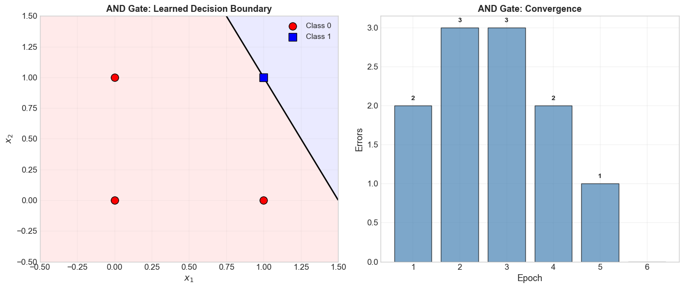
5.5 Learning the AND Gate#

============================================================
Training Perceptron on AND Gate
============================================================

Truth table:
  0 AND 0 = 0
  0 AND 1 = 0
  1 AND 0 = 0
  1 AND 1 = 1

  Epoch 1, sample 0: x=[0 0], y=0, y_hat=1, update=-1 -> w=[0. 0.], b=-1.0
  Epoch 1, sample 3: x=[1 1], y=1, y_hat=0, update=+1 -> w=[1. 1.], b=0.0
  Epoch 1: 2 errors
  Epoch 2, sample 0: x=[0 0], y=0, y_hat=1, update=-1 -> w=[1. 1.], b=-1.0
  Epoch 2, sample 1: x=[0 1], y=0, y_hat=1, update=-1 -> w=[1. 0.], b=-2.0
  Epoch 2, sample 3: x=[1 1], y=1, y_hat=0, update=+1 -> w=[2. 1.], b=-1.0
  Epoch 2: 3 errors
  Epoch 3, sample 1: x=[0 1], y=0, y_hat=1, update=-1 -> w=[2. 0.], b=-2.0
  Epoch 3, sample 2: x=[1 0], y=0, y_hat=1, update=-1 -> w=[1. 0.], b=-3.0
  Epoch 3, sample 3: x=[1 1], y=1, y_hat=0, update=+1 -> w=[2. 1.], b=-2.0
  Epoch 3: 3 errors
  Epoch 4, sample 2: x=[1 0], y=0, y_hat=1, update=-1 -> w=[1. 1.], b=-3.0
  Epoch 4, sample 3: x=[1 1], y=1, y_hat=0, update=+1 -> w=[2. 2.], b=-2.0
  Epoch 4: 2 errors
  Epoch 5, sample 1: x=[0 1], y=0, y_hat=1, update=-1 -> w=[2. 1.], b=-3.0
  Epoch 5: 1 errors
  Epoch 6: 0 errors

  Converged after 6 epochs!

Final model: Perceptron(w=[2. 1.], b=-3.0, converged=True)

Verification:
  [0 0] -> 0 (expected 0) [OK]
  [0 1] -> 0 (expected 0) [OK]
  [1 0] -> 0 (expected 0) [OK]
  [1 1] -> 1 (expected 1) [OK]

../_images/6518775ee2deff798e7e3faa0ae2b8487c5fc074717aba91f23e710722998270.png

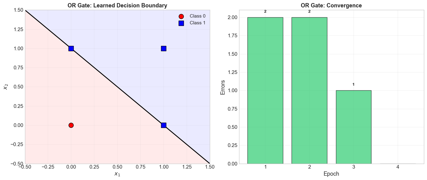
5.6 Learning the OR Gate#

============================================================
Training Perceptron on OR Gate
============================================================

Truth table:
  0 OR 0 = 0
  0 OR 1 = 1
  1 OR 0 = 1
  1 OR 1 = 1

  Epoch 1, sample 0: x=[0 0], y=0, y_hat=1, update=-1 -> w=[0. 0.], b=-1.0
  Epoch 1, sample 1: x=[0 1], y=1, y_hat=0, update=+1 -> w=[0. 1.], b=0.0
  Epoch 1: 2 errors
  Epoch 2, sample 0: x=[0 0], y=0, y_hat=1, update=-1 -> w=[0. 1.], b=-1.0
  Epoch 2, sample 2: x=[1 0], y=1, y_hat=0, update=+1 -> w=[1. 1.], b=0.0
  Epoch 2: 2 errors
  Epoch 3, sample 0: x=[0 0], y=0, y_hat=1, update=-1 -> w=[1. 1.], b=-1.0
  Epoch 3: 1 errors
  Epoch 4: 0 errors

  Converged after 4 epochs!

Final model: Perceptron(w=[1. 1.], b=-1.0, converged=True)

Verification:
  [0 0] -> 0 (expected 0) [OK]
  [0 1] -> 1 (expected 1) [OK]
  [1 0] -> 1 (expected 1) [OK]
  [1 1] -> 1 (expected 1) [OK]

../_images/e2688349ebafb98f4b85743398af5baba6b09f73203fee04a173f9c69d4668a1.png

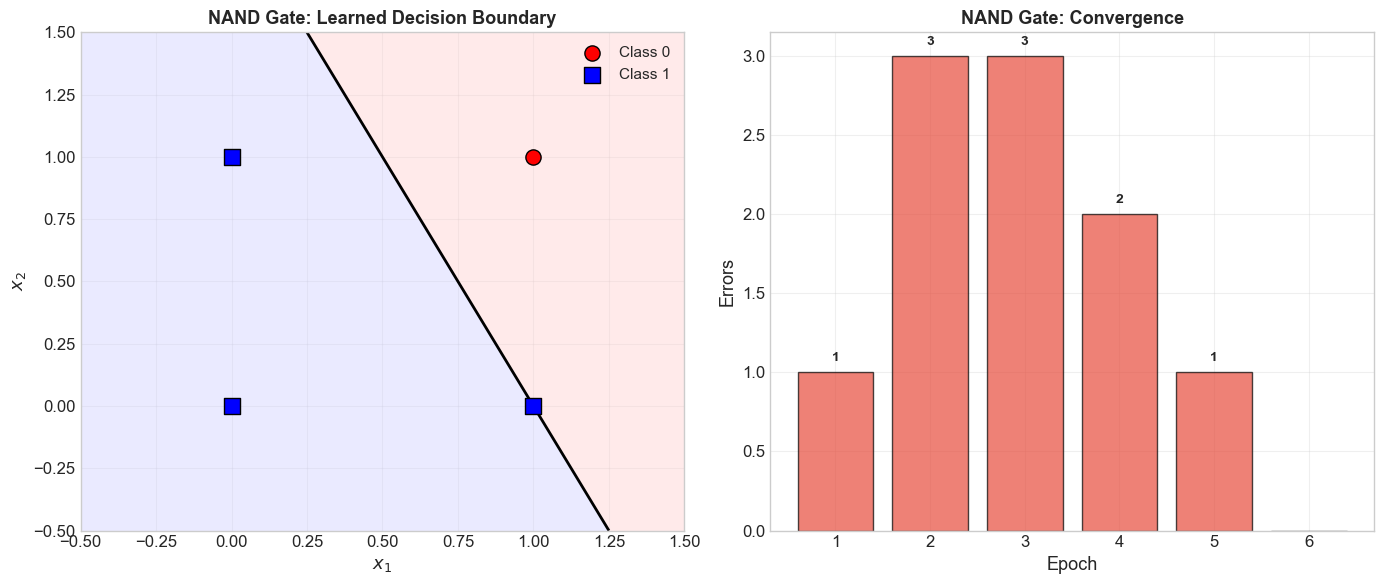
5.7 Learning the NAND Gate#

============================================================
Training Perceptron on NAND Gate
============================================================

Truth table:
  0 NAND 0 = 1
  0 NAND 1 = 1
  1 NAND 0 = 1
  1 NAND 1 = 0

  Epoch 1, sample 3: x=[1 1], y=0, y_hat=1, update=-1 -> w=[-1. -1.], b=-1.0
  Epoch 1: 1 errors
  Epoch 2, sample 0: x=[0 0], y=1, y_hat=0, update=+1 -> w=[-1. -1.], b=0.0
  Epoch 2, sample 1: x=[0 1], y=1, y_hat=0, update=+1 -> w=[-1.  0.], b=1.0
  Epoch 2, sample 3: x=[1 1], y=0, y_hat=1, update=-1 -> w=[-2. -1.], b=0.0
  Epoch 2: 3 errors
  Epoch 3, sample 1: x=[0 1], y=1, y_hat=0, update=+1 -> w=[-2.  0.], b=1.0
  Epoch 3, sample 2: x=[1 0], y=1, y_hat=0, update=+1 -> w=[-1.  0.], b=2.0
  Epoch 3, sample 3: x=[1 1], y=0, y_hat=1, update=-1 -> w=[-2. -1.], b=1.0
  Epoch 3: 3 errors
  Epoch 4, sample 2: x=[1 0], y=1, y_hat=0, update=+1 -> w=[-1. -1.], b=2.0
  Epoch 4, sample 3: x=[1 1], y=0, y_hat=1, update=-1 -> w=[-2. -2.], b=1.0
  Epoch 4: 2 errors
  Epoch 5, sample 1: x=[0 1], y=1, y_hat=0, update=+1 -> w=[-2. -1.], b=2.0
  Epoch 5: 1 errors
  Epoch 6: 0 errors

  Converged after 6 epochs!

Final model: Perceptron(w=[-2. -1.], b=2.0, converged=True)

Verification:
  [0 0] -> 1 (expected 1) [OK]
  [0 1] -> 1 (expected 1) [OK]
  [1 0] -> 1 (expected 1) [OK]
  [1 1] -> 0 (expected 0) [OK]

../_images/685fcee152fa91d46f18cd5577f1a677cb57cb64311906f67d39a5ce2c8496a2.png

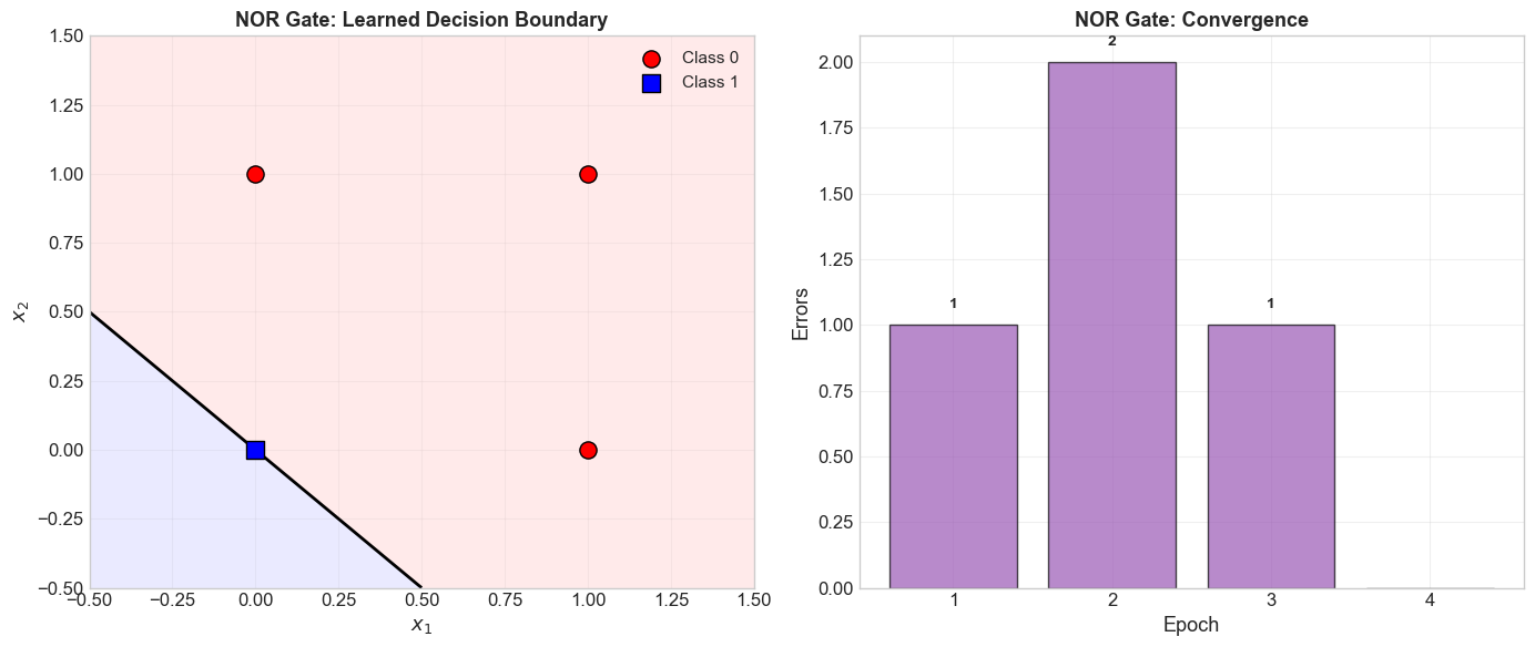
5.8 Learning the NOR Gate#

============================================================
Training Perceptron on NOR Gate
============================================================

Truth table:
  0 NOR 0 = 1
  0 NOR 1 = 0
  1 NOR 0 = 0
  1 NOR 1 = 0

  Epoch 1, sample 1: x=[0 1], y=0, y_hat=1, update=-1 -> w=[ 0. -1.], b=-1.0
  Epoch 1: 1 errors
  Epoch 2, sample 0: x=[0 0], y=1, y_hat=0, update=+1 -> w=[ 0. -1.], b=0.0
  Epoch 2, sample 2: x=[1 0], y=0, y_hat=1, update=-1 -> w=[-1. -1.], b=-1.0
  Epoch 2: 2 errors
  Epoch 3, sample 0: x=[0 0], y=1, y_hat=0, update=+1 -> w=[-1. -1.], b=0.0
  Epoch 3: 1 errors
  Epoch 4: 0 errors

  Converged after 4 epochs!

Final model: Perceptron(w=[-1. -1.], b=0.0, converged=True)

Verification:
  [0 0] -> 1 (expected 1) [OK]
  [0 1] -> 0 (expected 0) [OK]
  [1 0] -> 0 (expected 0) [OK]
  [1 1] -> 0 (expected 0) [OK]

../_images/1210573a2f12b43ae43307ba0e451a4351bfda63993d9e953f5f4cce58f9d6d0.png

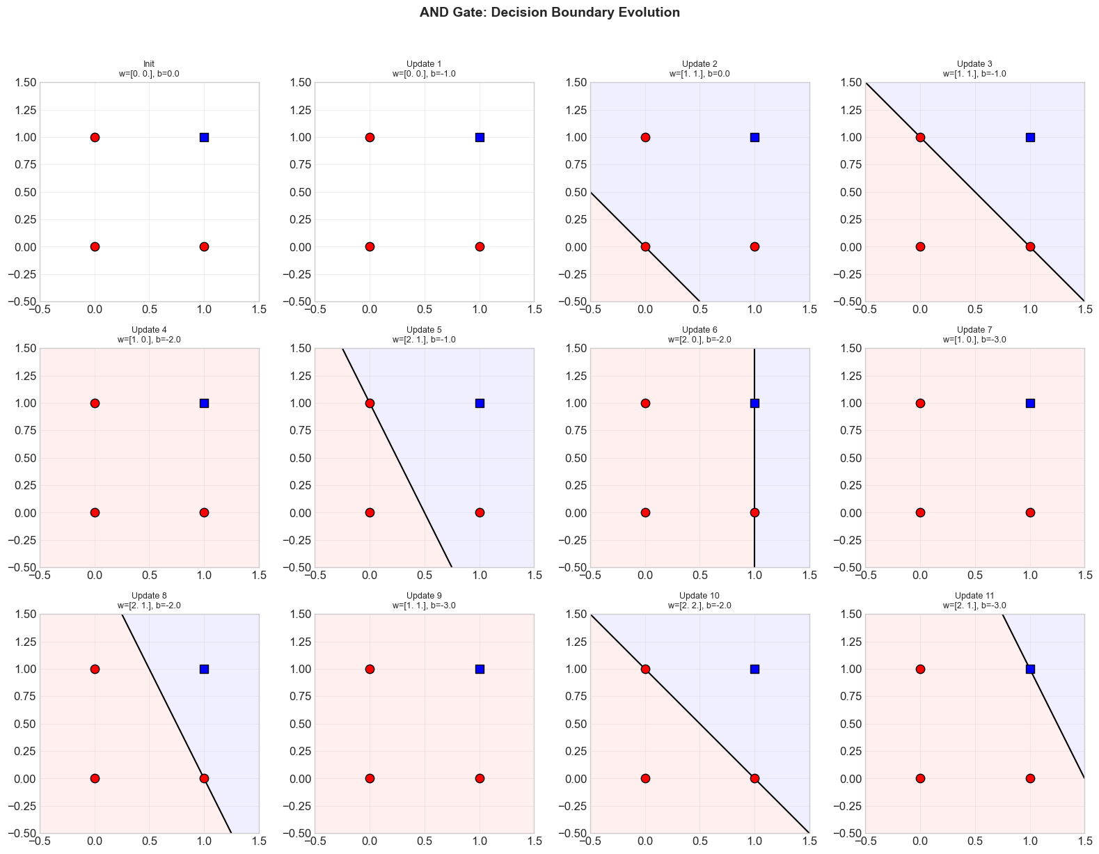
5.9 Decision Boundary Evolution#

One of the most instructive ways to understand the perceptron learning algorithm is to visualize how the decision boundary changes after each weight update. Below, we show the decision boundary at each snapshot in the weight history during training on the AND gate.

Show code cell source Hide code cell source

import numpy as np
import matplotlib.pyplot as plt

# Retrain AND gate and show boundary evolution
p_evo = Perceptron(n_features=2, learning_rate=1.0, max_epochs=20)
p_evo.fit(X_and, y_and)

n_snapshots = len(p_evo.weight_history)
n_cols = min(4, n_snapshots)
n_rows = (n_snapshots + n_cols - 1) // n_cols

fig, axes = plt.subplots(n_rows, n_cols, figsize=(4 * n_cols, 4 * n_rows))
if n_rows == 1 and n_cols == 1:
    axes = np.array([axes])
axes = np.atleast_2d(axes)

# Color map for evolution steps
cmap = plt.cm.viridis
colors = [cmap(i / max(n_snapshots - 1, 1)) for i in range(n_snapshots)]

for idx, (w_snap, b_snap) in enumerate(p_evo.weight_history):
    row, col = divmod(idx, n_cols)
    ax = axes[row, col]
    
    # Create mesh
    xx, yy = np.meshgrid(np.linspace(-0.5, 1.5, 200),
                         np.linspace(-0.5, 1.5, 200))
    
    w_norm = np.linalg.norm(w_snap)
    if w_norm > 0:
        Z = xx * w_snap[0] + yy * w_snap[1] + b_snap
        ax.contourf(xx, yy, Z, levels=[-1e10, 0, 1e10],
                    colors=['#FFCCCC', '#CCCCFF'], alpha=0.3)
        ax.contour(xx, yy, Z, levels=[0], colors='black', linewidths=1.5)
    
    ax.scatter(X_and[y_and == 0, 0], X_and[y_and == 0, 1],
               c='red', marker='o', s=80, edgecolors='black', zorder=5)
    ax.scatter(X_and[y_and == 1, 0], X_and[y_and == 1, 1],
               c='blue', marker='s', s=80, edgecolors='black', zorder=5)
    
    step_label = 'Init' if idx == 0 else f'Update {idx}'
    ax.set_title(f'{step_label}\nw={np.round(w_snap, 1)}, b={b_snap:.1f}',
                 fontsize=9)
    ax.set_xlim(-0.5, 1.5)
    ax.set_ylim(-0.5, 1.5)
    ax.set_aspect('equal')
    ax.grid(True, alpha=0.3)

# Hide empty axes
for idx in range(n_snapshots, n_rows * n_cols):
    row, col = divmod(idx, n_cols)
    axes[row, col].set_visible(False)

fig.suptitle('AND Gate: Decision Boundary Evolution',
             fontsize=14, fontweight='bold', y=1.02)
plt.tight_layout()
plt.show()

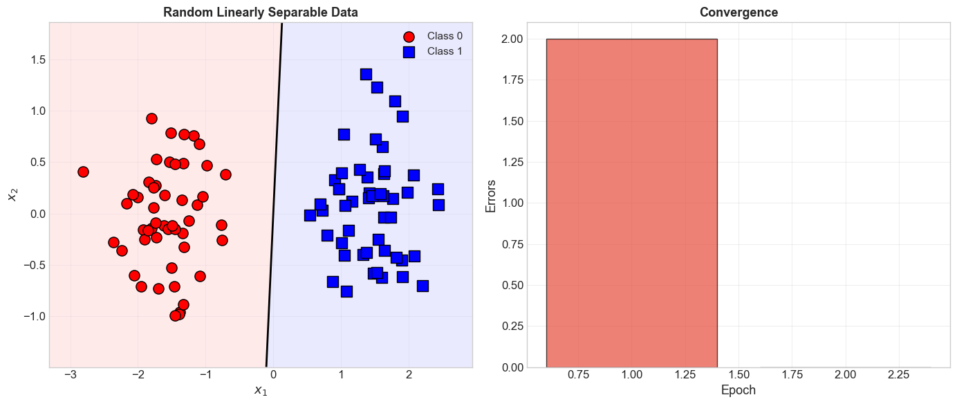
../_images/6c21017ccad76b373cf82a5d7acd8a81a23adb9337e92442e78d7db533ca25cf.png

5.10 Random Linearly Separable Data#

Converged: True
Epochs: 2
Final weights: [ 2.04395755 -0.14119051]
Final bias: 0.0

../_images/8f2cc23430b99d6a96dc5a47192a3e2f797870b9b54dbf3503b6774ee3892e28.png

Show code cell source Hide code cell source

import numpy as np
import matplotlib.pyplot as plt

# Experiment: How does cluster separation affect convergence speed?
separations = [1.0, 1.5, 2.0, 2.5, 3.0, 4.0, 5.0]
n_trials = 20
results = {}

for sep in separations:
    epoch_counts = []
    for trial in range(n_trials):
        X_trial, y_trial = generate_linearly_separable_data(
            n_per_class=30, separation=sep, seed=trial * 100 + int(sep * 10))
        p_trial = Perceptron(n_features=2, learning_rate=1.0, max_epochs=500)
        p_trial.fit(X_trial, y_trial)
        if p_trial.converged:
            epoch_counts.append(len(p_trial.errors_per_epoch))
    results[sep] = epoch_counts

# Plot results with enhanced styling
fig, ax = plt.subplots(figsize=(10, 6))

positions = list(range(len(separations)))
box_data = [results[s] for s in separations]

# Filter out empty lists for boxplot (matplotlib can't plot empty data)
non_empty_positions = [p for p, d in zip(positions, box_data) if len(d) > 0]
non_empty_data = [d for d in box_data if len(d) > 0]
non_empty_seps = [s for s, d in zip(separations, box_data) if len(d) > 0]

if non_empty_data:
    bp = ax.boxplot(non_empty_data, positions=non_empty_positions, widths=0.6, patch_artist=True)

    # Color gradient from red (hard) to green (easy)
    cmap = plt.cm.RdYlGn
    for i, patch in enumerate(bp['boxes']):
        color = cmap(non_empty_positions[i] / max(len(separations) - 1, 1))
        patch.set_facecolor(color)
        patch.set_alpha(0.7)

ax.set_xticks(positions)
ax.set_xticklabels([str(s) for s in separations])
ax.set_xlabel('Cluster Separation', fontsize=13)
ax.set_ylabel('Epochs to Convergence', fontsize=13)
ax.set_title('Effect of Cluster Separation on Convergence Speed',
             fontsize=14, fontweight='bold')
ax.grid(True, alpha=0.3, axis='y')

# Add annotation only if we have valid data for the endpoints
last_data = results[separations[-1]]
first_data = results[separations[0]]
if last_data and first_data:
    ax.annotate('Larger separation\n= faster convergence',
                xy=(len(separations)-1, np.mean(last_data)),
                xytext=(len(separations)-2.5, np.mean(first_data) + 3),
                fontsize=11, ha='center',
                arrowprops=dict(arrowstyle='->', color='green', lw=1.5),
                color='green', fontweight='bold')

plt.tight_layout()
plt.show()

print("\nSummary:")
print(f"{'Separation':>12} | {'Mean Epochs':>12} | {'Std':>8} | {'Converged':>10}")
print("-" * 52)
for sep in separations:
    data = results[sep]
    if data:
        print(f"{sep:>12.1f} | {np.mean(data):>12.1f} | {np.std(data):>8.1f} | {len(data):>10}/{n_trials}")
    else:
        print(f"{sep:>12.1f} | {'N/A':>12} | {'N/A':>8} | {0:>10}/{n_trials}")

../_images/fbd5fb5f800cbe55d8a913f3302c14bc37552d247ef2d98e86c753b1ea1bef3b.png

Summary:
  Separation |  Mean Epochs |      Std |  Converged
----------------------------------------------------
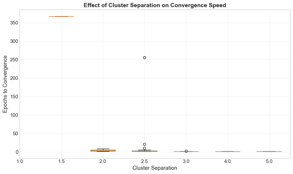
         1.0 |          N/A |      N/A |          0/20
         1.5 |        367.0 |      0.0 |          1/20
         2.0 |          4.4 |      2.4 |         12/20
         2.5 |         18.2 |     57.9 |         18/20
         3.0 |          2.0 |      0.2 |         20/20
         4.0 |          2.0 |      0.0 |         20/20
         5.0 |          2.0 |      0.0 |         20/20

Observation#

As cluster separation increases:

The margin \(\gamma\) between the classes grows.
By the Perceptron Convergence Theorem, the bound on mistakes is \(R^2/\gamma^2\), so larger \(\gamma\) means fewer mistakes.
The perceptron converges faster, often in just a few epochs.

5.11 Learning Rate Experiment#

eta=  0.1: converged=True, epochs=2, ||w||=0.19, b=0.00
eta=  0.5: converged=True, epochs=2, ||w||=0.93, b=0.00
eta=  1.0: converged=True, epochs=2, ||w||=1.86, b=0.00
eta=  5.0: converged=True, epochs=2, ||w||=9.28, b=0.00
eta= 10.0: converged=True, epochs=2, ||w||=18.56, b=0.00

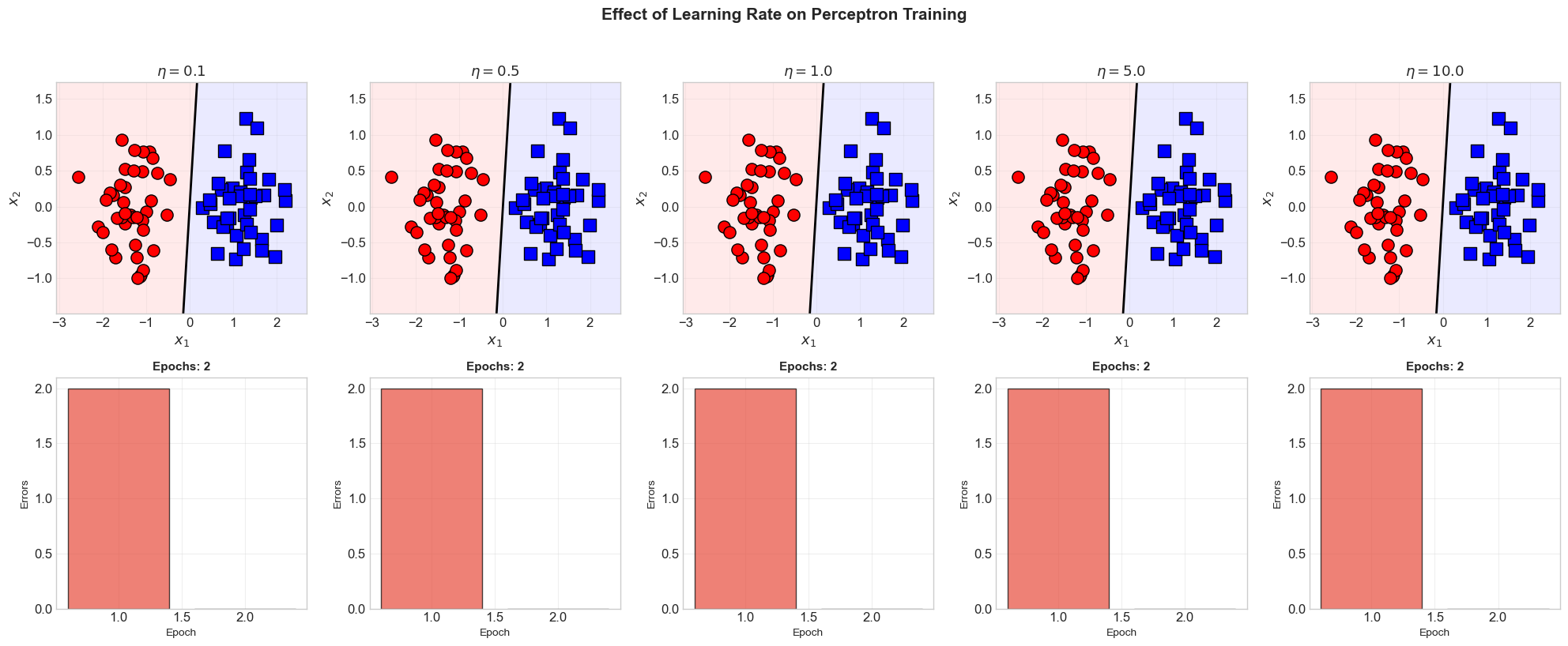
../_images/8fc403275f94011ddadb54a4be211e4fa38c43be1e652e4c0e2e1d9baff2c415.png

Key Insight: Learning Rate and the Step Function#

For the perceptron with a step activation function, the learning rate \(\eta\) does not affect whether the algorithm converges or the number of epochs required. Here is why:

The decision boundary depends only on the direction of \(\mathbf{w}\) and the ratio \(b/\|\mathbf{w}\|\).
Scaling all weights and bias by \(\eta\) does not change the decision boundary: \(\text{step}(\eta(\mathbf{w} \cdot \mathbf{x} + b)) = \text{step}(\mathbf{w} \cdot \mathbf{x} + b)\).
Different \(\eta\) values produce weight vectors that differ only in scale, not direction.

The number of update steps (mistakes) is the same regardless of \(\eta\). The norm \(\|\mathbf{w}\|\) scales linearly with \(\eta\), but the decision boundary is identical.

This is a special property of the step function. For differentiable activation functions (like the sigmoid), the learning rate plays a crucial role in convergence behavior.

5.12 Exercises#

Exercise 5.1: Custom Dataset#

Create your own 2D dataset (at least 10 points per class) that is linearly separable. Train the perceptron on it and visualize the result. Try different initializations and orderings of the training data. Does the final boundary change?

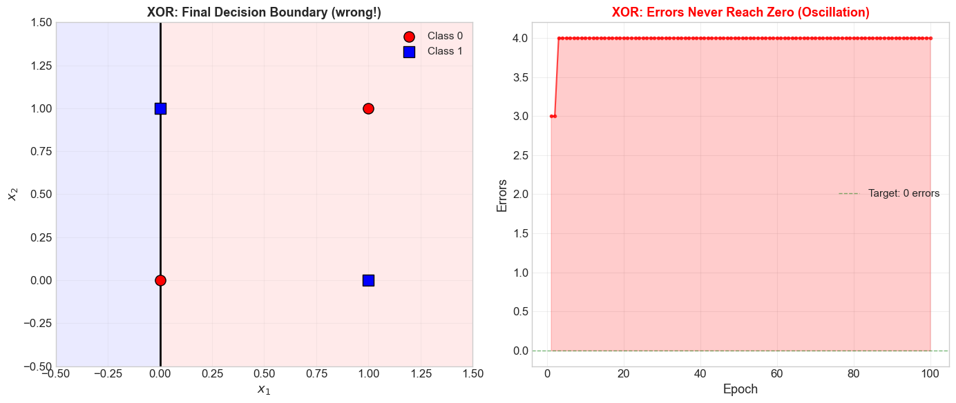
Exercise 5.2: The XOR Disaster#

Train the perceptron on the XOR truth table. Run for 100 epochs.

Does it converge? Why or why not?
Plot the errors per epoch. What pattern do you observe?
Plot the decision boundary at the final epoch. Is any configuration of \(\mathbf{w}\) and \(b\) a valid solution?

Exercise 5.3: The {-1, +1} Variant#

Implement the perceptron learning algorithm using labels \(y \in \{-1, +1\}\) and the sign function. The update rule becomes:

\[\mathbf{w}_{t+1} = \mathbf{w}_t + \eta \cdot y_i \cdot \mathbf{x}_i \quad \text{(on misclassification)}\]

Train on the AND gate (relabeling 0 as -1) and verify it gives the same decision boundary.

============================================================
Attempting to Learn XOR
============================================================

Converged: False
Epochs run: 100
Final weights: [-1.  0.]
Final bias: 0.0

Verification:
  [0 0] -> 1 (expected 0) [WRONG]
  [0 1] -> 1 (expected 1) [OK]
  [1 0] -> 0 (expected 1) [WRONG]
  [1 1] -> 0 (expected 0) [OK]

../_images/df31d08a27808a271bc7dd0fda8d4f9fcd5d2120b2687251be0203137cee9106.png