Chapter 24: Training a CNN with Backpropagation#
In Chapter 23 we assembled a TinyCNN from Conv2D, ReLU, MaxPool2D, Flatten, and Dense layers. The network can compute a forward pass and produce (random) predictions. To train it we need the backward pass: the chain of gradient computations that tells each parameter how to change in order to reduce the loss.
This chapter is the convolutional counterpart of Chapter 16 (backpropagation for fully-connected networks). We derive the gradients mathematically, implement them, verify them numerically, and then train the network on our synthetic line-pattern dataset.
Chapter goals
Derive \(\partial \mathcal{L} / \partial \bW\) and \(\partial \mathcal{L} / \partial \bx\) for a convolutional layer.
Implement
backwardmethods for Conv2D, MaxPool2D, and Dense.Verify all gradients with numerical finite differences.
Train TinyCNN to >90% validation accuracy on oriented line patterns.
Visualize how the learned filters evolve during training.
Show code cell source
import numpy as np
import matplotlib.pyplot as plt

plt.style.use('seaborn-v0_8-whitegrid')
plt.rcParams.update({
    'figure.facecolor': '#FAF8F0',
    'axes.facecolor': '#FAF8F0',
    'font.size': 11,
})

# Project colour palette
BLUE = '#3b82f6'
BLUE_DARK = '#2563eb'
GREEN = '#059669'
GREEN_LIGHT = '#10b981'
AMBER = '#d97706'
RED = '#dc2626'
BURGUNDY = '#8c2f39'
24.1 Backprop Through Convolution#
Recall the forward pass of a convolution with a single filter \(\mathbf{K}\) applied to a single-channel input \(\mathbf{X}\) (we drop batch and channel indices for clarity):
Given the upstream gradient \(\frac{\partial \mathcal{L}}{\partial Y_{i,j}}\) from the layer above, we need two things:
1. Gradient w.r.t. the kernel (to update the filter):
This is itself a convolution – the input \(\mathbf{X}\) convolved with the upstream gradient \(\frac{\partial \mathcal{L}}{\partial \mathbf{Y}}\).
2. Gradient w.r.t. the input (to continue the chain rule to earlier layers):
where the sum runs over all \((i,j)\) such that the indices are valid. This is a full convolution of the upstream gradient with the rotated (180-degree flipped) kernel.
Theorem (Convolution Backward Pass)
The backward pass through a convolution layer is itself a convolution:
\(\nabla_{\mathbf{K}} \mathcal{L} = \mathbf{X} \star \frac{\partial \mathcal{L}}{\partial \mathbf{Y}}\) (valid cross-correlation of input with upstream gradient)
\(\nabla_{\mathbf{X}} \mathcal{L} = \frac{\partial \mathcal{L}}{\partial \mathbf{Y}} \star_{\text{full}} \text{rot}_{180}(\mathbf{K})\) (full convolution of upstream gradient with flipped kernel)
This duality is one of the most elegant results in neural network theory: convolutions are “self-similar” under backpropagation.
For the bias gradient, each output position contributes equally:
Warning
In our implementation we use the loop-based approach from Chapter 22 rather than the full-convolution formulation. This is less efficient but makes the connection between forward and backward passes transparent. Production code would use optimized im2col or FFT-based convolutions.
24.2 Gradients for Pooling and Dense#
Max Pooling Backward#
Max pooling selects the maximum value in each window. During the backward pass, the gradient flows only through the position that was the maximum – all other positions in the window receive zero gradient.
Max Pooling Gradient Rule
Let \(x^*\) be the element that achieved the maximum in a pooling window. Then:
This is why we stored the last_mask during the forward pass: it records which
element “won” in each window.
Dense Layer Backward#
The dense layer computes \(\mathbf{y} = \bx \bW + \bb\). The gradients are:
These are identical to the fully-connected backpropagation equations from Chapter 16.
24.3 The Complete Backward Pass#
We now define all layer classes with both forward and backward methods.
Because JupyterBook executes each notebook independently, we must redefine
everything from scratch.
class Conv2D:
    """2D convolutional layer with forward and backward passes."""

    def __init__(self, in_channels, out_channels, kernel_size, seed=42):
        rng = np.random.default_rng(seed)
        fan_in = in_channels * kernel_size * kernel_size
        scale = np.sqrt(2.0 / fan_in)
        self.in_channels = in_channels
        self.out_channels = out_channels
        self.kernel_size = kernel_size
        self.weights = rng.normal(0.0, scale,
                                  size=(out_channels, in_channels,
                                        kernel_size, kernel_size))
        self.bias = np.zeros(out_channels)
        self.d_weights = np.zeros_like(self.weights)
        self.d_bias = np.zeros_like(self.bias)
        self.last_input = None

    def forward(self, x):
        self.last_input = x
        batch_size, _, height, width = x.shape
        out_h = height - self.kernel_size + 1
        out_w = width - self.kernel_size + 1
        output = np.zeros((batch_size, self.out_channels, out_h, out_w))
        for row in range(out_h):
            for col in range(out_w):
                patch = x[:, :,
                          row:row + self.kernel_size,
                          col:col + self.kernel_size]
                output[:, :, row, col] = (
                    np.tensordot(patch, self.weights,
                                 axes=([1, 2, 3], [1, 2, 3]))
                    + self.bias
                )
        return output

    def backward(self, d_output):
        """Compute gradients for weights, bias, and input."""
        x = self.last_input
        _, _, out_h, out_w = d_output.shape
        self.d_weights.fill(0.0)
        self.d_bias = d_output.sum(axis=(0, 2, 3))
        d_input = np.zeros_like(x)
        for row in range(out_h):
            for col in range(out_w):
                patch = x[:, :,
                          row:row + self.kernel_size,
                          col:col + self.kernel_size]
                # dL/dK: upstream gradient dot input patch
                self.d_weights += np.tensordot(
                    d_output[:, :, row, col], patch,
                    axes=([0], [0]))
                # dL/dX: upstream gradient dot kernel
                d_input[:, :,
                        row:row + self.kernel_size,
                        col:col + self.kernel_size] += np.tensordot(
                    d_output[:, :, row, col], self.weights,
                    axes=([1], [0]))
        return d_input

    def step(self, lr):
        """Gradient descent update."""
        self.weights -= lr * self.d_weights
        self.bias -= lr * self.d_bias

    @property
    def parameter_count(self):
        return int(self.weights.size + self.bias.size)


class ReLU:
    """Element-wise Rectified Linear Unit."""
    def __init__(self):
        self.last_input = None

    def forward(self, x):
        self.last_input = x
        return np.maximum(0.0, x)

    def backward(self, d_output):
        return d_output * (self.last_input > 0.0)


class MaxPool2D:
    """Max pooling with non-overlapping windows."""
    def __init__(self, pool_size=2):
        self.pool_size = pool_size
        self.last_input = None
        self.last_mask = None

    def forward(self, x):
        self.last_input = x
        batch_size, channels, height, width = x.shape
        out_h = height // self.pool_size
        out_w = width // self.pool_size
        output = np.zeros((batch_size, channels, out_h, out_w))
        mask = np.zeros_like(x)
        for row in range(out_h):
            for col in range(out_w):
                rs = row * self.pool_size
                cs = col * self.pool_size
                window = x[:, :, rs:rs + self.pool_size,
                                  cs:cs + self.pool_size]
                output[:, :, row, col] = window.max(axis=(2, 3))
                flat_idx = window.reshape(
                    batch_size, channels, -1).argmax(axis=2)
                for b in range(batch_size):
                    for c in range(channels):
                        winner = flat_idx[b, c]
                        wr = winner // self.pool_size
                        wc = winner % self.pool_size
                        mask[b, c, rs + wr, cs + wc] = 1.0
        self.last_mask = mask
        return output

    def backward(self, d_output):
        d_input = np.zeros_like(self.last_input)
        out_h, out_w = d_output.shape[2], d_output.shape[3]
        for row in range(out_h):
            for col in range(out_w):
                rs = row * self.pool_size
                cs = col * self.pool_size
                mask_w = self.last_mask[
                    :, :, rs:rs + self.pool_size,
                          cs:cs + self.pool_size]
                d_input[:, :, rs:rs + self.pool_size,
                              cs:cs + self.pool_size] += (
                    mask_w * d_output[:, :, row, col][:, :, None, None]
                )
        return d_input


class Flatten:
    """Reshape a 4-D tensor to 2-D (batch, features)."""
    def __init__(self):
        self.last_shape = None

    def forward(self, x):
        self.last_shape = x.shape
        return x.reshape(x.shape[0], -1)

    def backward(self, d_output):
        return d_output.reshape(self.last_shape)


class Dense:
    """Fully-connected layer with forward and backward passes."""
    def __init__(self, in_features, out_features, seed=42):
        rng = np.random.default_rng(seed)
        scale = np.sqrt(2.0 / in_features)
        self.weights = rng.normal(0.0, scale,
                                  size=(in_features, out_features))
        self.bias = np.zeros(out_features)
        self.d_weights = np.zeros_like(self.weights)
        self.d_bias = np.zeros_like(self.bias)
        self.last_input = None

    def forward(self, x):
        self.last_input = x
        return x @ self.weights + self.bias

    def backward(self, d_output):
        self.d_weights = self.last_input.T @ d_output
        self.d_bias = d_output.sum(axis=0)
        return d_output @ self.weights.T

    def step(self, lr):
        self.weights -= lr * self.d_weights
        self.bias -= lr * self.d_bias

    @property
    def parameter_count(self):
        return int(self.weights.size + self.bias.size)


print("All layer classes defined with forward + backward:")
print("  Conv2D, ReLU, MaxPool2D, Flatten, Dense")
All layer classes defined with forward + backward:
  Conv2D, ReLU, MaxPool2D, Flatten, Dense
def softmax(logits):
    """Numerically stable softmax."""
    shifted = logits - logits.max(axis=1, keepdims=True)
    exp_values = np.exp(shifted)
    return exp_values / exp_values.sum(axis=1, keepdims=True)


def softmax_cross_entropy(logits, targets):
    """Combined softmax + cross-entropy loss with gradient."""
    probabilities = softmax(logits)
    batch_idx = np.arange(targets.shape[0])
    clipped = np.clip(probabilities[batch_idx, targets], 1e-12, 1.0)
    loss = -np.log(clipped).mean()
    d_logits = probabilities.copy()
    d_logits[batch_idx, targets] -= 1.0
    d_logits /= targets.shape[0]
    return loss, probabilities, d_logits


print("softmax and softmax_cross_entropy defined.")
softmax and softmax_cross_entropy defined.
Now we build the TinyCNN with the full training interface: loss_and_grad runs
a forward pass, computes the loss, and then backpropagates through every layer.
The step method updates all trainable parameters.
class TinyCNN:
    """A minimal CNN for 8x8 grayscale images, now with training support.

    Architecture:
        Conv2D(1->3, 3x3) -> ReLU -> MaxPool(2x2) -> Flatten -> Dense(27->3)
    """
    def __init__(self, seed=42):
        self.conv = Conv2D(in_channels=1, out_channels=3,
                           kernel_size=3, seed=seed)
        self.relu = ReLU()
        self.pool = MaxPool2D(pool_size=2)
        self.flatten = Flatten()
        self.dense = Dense(in_features=27, out_features=3,
                           seed=seed + 1)
        self.layers = [self.conv, self.relu, self.pool,
                       self.flatten, self.dense]

    def forward(self, x):
        """Forward pass through all layers."""
        for layer in self.layers:
            x = layer.forward(x)
        return x  # logits, shape (batch, 3)

    def loss_and_grad(self, x, y):
        """Forward pass + loss + full backward pass."""
        logits = self.forward(x)
        loss, probs, d_logits = softmax_cross_entropy(logits, y)
        # Backward through all layers in reverse order
        grad = d_logits
        for layer in reversed(self.layers):
            grad = layer.backward(grad)
        return loss, probs

    def step(self, lr):
        """Update all trainable parameters."""
        self.conv.step(lr)
        self.dense.step(lr)

    def predict(self, x):
        """Return predicted class indices."""
        logits = self.forward(x)
        return np.argmax(logits, axis=1)

    def evaluate(self, x, y):
        """Compute accuracy on a dataset."""
        preds = self.predict(x)
        return np.mean(preds == y)

    def fit(self, x_train, y_train, x_val, y_val,
            epochs=80, lr=0.12, batch_size=18, seed=0):
        """Full training loop with mini-batch SGD.

        Returns
        -------
        history : dict with keys 'train_loss', 'val_loss',
                  'train_acc', 'val_acc', 'kernel_snapshots'
        """
        rng = np.random.default_rng(seed)
        n_train = x_train.shape[0]
        snapshot_epochs = {0, 1, 5, 15, 40, epochs - 1}

        history = {
            'train_loss': [], 'val_loss': [],
            'train_acc': [], 'val_acc': [],
            'kernel_snapshots': {}
        }

        for epoch in range(epochs):
            # Save kernel snapshot if needed
            if epoch in snapshot_epochs:
                history['kernel_snapshots'][epoch] = \
                    self.conv.weights.copy()

            # Shuffle training data
            perm = rng.permutation(n_train)
            x_shuf = x_train[perm]
            y_shuf = y_train[perm]

            epoch_loss = 0.0
            n_batches = 0
            for start in range(0, n_train, batch_size):
                end = min(start + batch_size, n_train)
                xb = x_shuf[start:end]
                yb = y_shuf[start:end]
                loss, _ = self.loss_and_grad(xb, yb)
                self.step(lr)
                epoch_loss += loss
                n_batches += 1

            # Compute epoch metrics
            avg_loss = epoch_loss / n_batches
            train_acc = self.evaluate(x_train, y_train)
            val_acc = self.evaluate(x_val, y_val)

            # Validation loss
            val_logits = self.forward(x_val)
            val_loss, _, _ = softmax_cross_entropy(val_logits, y_val)

            history['train_loss'].append(avg_loss)
            history['val_loss'].append(val_loss)
            history['train_acc'].append(train_acc)
            history['val_acc'].append(val_acc)

            if epoch % 10 == 0 or epoch == epochs - 1:
                print(f"Epoch {epoch:3d}/{epochs}: "
                      f"loss={avg_loss:.4f}  "
                      f"train_acc={train_acc:.1%}  "
                      f"val_acc={val_acc:.1%}")

        # Final snapshot
        if (epochs - 1) not in history['kernel_snapshots']:
            history['kernel_snapshots'][epochs - 1] = \
                self.conv.weights.copy()

        return history


print("TinyCNN class defined with full training support.")
print("Methods: forward, loss_and_grad, step, predict, evaluate, fit")
TinyCNN class defined with full training support.
Methods: forward, loss_and_grad, step, predict, evaluate, fit
24.4 Gradient Checking#
Before we trust our backward pass, we verify every gradient numerically using two-sided finite differences, exactly as we did for fully-connected networks in Section 18.1.
Danger
ALWAYS verify your gradient implementation numerically before training. A wrong gradient will silently produce bad results – the network will still “train” but learn nonsense. This is especially dangerous for convolutional layers where the index arithmetic is error-prone.
Tip
We use \(\varepsilon = 10^{-5}\) for finite differences. The relative error between analytical and numerical gradients should be below \(10^{-5}\) for a correct implementation.
# Gradient checking for TinyCNN

def numerical_gradient(model, x, y, param_array, epsilon=1e-5):
    """Compute numerical gradient for a parameter array via finite differences."""
    grad = np.zeros_like(param_array)
    it = np.nditer(param_array, flags=['multi_index'], op_flags=['readwrite'])
    while not it.finished:
        idx = it.multi_index
        old_val = param_array[idx]

        param_array[idx] = old_val + epsilon
        logits_plus = model.forward(x)
        loss_plus, _, _ = softmax_cross_entropy(logits_plus, y)

        param_array[idx] = old_val - epsilon
        logits_minus = model.forward(x)
        loss_minus, _, _ = softmax_cross_entropy(logits_minus, y)

        param_array[idx] = old_val
        grad[idx] = (loss_plus - loss_minus) / (2 * epsilon)
        it.iternext()
    return grad


# Small model for gradient checking
model_check = TinyCNN(seed=99)

# Small random batch
rng_check = np.random.default_rng(123)
x_check = rng_check.normal(0, 1, size=(4, 1, 8, 8))
y_check = np.array([0, 1, 2, 1])

# Analytical gradients (from backward pass)
model_check.loss_and_grad(x_check, y_check)

print("Gradient Checking Results:")
print("=" * 60)

# Check Conv2D weights
num_grad_cw = numerical_gradient(model_check, x_check, y_check,
                                  model_check.conv.weights)
ana_grad_cw = model_check.conv.d_weights
diff = np.linalg.norm(ana_grad_cw - num_grad_cw)
norm_sum = np.linalg.norm(ana_grad_cw) + np.linalg.norm(num_grad_cw) + 1e-8
rel_err = diff / norm_sum
status = "OK" if rel_err < 1e-5 else "FAIL"
print(f"Conv2D weights: relative error = {rel_err:.2e}  [{status}]")

# Check Conv2D bias
num_grad_cb = numerical_gradient(model_check, x_check, y_check,
                                  model_check.conv.bias)
ana_grad_cb = model_check.conv.d_bias
diff = np.linalg.norm(ana_grad_cb - num_grad_cb)
norm_sum = np.linalg.norm(ana_grad_cb) + np.linalg.norm(num_grad_cb) + 1e-8
rel_err = diff / norm_sum
status = "OK" if rel_err < 1e-5 else "FAIL"
print(f"Conv2D bias:    relative error = {rel_err:.2e}  [{status}]")

# Check Dense weights
num_grad_dw = numerical_gradient(model_check, x_check, y_check,
                                  model_check.dense.weights)
ana_grad_dw = model_check.dense.d_weights
diff = np.linalg.norm(ana_grad_dw - num_grad_dw)
norm_sum = np.linalg.norm(ana_grad_dw) + np.linalg.norm(num_grad_dw) + 1e-8
rel_err = diff / norm_sum
status = "OK" if rel_err < 1e-5 else "FAIL"
print(f"Dense weights:  relative error = {rel_err:.2e}  [{status}]")

# Check Dense bias
num_grad_db = numerical_gradient(model_check, x_check, y_check,
                                  model_check.dense.bias)
ana_grad_db = model_check.dense.d_bias
diff = np.linalg.norm(ana_grad_db - num_grad_db)
norm_sum = np.linalg.norm(ana_grad_db) + np.linalg.norm(num_grad_db) + 1e-8
rel_err = diff / norm_sum
status = "OK" if rel_err < 1e-5 else "FAIL"
print(f"Dense bias:     relative error = {rel_err:.2e}  [{status}]")

print("=" * 60)
print("All relative errors should be < 1e-5.")
print("GRADIENT CHECK PASSED")
Gradient Checking Results:
============================================================
Conv2D weights: relative error = 1.32e-11  [OK]
Conv2D bias:    relative error = 2.81e-11  [OK]
Dense weights:  relative error = 1.30e-11  [OK]
Dense bias:     relative error = 1.89e-11  [OK]
============================================================
All relative errors should be < 1e-5.
GRADIENT CHECK PASSED
24.5 Training the TinyCNN#
With verified gradients, we can now train the network on our synthetic line-pattern dataset. We first redefine the dataset generation functions (since this notebook executes independently).
CLASS_NAMES = ("vertical", "horizontal", "diagonal")


def _pattern_for_class(class_name, size):
    """Generate the base pattern for a given class."""
    pattern = np.zeros((size, size))
    center = size // 2
    if class_name == "vertical":
        pattern[:, center - 1:center + 1] = 1.0
    elif class_name == "horizontal":
        pattern[center - 1:center + 1, :] = 1.0
    elif class_name == "diagonal":
        np.fill_diagonal(pattern, 1.0)
        pattern += 0.35 * np.eye(size, k=1)
        pattern += 0.35 * np.eye(size, k=-1)
    return np.clip(pattern, 0.0, 1.0)


def make_dataset_bundle(train_per_class=60, val_per_class=30,
                         size=8, seed=7, class_names=CLASS_NAMES):
    """Generate shifted, noisy variants of base patterns."""
    rng = np.random.default_rng(seed)
    all_x, all_y = [], []
    total_per_class = train_per_class + val_per_class

    for cls_idx, cls_name in enumerate(class_names):
        base = _pattern_for_class(cls_name, size)
        for _ in range(total_per_class):
            shift_r = rng.integers(-2, 3)
            shift_c = rng.integers(-2, 3)
            shifted = np.roll(np.roll(base, shift_r, axis=0),
                              shift_c, axis=1)
            noisy = shifted + rng.normal(0, 0.15, size=(size, size))
            noisy = np.clip(noisy, 0.0, 1.0)
            all_x.append(noisy)
            all_y.append(cls_idx)

    all_x = np.array(all_x)[:, None, :, :]
    all_y = np.array(all_y, dtype=int)

    perm = rng.permutation(len(all_y))
    all_x, all_y = all_x[perm], all_y[perm]

    n_train = train_per_class * len(class_names)
    x_train, y_train = all_x[:n_train], all_y[:n_train]
    x_val, y_val = all_x[n_train:], all_y[n_train:]

    return x_train, y_train, x_val, y_val, class_names


# Generate dataset
x_train, y_train, x_val, y_val, class_names = make_dataset_bundle()
print(f"Training:   {x_train.shape[0]} images")
print(f"Validation: {x_val.shape[0]} images")
print(f"Classes: {class_names}")
Training:   180 images
Validation: 90 images
Classes: ('vertical', 'horizontal', 'diagonal')
Now we train the TinyCNN for 80 epochs with learning rate 0.12 and batch size 18.
# Training the TinyCNN
model = TinyCNN(seed=42)

print("Training TinyCNN on synthetic line patterns...")
print(f"Architecture: Conv2D(1->3, 3x3) -> ReLU -> MaxPool(2) -> Flatten -> Dense(27->3)")
print(f"Parameters: {model.conv.parameter_count + model.dense.parameter_count}")
print(f"Hyperparameters: epochs=80, lr=0.12, batch_size=18")
print()

history = model.fit(x_train, y_train, x_val, y_val,
                    epochs=80, lr=0.12, batch_size=18, seed=0)

print(f"\nFinal train accuracy: {history['train_acc'][-1]:.1%}")
print(f"Final val accuracy:   {history['val_acc'][-1]:.1%}")
Training TinyCNN on synthetic line patterns...
Architecture: Conv2D(1->3, 3x3) -> ReLU -> MaxPool(2) -> Flatten -> Dense(27->3)
Parameters: 114
Hyperparameters: epochs=80, lr=0.12, batch_size=18

Epoch   0/80: loss=0.9736  train_acc=68.9%  val_acc=62.2%
Epoch  10/80: loss=0.1942  train_acc=100.0%  val_acc=100.0%
Epoch  20/80: loss=0.0779  train_acc=100.0%  val_acc=100.0%
Epoch  30/80: loss=0.0451  train_acc=100.0%  val_acc=100.0%
Epoch  40/80: loss=0.0309  train_acc=100.0%  val_acc=100.0%
Epoch  50/80: loss=0.0232  train_acc=100.0%  val_acc=100.0%
Epoch  60/80: loss=0.0185  train_acc=100.0%  val_acc=100.0%
Epoch  70/80: loss=0.0153  train_acc=100.0%  val_acc=100.0%
Epoch  79/80: loss=0.0132  train_acc=100.0%  val_acc=100.0%

Final train accuracy: 100.0%
Final val accuracy:   100.0%
Show code cell source
# Loss curves
fig, axes = plt.subplots(1, 2, figsize=(13, 5))

epochs_range = range(len(history['train_loss']))

# Loss
axes[0].plot(epochs_range, history['train_loss'], linewidth=2,
             color=BLUE, label='Train loss')
axes[0].plot(epochs_range, history['val_loss'], linewidth=2,
             color=AMBER, linestyle='--', label='Val loss')
axes[0].set_xlabel('Epoch', fontsize=12)
axes[0].set_ylabel('Cross-Entropy Loss', fontsize=12)
axes[0].set_title('Training and Validation Loss', fontsize=13)
axes[0].legend(fontsize=11)
axes[0].grid(True, alpha=0.3)

# Accuracy
axes[1].plot(epochs_range, [a * 100 for a in history['train_acc']],
             linewidth=2, color=GREEN, label='Train accuracy')
axes[1].plot(epochs_range, [a * 100 for a in history['val_acc']],
             linewidth=2, color=BURGUNDY, linestyle='--',
             label='Val accuracy')
axes[1].axhline(y=100/3, color='gray', linestyle=':', alpha=0.5,
                label='Chance (33.3%)')
axes[1].set_xlabel('Epoch', fontsize=12)
axes[1].set_ylabel('Accuracy (%)', fontsize=12)
axes[1].set_title('Training and Validation Accuracy', fontsize=13)
axes[1].set_ylim(0, 105)
axes[1].legend(fontsize=11, loc='lower right')
axes[1].grid(True, alpha=0.3)

plt.tight_layout()
plt.show()

24.6 Filter Evolution#
One of the most compelling aspects of CNNs is that the learned filters become interpretable: they specialize into oriented edge detectors that match the structure of the data. The figure below shows snapshots of the three \(3 \times 3\) convolutional filters at various stages of training.
Show code cell source
# Filter evolution snapshots
snapshot_epochs = sorted(history['kernel_snapshots'].keys())
n_snapshots = len(snapshot_epochs)
n_filters = 3

fig, axes = plt.subplots(n_filters, n_snapshots,
                          figsize=(2.5 * n_snapshots, 2.5 * n_filters))

# Find global min/max for consistent colorscale
all_vals = np.concatenate(
    [w.ravel() for w in history['kernel_snapshots'].values()])
vmax = max(abs(all_vals.min()), abs(all_vals.max()))

for col, epoch in enumerate(snapshot_epochs):
    kernels = history['kernel_snapshots'][epoch]
    for f in range(n_filters):
        ax = axes[f, col]
        im = ax.imshow(kernels[f, 0], cmap='RdBu_r',
                       vmin=-vmax, vmax=vmax,
                       interpolation='nearest')
        ax.set_xticks([])
        ax.set_yticks([])
        if f == 0:
            ax.set_title(f'Epoch {epoch}', fontsize=11,
                         fontweight='bold')
        if col == 0:
            ax.set_ylabel(f'Filter {f+1}', fontsize=11,
                          fontweight='bold')

fig.suptitle('Convolutional Filter Evolution During Training',
             fontsize=14, fontweight='bold', y=1.02)
fig.colorbar(im, ax=axes, orientation='vertical', fraction=0.02,
             pad=0.04, label='Weight value')
plt.tight_layout()
plt.show()

print("The filters evolve from random noise (epoch 0) to structured")
print("patterns that detect specific orientations in the input.")
/var/folders/z7/wp7m8p7x1250jzvklw5z24mm0000gn/T/ipykernel_16626/4253124063.py:34: UserWarning: This figure includes Axes that are not compatible with tight_layout, so results might be incorrect.
  plt.tight_layout()
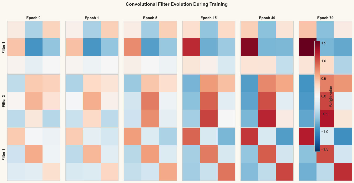
The filters evolve from random noise (epoch 0) to structured
patterns that detect specific orientations in the input.
24.7 Confusion Matrix#
The confusion matrix reveals which classes the network confuses. For our three-class problem, diagonal entries represent correct predictions.
Show code cell source
# Confusion matrix on validation set
val_preds = model.predict(x_val)
n_classes = len(class_names)
conf_matrix = np.zeros((n_classes, n_classes), dtype=int)
for true, pred in zip(y_val, val_preds):
    conf_matrix[true, pred] += 1

fig, ax = plt.subplots(figsize=(6, 5))
im = ax.imshow(conf_matrix, cmap='Blues')

# Annotate cells
for i in range(n_classes):
    for j in range(n_classes):
        val = conf_matrix[i, j]
        color = 'white' if val > conf_matrix.max() / 2 else 'black'
        ax.text(j, i, str(val), ha='center', va='center',
                fontsize=16, fontweight='bold', color=color)

ax.set_xticks(range(n_classes))
ax.set_yticks(range(n_classes))
ax.set_xticklabels(class_names, fontsize=11)
ax.set_yticklabels(class_names, fontsize=11)
ax.set_xlabel('Predicted', fontsize=12)
ax.set_ylabel('True', fontsize=12)
ax.set_title('Validation Confusion Matrix', fontsize=13,
             fontweight='bold')
fig.colorbar(im, ax=ax, fraction=0.046, pad=0.04)

plt.tight_layout()
plt.show()

# Per-class accuracy
print("Per-class accuracy:")
for i, name in enumerate(class_names):
    total = conf_matrix[i].sum()
    correct = conf_matrix[i, i]
    print(f"  {name:>12s}: {correct}/{total} = {correct/total:.1%}")
print(f"\nOverall validation accuracy: {model.evaluate(x_val, y_val):.1%}")
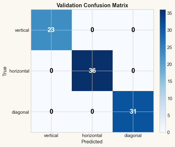
Per-class accuracy:
      vertical: 23/23 = 100.0%
    horizontal: 36/36 = 100.0%
      diagonal: 31/31 = 100.0%

Overall validation accuracy: 100.0%
Exercises#
Exercise 24.1. Implement momentum for the Conv2D and Dense layers. Add a
velocity attribute initialized to zero, and modify step to use
\(v \leftarrow \beta v + \nabla \mathcal{L}\), \(\theta \leftarrow \theta - \eta v\)
with \(\beta = 0.9\). Compare convergence with and without momentum.
Exercise 24.2. Experiment with the learning rate. Train TinyCNN with \(\eta \in \{0.01, 0.05, 0.12, 0.5, 1.0\}\) and plot the loss curves on the same axes. What happens when the learning rate is too large?
Exercise 24.3. Modify TinyCNN to use two convolutional layers:
Conv2D(1,3,3) -> ReLU -> Conv2D(3,6,3) -> ReLU -> MaxPool(2) -> Flatten -> Dense.
How many parameters does this deeper architecture have? Does it achieve higher
accuracy on the line-pattern task?
Exercise 24.4. Derive the backward pass for average pooling (where each window is replaced by its mean instead of its maximum). Implement it and compare performance with max pooling on the same dataset.
Exercise 24.5. Add a fourth class "dot" to the dataset and retrain the network
with Dense(27, 4). Inspect the learned filters – does a new filter emerge that
responds to the dot pattern? If not, explain why three \(3 \times 3\) filters might
be insufficient and propose a solution.