The Universal Approximation Theorem#
Theorem 3.4: \(\mathcal{N}_4\) is dense in \(C(K)\)
Armed with the three separation lemmas, we now prove the main result. The proof is by contradiction: we assume the best approximation in \(\mathcal{N}_4\) has a positive gap \(\alpha\), then use Lemma 3.3 to construct a correction that beats this gap.
The argument is entirely self-contained – it uses only the sup norm, continuity, compactness, and the separator from Lemma 3.3. No functional analysis, no measure theory, no Hahn-Banach.
Theorem 3.4 (A Universal Approximation Theorem)
Let \(\sigma\) be a 0-1 squashing function, and \(\mathcal{N}_k\), \(\mathcal{N}_k^\sigma\) as previously defined. Let \(T : K \to \mathbb{R}\) be continuous. For each \(\varepsilon > 0\) there exists \(f \in \mathcal{N}_4\) such that \(\|f - T\|_u < \varepsilon\); that is, \(\mathcal{N}_4\) is dense in \(C(K)\) with respect to the sup norm.
Proof Strategy#
The proof proceeds by contradiction in six steps:
Assume \(\inf_{f \in \mathcal{N}_4} \|f - T\|_u = \alpha > 0\) (a positive gap exists)
Pick \(\hat{f} \in \mathcal{N}_4\) nearly achieving this gap: \(\|\hat{f} - T\|_u \in [\alpha,\, 4\alpha/3)\)
Identify where \(\hat{f}\) overshoots (\(U^+\)) and undershoots (\(U^-\)) the target
Use Lemma 3.3 to build a separator \(H\) between \(U^+\) and \(U^-\)
Construct a corrected \(f = \hat{f} - \alpha H + \alpha/2\) that beats the gap
Contradiction!
Step-by-Step Proof#
Step 1: Assume a positive gap#
Suppose \(T : K \to \mathbb{R}\) is continuous and
We will derive a contradiction.
Auxiliary: What does \(\alpha\) mean?
\(\alpha\) is the best possible approximation error in \(\mathcal{N}_4\). If \(\alpha > 0\), there is a function \(T\) that \(\mathcal{N}_4\) cannot approximate perfectly – every network in \(\mathcal{N}_4\) misses \(T\) by at least \(\alpha\) somewhere on \(K\). We will show this leads to a contradiction.
Step 2: Pick a near-optimal approximation#
Choose \(\hat{f} \in \mathcal{N}_4\) with
Auxiliary: Why does such \(\hat{f}\) exist, and why \(4\alpha/3\)?
Since \(\alpha\) is the infimum, for any \(\delta > 0\) there exists an \(f \in \mathcal{N}_4\) with \(\|f - T\|_u < \alpha + \delta\). Choose \(\delta = \alpha/3\) to get \(\|\hat{f} - T\|_u < \alpha + \alpha/3 = 4\alpha/3\). The lower bound \(\|\hat{f} - T\|_u \ge \alpha\) holds by definition of the infimum.
The factor \(4/3\) is chosen to make the three-case analysis work out cleanly. Other values would also work – see Exercise 3.1.
Step 3: Define the overshoot and undershoot regions#
Define the two regions:
\(U^+\) is where \(\hat{f}\) overshoots \(T\) by at least \(\alpha/3\)
\(U^-\) is where \(\hat{f}\) undershoots \(T\) by at least \(\alpha/3\)
Auxiliary: Why are \(U^+\) and \(U^-\) closed and disjoint?
\(U^+ = (\hat{f} - T)^{-1}\bigl([\alpha/3,\, 4\alpha/3]\bigr)\). Since \(\hat{f} - T\) is continuous (as a difference of continuous functions) and \([\alpha/3,\, 4\alpha/3]\) is a closed set, the preimage \(U^+\) is closed. Similarly, \(U^-\) is the preimage of the closed set \([-4\alpha/3,\, -\alpha/3]\), so \(U^-\) is closed.
They are disjoint because \([\alpha/3,\, 4\alpha/3] \cap [-4\alpha/3,\, -\alpha/3] = \varnothing\) (since \(\alpha > 0\), we have \(\alpha/3 > 0 > -\alpha/3\)).
Step 4: Apply Lemma 3.3 with \(\varepsilon = 1/6\)#
By Lemma 3.3, since \(U^+\) and \(U^-\) are disjoint closed subsets of the compact set \(K\), there exists \(H \in \mathcal{N}_3^\sigma\) such that:
Auxiliary: Why \(\varepsilon = 1/6\)?
The value \(1/6\) is chosen so that \(\alpha H\) makes the right-sized correction:
On \(U^+\): \(\alpha H > 5\alpha/6\) pulls \(\hat{f}\) down by more than \(5\alpha/6\)
On \(U^-\): \(\alpha H < \alpha/6\) barely touches \(\hat{f}\)
Combined with the constant offset \(\alpha/2\), the three cases all yield \(|f - T| < \alpha\). The value \(1/6\) is not the only one that works – it is the natural companion to the \(4/3\) factor chosen in Step 2.
Step 5: Construct the improved approximation#
Define
Auxiliary: Why is \(f \in \mathcal{N}_4\)?
\(H \in \mathcal{N}_3^\sigma\), so \(H \in \mathcal{N}_4\) (since \(\mathcal{N}_3^\sigma \subset \mathcal{N}_4\) by the inclusion property). And \(\hat{f} \in \mathcal{N}_4\). The function
is an affine combination of elements of \(\mathcal{N}_4\), hence \(f \in \mathcal{N}_4\) (by closure of \(\mathcal{N}_4\) under affine combinations).
Claim: \(\|f - T\|_u < \alpha\).
We verify this by checking three regions that cover all of \(K\).
Step 6: Three-region case analysis#
Every point \(x \in K\) falls into exactly one of three regions:
Region |
Definition |
Intuition |
|---|---|---|
\(U^+\) |
\(\alpha/3 \le (\hat{f}-T)(x) \le 4\alpha/3\) |
\(\hat{f}\) overshoots \(T\) significantly |
\(U^-\) |
\(-4\alpha/3 \le (\hat{f}-T)(x) \le -\alpha/3\) |
\(\hat{f}\) undershoots \(T\) significantly |
\(K \setminus (U^+ \cup U^-)\) |
\(\lvert(\hat{f}-T)(x)\rvert < \alpha/3\) |
\(\hat{f}\) is already close to \(T\) |
We show \(\lvert(f - T)(x)\rvert < \alpha\) in each region. Recall that
Case 1: \(x \in U^+\) (overshoot region)#
On \(U^+\) we have \(\alpha/3 \le (\hat{f} - T)(x) \le 4\alpha/3\) and \(5/6 < H(x) \le 1\).
Upper bound:
Lower bound:
Conclusion: \(-\alpha/6 \le (f-T)(x) < \alpha\), so \(\lvert(f-T)(x)\rvert < \alpha\) on \(U^+\).
Case 2: \(x \in U^-\) (undershoot region)#
On \(U^-\) we have \(-4\alpha/3 \le (\hat{f} - T)(x) \le -\alpha/3\) and \(0 \le H(x) < 1/6\).
Upper bound:
Lower bound:
Conclusion: \(-\alpha < (f-T)(x) \le \alpha/6\), so \(\lvert(f-T)(x)\rvert < \alpha\) on \(U^-\).
Case 3: \(x \in K \setminus (U^+ \cup U^-)\) (already-close region)#
On this region we have \(\lvert(\hat{f} - T)(x)\rvert < \alpha/3\) and \(0 \le H(x) \le 1\).
Upper bound:
Lower bound:
Conclusion: \(-5\alpha/6 < (f-T)(x) < 5\alpha/6\), so \(\lvert(f-T)(x)\rvert < \alpha\) on \(K \setminus (U^+ \cup U^-)\).
Conclusion#
Combining all three cases:
But \(f \in \mathcal{N}_4\), so
contradicting the assumption \(\alpha = \inf_{f \in \mathcal{N}_4} \|f - T\|_u\).
Therefore \(\alpha = 0\), and \(\mathcal{N}_4\) is dense in \(C(K)\). \(\square\)
Numerical Demonstration#
1D Visualization: The Contradiction in Action#
We illustrate the proof with a concrete example. Let \(T(x) = \sin(2\pi x)\) on \(K = [0, 1]\). We build an approximate \(\hat{f}\) using a small network, identify \(U^+\) and \(U^-\), construct the separator \(H\), and form the improved \(f = \hat{f} - \alpha H + \alpha/2\). The error decreases, just as the proof predicts.
Show code cell source
import numpy as np
import matplotlib.pyplot as plt
from matplotlib.patches import Patch

# ── Squashing function ──────────────────────────────────────────────
def sigma(x):
    """Standard sigmoid (a 0-1 squashing function)."""
    return 1.0 / (1.0 + np.exp(-np.clip(x, -500, 500)))

# ── Target function ─────────────────────────────────────────────────
x = np.linspace(0, 1, 2000)
T = np.sin(2 * np.pi * x)

# ── Build f_hat: a simple 3-term approximation in N_4 ──────────────
# Use a sum of shifted sigmoids to approximate sin(2*pi*x).
# This is intentionally crude so that alpha is visibly positive.
def f_hat_func(x):
    """A crude N_4-type approximation to sin(2*pi*x)."""
    return (
        2.0 * sigma(15 * (x - 0.15))
        - 4.0 * sigma(15 * (x - 0.5))
        + 2.0 * sigma(15 * (x - 0.85))
        - 0.05
    )

f_hat = f_hat_func(x)

# ── Compute alpha ───────────────────────────────────────────────────
error = f_hat - T
alpha = np.max(np.abs(error))

# ── Define U+, U- ──────────────────────────────────────────────────
mask_up = (error >= alpha / 3) & (error <= 4 * alpha / 3)
mask_um = (error >= -4 * alpha / 3) & (error <= -alpha / 3)
mask_mid = ~mask_up & ~mask_um

# ── Build separator H using steep sigmoids ──────────────────────────
# H should be close to 1 on U+ and close to 0 on U-.
# We construct H as a smooth function that approximates the indicator
# of the "overshoot" region. For this 1D demo we use a simple approach:
# average the error signal into a soft indicator.
def build_separator(x, error, alpha, steepness=80):
    """Build a smooth H in [0,1] that is near 1 where error > alpha/3
    and near 0 where error < -alpha/3."""
    # Normalize error to roughly [0,1] range
    normalized = (error + 4 * alpha / 3) / (8 * alpha / 3)
    # Apply steep sigmoid to sharpen
    H = sigma(steepness * (normalized - 0.5))
    return H

H = build_separator(x, error, alpha)

# ── Construct improved f ────────────────────────────────────────────
f_improved = f_hat - alpha * H + alpha / 2
new_error = f_improved - T
new_alpha = np.max(np.abs(new_error))

# ── Verify H properties ────────────────────────────────────────────
H_on_up = H[mask_up]
H_on_um = H[mask_um]

# ── Three-panel figure ──────────────────────────────────────────────
fig, axes = plt.subplots(3, 1, figsize=(12, 12), sharex=True)

color_up = '#e74c3c'   # red
color_um = '#3498db'   # blue
color_mid = '#95a5a6'  # gray
color_T = '#2c3e50'    # dark
color_fhat = '#e67e22'  # orange
color_f = '#27ae60'    # green
color_H = '#8e44ad'    # purple

# ── Panel 1: T, f_hat, error band, U+/U- shading ───────────────────
ax = axes[0]

# Shade U+ and U- regions
for i in range(len(x) - 1):
    if mask_up[i]:
        ax.axvspan(x[i], x[i+1], alpha=0.15, color=color_up, lw=0)
    elif mask_um[i]:
        ax.axvspan(x[i], x[i+1], alpha=0.15, color=color_um, lw=0)

ax.plot(x, T, color=color_T, lw=2.5, label='$T(x) = \\sin(2\\pi x)$')
ax.plot(x, f_hat, color=color_fhat, lw=2, ls='--',
        label=f'$\\hat{{f}}(x)$  ($\\|\\hat{{f}}-T\\|_u = {alpha:.3f}$)')

# Error band T +/- alpha
ax.fill_between(x, T - alpha, T + alpha, alpha=0.08, color=color_T,
                label=f'$T \\pm \\alpha$  ($\\alpha = {alpha:.3f}$)')

legend_elements = [
    Patch(facecolor=color_up, alpha=0.3, label='$U^+$ (overshoot)'),
    Patch(facecolor=color_um, alpha=0.3, label='$U^-$ (undershoot)'),
]
ax.legend(handles=ax.get_legend_handles_labels()[0] + legend_elements,
          fontsize=10, loc='upper right')
ax.set_ylabel('Function value', fontsize=12)
ax.set_title('Step 2-3: Near-optimal $\\hat{f}$ with overshoot/undershoot regions',
             fontsize=13, fontweight='bold')
ax.grid(True, alpha=0.2)

# ── Panel 2: The separator H ───────────────────────────────────────
ax = axes[1]

for i in range(len(x) - 1):
    if mask_up[i]:
        ax.axvspan(x[i], x[i+1], alpha=0.15, color=color_up, lw=0)
    elif mask_um[i]:
        ax.axvspan(x[i], x[i+1], alpha=0.15, color=color_um, lw=0)

ax.plot(x, H, color=color_H, lw=2.5, label='$H(x)$')
ax.axhline(y=1/6, color=color_um, ls=':', lw=1.5, alpha=0.7, label='$1/6$ threshold')
ax.axhline(y=5/6, color=color_up, ls=':', lw=1.5, alpha=0.7, label='$5/6$ threshold')
ax.fill_between(x, 0, 1/6, alpha=0.05, color=color_um)
ax.fill_between(x, 5/6, 1, alpha=0.05, color=color_up)

ax.set_ylabel('$H(x)$', fontsize=12)
ax.set_title('Step 4: Separator $H$ from Lemma 3.3  ($H > 5/6$ on $U^+$, $H < 1/6$ on $U^-$)',
             fontsize=13, fontweight='bold')
ax.legend(fontsize=10, loc='right')
ax.set_ylim(-0.05, 1.05)
ax.grid(True, alpha=0.2)

# ── Panel 3: Improved f and reduced error ──────────────────────────
ax = axes[2]

ax.plot(x, T, color=color_T, lw=2.5, label='$T(x)$')
ax.plot(x, f_hat, color=color_fhat, lw=1.5, ls=':', alpha=0.5,
        label='$\\hat{f}(x)$ (old)')
ax.plot(x, f_improved, color=color_f, lw=2,
        label=f'$f = \\hat{{f}} - \\alpha H + \\alpha/2$  ($\\|f-T\\|_u = {new_alpha:.3f}$)')

# Old and new error bands
ax.fill_between(x, T - alpha, T + alpha, alpha=0.06, color=color_fhat,
                label=f'Old band $\\pm\\alpha = \\pm{alpha:.3f}$')
ax.fill_between(x, T - new_alpha, T + new_alpha, alpha=0.12, color=color_f,
                label=f'New band $\\pm{new_alpha:.3f}$')

ax.set_xlabel('$x$', fontsize=12)
ax.set_ylabel('Function value', fontsize=12)
ax.set_title(
    f'Step 5-6: Corrected $f$ with $\\|f - T\\|_u = {new_alpha:.3f} < {alpha:.3f} = \\alpha$  '
    f'(reduction: {100*(1 - new_alpha/alpha):.0f}%)',
    fontsize=13, fontweight='bold'
)
ax.legend(fontsize=10, loc='upper right')
ax.grid(True, alpha=0.2)

plt.tight_layout()
plt.show()

print(f'\nalpha (original gap):       {alpha:.6f}')
print(f'New sup error:              {new_alpha:.6f}')
print(f'Reduction:                  {100*(1 - new_alpha/alpha):.1f}%')
print(f'Proof predicts new error <  {alpha:.6f}  ... verified: {new_alpha < alpha}')
print(f'\nH on U+: min = {H_on_up.min():.4f}, max = {H_on_up.max():.4f} (need > 5/6 = {5/6:.4f})')
print(f'H on U-: min = {H_on_um.min():.4f}, max = {H_on_um.max():.4f} (need < 1/6 = {1/6:.4f})')

alpha (original gap):       0.765964
New sup error:              0.382982
Reduction:                  50.0%
Proof predicts new error <  0.765964  ... verified: True

H on U+: min = 1.0000, max = 1.0000 (need > 5/6 = 0.8333)
H on U-: min = 0.0000, max = 0.0000 (need < 1/6 = 0.1667)
Iterative Improvement#
The proof shows that one correction step reduces the error. What happens if we repeat the process? Starting from \(f_0 = \hat{f}\), at each iteration we:
Compute \(\alpha_n = \|f_n - T\|_u\)
Build a separator \(H_n\) between the overshoot and undershoot regions
Set \(f_{n+1} = f_n - \alpha_n H_n + \alpha_n / 2\)
The error \(\alpha_n\) should decrease at each step.
Show code cell source
import numpy as np
import matplotlib.pyplot as plt

def sigma(x):
    """Standard sigmoid."""
    return 1.0 / (1.0 + np.exp(-np.clip(x, -500, 500)))

# ── Target and initial approximation ────────────────────────────────
x = np.linspace(0, 1, 2000)
T = np.sin(2 * np.pi * x)

def f_hat_func(x):
    return (
        2.0 * sigma(15 * (x - 0.15))
        - 4.0 * sigma(15 * (x - 0.5))
        + 2.0 * sigma(15 * (x - 0.85))
        - 0.05
    )

def build_separator(x, error, alpha, steepness=80):
    normalized = (error + 4 * alpha / 3) / (8 * alpha / 3)
    return sigma(steepness * (normalized - 0.5))

# ── Iterative correction ───────────────────────────────────────────
n_iterations = 15
f_current = f_hat_func(x)
alphas = []
functions = [f_current.copy()]

for i in range(n_iterations):
    error = f_current - T
    alpha_n = np.max(np.abs(error))
    alphas.append(alpha_n)

    H_n = build_separator(x, error, alpha_n)
    f_current = f_current - alpha_n * H_n + alpha_n / 2
    functions.append(f_current.copy())

# Final alpha
alphas.append(np.max(np.abs(f_current - T)))

# ── Plot results ───────────────────────────────────────────────────
fig, axes = plt.subplots(1, 2, figsize=(16, 6))

# Left: error vs iteration
ax = axes[0]
ax.semilogy(range(len(alphas)), alphas, 'o-', color='#e74c3c', lw=2, markersize=8)
ax.set_xlabel('Iteration $n$', fontsize=12)
ax.set_ylabel('$\\alpha_n = \\|f_n - T\\|_u$', fontsize=12)
ax.set_title('Error decay under iterated correction', fontsize=13, fontweight='bold')
ax.grid(True, alpha=0.3, which='both')
ax.set_xticks(range(len(alphas)))

for i in [0, 1, 2, 5, len(alphas)-1]:
    ax.annotate(f'{alphas[i]:.4f}', (i, alphas[i]),
                textcoords='offset points', xytext=(8, 8), fontsize=9,
                color='#2c3e50')

# Right: selected approximations
ax = axes[1]
ax.plot(x, T, 'k-', lw=2.5, label='$T(x) = \\sin(2\\pi x)$')

colors_iter = ['#e74c3c', '#e67e22', '#f1c40f', '#27ae60', '#3498db', '#8e44ad']
show_iters = [0, 1, 2, 5, 10, n_iterations]
for idx, it in enumerate(show_iters):
    if it <= n_iterations:
        c = colors_iter[idx % len(colors_iter)]
        err = np.max(np.abs(functions[it] - T))
        ax.plot(x, functions[it], color=c, lw=1.5, alpha=0.8,
                label=f'$f_{{{it}}}$  ($\\alpha = {err:.4f}$)')

ax.set_xlabel('$x$', fontsize=12)
ax.set_ylabel('Function value', fontsize=12)
ax.set_title('Successive approximations $f_n$', fontsize=13, fontweight='bold')
ax.legend(fontsize=9, loc='upper right')
ax.grid(True, alpha=0.2)

plt.tight_layout()
plt.show()

print(f'Initial error (alpha_0):  {alphas[0]:.6f}')
print(f'Final error (alpha_{len(alphas)-1}):  {alphas[-1]:.6f}')
print(f'Total reduction:          {100*(1 - alphas[-1]/alphas[0]):.2f}%')
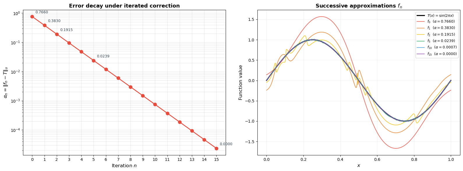
Initial error (alpha_0):  0.765964
Final error (alpha_15):  0.000023
Total reduction:          100.00%
Try it yourself –> UAT Contradiction Machine
What This Means#
Monico’s Theorem 3.4 establishes that \(\mathcal{N}_4\) – neural networks with 3 hidden layers and a 0-1 squashing activation – is dense in \(C(K)\). Here is how it fits into the broader landscape:
Monico’s theorem gives \(\mathcal{N}_4\) (3 hidden layers), while Cybenko’s theorem gives \(\mathcal{N}_2\) (1 hidden layer). The extra layers are the price paid for the elementary proof. Monico’s construction uses each layer for a specific purpose: Layer 1 separates points (Lemma 3.1), Layer 2 separates point from set (Lemma 3.2), Layer 3 separates set from set (Lemma 3.3).
Both theorems are existence results. They show approximation is possible but do not tell you how to find the weights. The proofs are non-constructive: they guarantee a network exists without providing an algorithm to compute it.
Neither theorem addresses learnability. Even though an approximating network exists, gradient descent might not find it. The gap between approximation theory and optimization is one of the deepest questions in deep learning.
For the limitations of the UAT (width explosion, curse of dimensionality, non-learnability), see Chapter 19, Section 19.4.
Exercises#
Exercise 3.1. The proof uses \(4\alpha/3\) as the upper bound on \(\|\hat{f} - T\|_u\). What if we used \(3\alpha/2\) instead? Rewrite the definitions of \(U^+\) and \(U^-\) (with \(\alpha/3\) replaced by an appropriate threshold), redo the three-case analysis, and find what \(\varepsilon\) must be in the application of Lemma 3.3. Does the proof still work?
Hint
With \(\delta = \alpha/2\) you get \(\|\hat{f} - T\|_u < 3\alpha/2\). Define \(U^+ = \{x : \alpha/2 \le (\hat{f} - T)(x) \le 3\alpha/2\}\). You will need \(H < \varepsilon\) on \(U^-\) and \(H > 1 - \varepsilon\) on \(U^+\). Work out the cases to find what value of \(\varepsilon\) makes all three inequalities strict.
Exercise 3.2. The proof constructs one improved \(f\) and derives a contradiction. What if we iterated the improvement, as in the numerical demonstration above? Does \(\|f_n - T\| \to 0\)? Why or why not?
Hint
The proof guarantees \(\alpha_{n+1} < \alpha_n\) at each step, so the sequence \((\alpha_n)\) is strictly decreasing and bounded below by \(0\). It therefore converges. But does it converge to \(0\)? Think about whether the reduction ratio \(\alpha_{n+1}/\alpha_n\) is bounded away from \(1\).
Exercise 3.3. \(\star\) Show explicitly that \(f = \hat{f} - \alpha H + \alpha/2 \in \mathcal{N}_4\) by counting layers. If \(\hat{f} \in \mathcal{N}_4\) uses \(m\) neurons in its hidden layers and \(H \in \mathcal{N}_3^\sigma\) uses \(p\) neurons, how many neurons does \(f\) require?
Hint
\(H \in \mathcal{N}_3^\sigma \subset \mathcal{N}_4\), so \(H\) can be written as an \(\mathcal{N}_4\) function. The function \(f = \hat{f} - \alpha H + \alpha/2\) is an affine combination of two \(\mathcal{N}_4\) elements. Count the neurons by tracing through the \(\mathcal{N}_k\) definitions – the neurons from \(\hat{f}\) and \(H\) are combined in the final affine layer.
Exercise 3.4. \(\star\star\) Implement the constructive version: given a target function \(T\) on \([0, 1]\) and a tolerance \(\varepsilon > 0\), build \(f \in \mathcal{N}_4\) achieving \(\|f - T\|_u < \varepsilon\). How many neurons do you need as a function of \(\varepsilon\)? Experiment with \(T(x) = \sin(2\pi x)\), \(T(x) = |x - 1/2|\), and \(T(x) = x^2\) for \(\varepsilon \in \{0.1, 0.01, 0.001\}\).
Hint
One approach: implement the iterative correction from the proof directly. At each step, build \(H\) as an explicit sum of sigmoids (as in Lemma 3.3). Track the total neuron count. You should observe that the number of neurons grows roughly as \(O(1/\varepsilon)\) or worse – this is the “width explosion” discussed in Chapter 19.