Chapter 18: Implementing Backpropagation from Scratch#
In this chapter, we translate the theory of Chapter 16 into working code. We build a
complete NeuralNetwork class using only NumPy, verify the gradients numerically, and
demonstrate the network’s ability to learn several non-trivial tasks: XOR, circular
decision boundaries, and function approximation.
import numpy as np
import matplotlib.pyplot as plt


class NeuralNetwork:
    """A complete feedforward neural network with backpropagation.

    Implements the four fundamental equations (BP1-BP4) from Chapter 16.
    """

    def __init__(self, layer_sizes, activation='sigmoid'):
        """
        Parameters
        ----------
        layer_sizes : list of int
            Number of neurons in each layer, e.g. [2, 4, 1] for
            2 inputs, 4 hidden neurons, 1 output.
        activation : str
            'sigmoid' or 'relu'
        """
        self.layer_sizes = layer_sizes
        self.L = len(layer_sizes) - 1  # number of weight layers
        self.activation_name = activation

        # Xavier initialization
        self.weights = []
        self.biases = []
        for l in range(self.L):
            n_in = layer_sizes[l]
            n_out = layer_sizes[l + 1]
            # Xavier: Var = 2 / (n_in + n_out)
            W = np.random.randn(n_out, n_in) * np.sqrt(2.0 / (n_in + n_out))
            b = np.zeros((n_out, 1))
            self.weights.append(W)
            self.biases.append(b)

        # Cache for forward pass (needed by backward pass)
        self.z_cache = []  # pre-activations
        self.a_cache = []  # activations

    def _activation(self, z):
        if self.activation_name == 'sigmoid':
            return 1.0 / (1.0 + np.exp(-np.clip(z, -500, 500)))
        elif self.activation_name == 'relu':
            return np.maximum(0, z)

    def _activation_derivative(self, z):
        if self.activation_name == 'sigmoid':
            s = self._activation(z)
            return s * (1 - s)
        elif self.activation_name == 'relu':
            return (z > 0).astype(float)

    def forward(self, X):
        """Forward pass through the network.

        Parameters
        ----------
        X : ndarray, shape (n_features, n_samples)
            Input data (each column is a sample).

        Returns
        -------
        a : ndarray, shape (n_outputs, n_samples)
            Network output.
        """
        self.z_cache = []
        self.a_cache = [X]  # a^(0) = input

        a = X
        for l in range(self.L):
            z = self.weights[l] @ a + self.biases[l]
            a = self._activation(z)
            self.z_cache.append(z)
            self.a_cache.append(a)

        return a

    def compute_loss(self, y_hat, Y):
        """Compute MSE loss: L = (1/2m) * sum(||y_hat - Y||^2)

        Parameters
        ----------
        y_hat : ndarray, shape (n_outputs, n_samples)
        Y : ndarray, shape (n_outputs, n_samples)

        Returns
        -------
        loss : float
        """
        m = Y.shape[1]
        return 0.5 * np.sum((y_hat - Y)**2) / m

    def backward(self, Y):
        """Backward pass: compute gradients using BP1-BP4.

        Parameters
        ----------
        Y : ndarray, shape (n_outputs, n_samples)
            Target values.

        Returns
        -------
        dW : list of ndarray
            Weight gradients for each layer.
        db : list of ndarray
            Bias gradients for each layer.
        """
        m = Y.shape[1]
        dW = [None] * self.L
        db = [None] * self.L

        # BP1: Output layer error
        # dL/da^(L) for MSE = (a^(L) - Y) / m
        a_L = self.a_cache[-1]
        dL_da = (a_L - Y) / m
        sigma_prime = self._activation_derivative(self.z_cache[-1])
        delta = dL_da * sigma_prime

        # BP3 and BP4 for output layer
        dW[-1] = delta @ self.a_cache[-2].T  # BP3
        db[-1] = np.sum(delta, axis=1, keepdims=True)  # BP4

        # BP2: Backpropagate through hidden layers
        for l in range(self.L - 2, -1, -1):
            sigma_prime = self._activation_derivative(self.z_cache[l])
            delta = (self.weights[l + 1].T @ delta) * sigma_prime  # BP2
            dW[l] = delta @ self.a_cache[l].T  # BP3
            db[l] = np.sum(delta, axis=1, keepdims=True)  # BP4

        return dW, db

    def update(self, dW, db, eta):
        """Update parameters using gradient descent.

        Parameters
        ----------
        dW, db : gradients from backward()
        eta : float, learning rate
        """
        for l in range(self.L):
            self.weights[l] -= eta * dW[l]
            self.biases[l] -= eta * db[l]

    def train(self, X, Y, epochs, eta, batch_size=None, verbose=True):
        """Full training loop.

        Parameters
        ----------
        X : ndarray, shape (n_features, n_samples)
        Y : ndarray, shape (n_outputs, n_samples)
        epochs : int
        eta : float, learning rate
        batch_size : int or None (full batch if None)
        verbose : bool

        Returns
        -------
        loss_history : list of float
        """
        m = X.shape[1]
        if batch_size is None:
            batch_size = m

        loss_history = []

        for epoch in range(epochs):
            # Shuffle
            perm = np.random.permutation(m)
            X_shuffled = X[:, perm]
            Y_shuffled = Y[:, perm]

            for start in range(0, m, batch_size):
                end = min(start + batch_size, m)
                X_batch = X_shuffled[:, start:end]
                Y_batch = Y_shuffled[:, start:end]

                # Forward
                y_hat = self.forward(X_batch)

                # Backward
                dW, db = self.backward(Y_batch)

                # Update
                self.update(dW, db, eta)

            # Track loss on full dataset
            y_hat_full = self.forward(X)
            loss = self.compute_loss(y_hat_full, Y)
            loss_history.append(loss)

            if verbose and (epoch % (epochs // 10) == 0 or epoch == epochs - 1):
                print(f"Epoch {epoch:5d}/{epochs}: Loss = {loss:.6f}")

        return loss_history


print("NeuralNetwork class defined successfully.")
print("Methods: __init__, forward, compute_loss, backward, update, train")
NeuralNetwork class defined successfully.
Methods: __init__, forward, compute_loss, backward, update, train
18.1 Gradient Checking#
Before trusting our backpropagation implementation, we must verify it numerically.
Algorithm (Numerical Gradient Checking)
Goal: Verify that the analytically computed gradient (from backpropagation) matches the numerically computed gradient (from finite differences).
For each parameter \(\theta_i\) in the network:
Compute the analytical gradient \(g_i = \frac{\partial \mathcal{L}}{\partial \theta_i}\) using backpropagation
Compute the numerical gradient using the two-sided finite difference:
Compute the relative error:
where \(\delta \approx 10^{-8}\) prevents division by zero.
Pass criterion: relative error \(< 10^{-7}\) for correct implementation.
Danger
❗ ALWAYS verify your gradient implementation numerically before training. A wrong gradient will silently produce bad results – the network will still “train” but learn nonsense. Gradient bugs are insidious because the loss may still decrease (just not as well as it should), making the error hard to detect from loss curves alone.
Tip
Use \(\varepsilon \approx 10^{-7}\) for numerical gradient checking. Too small (e.g., \(10^{-15}\)) and floating-point rounding errors dominate. Too large (e.g., \(10^{-2}\)) and the finite-difference approximation is poor. The sweet spot is \(10^{-7}\) to \(10^{-5}\).
Warning
Gradient checking is \(O(n)\) forward passes per parameter – for a network with \(P\) total parameters, gradient checking requires \(2P\) forward passes. This makes it far too slow for production training. Only use it during development to verify correctness, then disable it for actual training.
Tip
Relative error interpretation: \(< 10^{-7}\): perfect, your implementation is correct. \(10^{-5}\) to \(10^{-7}\): acceptable, might be OK. \(> 10^{-3}\): something is wrong, debug your backprop.
Show code cell source
# Gradient Checking

import numpy as np

np.random.seed(42)

# Small network for gradient checking
nn_check = NeuralNetwork([3, 4, 2], activation='sigmoid')

# Random data
X_check = np.random.randn(3, 5)
Y_check = np.random.randn(2, 5)

# Get analytical gradients
y_hat = nn_check.forward(X_check)
dW_analytical, db_analytical = nn_check.backward(Y_check)

# Numerical gradient checking
epsilon = 1e-7
max_rel_error = 0

print("Gradient Checking Results:")
print("=" * 60)

for l in range(nn_check.L):
    # Check weights
    dW_numerical = np.zeros_like(nn_check.weights[l])
    for i in range(nn_check.weights[l].shape[0]):
        for j in range(nn_check.weights[l].shape[1]):
            # f(theta + epsilon)
            nn_check.weights[l][i, j] += epsilon
            y_plus = nn_check.forward(X_check)
            loss_plus = nn_check.compute_loss(y_plus, Y_check)

            # f(theta - epsilon)
            nn_check.weights[l][i, j] -= 2 * epsilon
            y_minus = nn_check.forward(X_check)
            loss_minus = nn_check.compute_loss(y_minus, Y_check)

            # Restore
            nn_check.weights[l][i, j] += epsilon

            dW_numerical[i, j] = (loss_plus - loss_minus) / (2 * epsilon)

    # Relative error
    diff = np.linalg.norm(dW_analytical[l] - dW_numerical)
    norm_sum = np.linalg.norm(dW_analytical[l]) + np.linalg.norm(dW_numerical)
    rel_error = diff / (norm_sum + 1e-8)
    max_rel_error = max(max_rel_error, rel_error)

    print(f"Layer {l+1} weights: relative error = {rel_error:.2e}", end="")
    print("  [OK]" if rel_error < 1e-5 else "  [FAIL]")

    # Check biases
    db_numerical = np.zeros_like(nn_check.biases[l])
    for i in range(nn_check.biases[l].shape[0]):
        nn_check.biases[l][i, 0] += epsilon
        y_plus = nn_check.forward(X_check)
        loss_plus = nn_check.compute_loss(y_plus, Y_check)

        nn_check.biases[l][i, 0] -= 2 * epsilon
        y_minus = nn_check.forward(X_check)
        loss_minus = nn_check.compute_loss(y_minus, Y_check)

        nn_check.biases[l][i, 0] += epsilon

        db_numerical[i, 0] = (loss_plus - loss_minus) / (2 * epsilon)

    diff_b = np.linalg.norm(db_analytical[l] - db_numerical)
    norm_sum_b = np.linalg.norm(db_analytical[l]) + np.linalg.norm(db_numerical)
    rel_error_b = diff_b / (norm_sum_b + 1e-8)
    max_rel_error = max(max_rel_error, rel_error_b)

    print(f"Layer {l+1} biases:  relative error = {rel_error_b:.2e}", end="")
    print("  [OK]" if rel_error_b < 1e-5 else "  [FAIL]")

print("=" * 60)
print(f"Maximum relative error: {max_rel_error:.2e}")
if max_rel_error < 1e-5:
    print("GRADIENT CHECK PASSED")
else:
    print("GRADIENT CHECK FAILED")
Gradient Checking Results:
============================================================
Layer 1 weights: relative error = 4.22e-08  [OK]
Layer 1 biases:  relative error = 1.03e-08  [OK]
Layer 2 weights: relative error = 6.99e-09  [OK]
Layer 2 biases:  relative error = 2.67e-09  [OK]
============================================================
Maximum relative error: 4.22e-08
GRADIENT CHECK PASSED
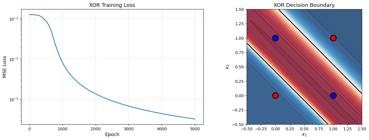
18.2 Demo 1: Learning XOR#
The XOR problem is the classic test case for multilayer networks. Recall that a single perceptron cannot solve XOR (Minsky & Papert, 1969), but a network with one hidden layer can.
Show code cell source
# Demo 1: Learning XOR

import numpy as np
import matplotlib.pyplot as plt

np.random.seed(42)

# XOR data
X_xor = np.array([[0, 0, 1, 1],
                   [0, 1, 0, 1]], dtype=float)  # 2x4
Y_xor = np.array([[0, 1, 1, 0]], dtype=float)   # 1x4

# Network: 2 -> 4 -> 1, sigmoid
nn_xor = NeuralNetwork([2, 4, 1], activation='sigmoid')

print("Training on XOR...")
print(f"Network architecture: 2 -> 4 -> 1 (sigmoid)")
print(f"Learning rate: 2.0, Epochs: 5000")
print()

loss_history = nn_xor.train(X_xor, Y_xor, epochs=5000, eta=2.0, verbose=True)

# Final predictions
print("\nFinal Predictions:")
y_pred = nn_xor.forward(X_xor)
for i in range(4):
    print(f"  Input: ({X_xor[0,i]:.0f}, {X_xor[1,i]:.0f}) -> "
          f"Predicted: {y_pred[0,i]:.4f}, Target: {Y_xor[0,i]:.0f}")

# Plot loss curve and decision boundary
fig, axes = plt.subplots(1, 2, figsize=(14, 5))

# Loss curve
axes[0].plot(loss_history, linewidth=2, color='#2E86C1')
axes[0].set_xlabel('Epoch', fontsize=12)
axes[0].set_ylabel('MSE Loss', fontsize=12)
axes[0].set_title('XOR Training Loss', fontsize=13)
axes[0].set_yscale('log')
axes[0].grid(True, alpha=0.3)

# Decision boundary
xx, yy = np.meshgrid(np.linspace(-0.5, 1.5, 200), np.linspace(-0.5, 1.5, 200))
grid = np.c_[xx.ravel(), yy.ravel()].T  # 2 x N
z_grid = nn_xor.forward(grid)
z_grid = z_grid.reshape(xx.shape)

axes[1].contourf(xx, yy, z_grid, levels=50, cmap='RdBu_r', alpha=0.8)
axes[1].contour(xx, yy, z_grid, levels=[0.5], colors='black', linewidths=2)
# Plot data points
for i in range(4):
    color = 'red' if Y_xor[0, i] == 0 else 'blue'
    axes[1].scatter(X_xor[0, i], X_xor[1, i], c=color, s=200,
                    edgecolors='black', linewidth=2, zorder=5)
axes[1].set_xlabel('$x_1$', fontsize=12)
axes[1].set_ylabel('$x_2$', fontsize=12)
axes[1].set_title('XOR Decision Boundary', fontsize=13)
axes[1].set_aspect('equal')

plt.tight_layout()
plt.savefig('xor_learning.png', dpi=150, bbox_inches='tight')
plt.show()
Training on XOR...
Network architecture: 2 -> 4 -> 1 (sigmoid)
Learning rate: 2.0, Epochs: 5000

Epoch     0/5000: Loss = 0.126088
Epoch   500/5000: Loss = 0.086947
Epoch  1000/5000: Loss = 0.008075
Epoch  1500/5000: Loss = 0.002480
Epoch  2000/5000: Loss = 0.001353
Epoch  2500/5000: Loss = 0.000906
Epoch  3000/5000: Loss = 0.000673
Epoch  3500/5000: Loss = 0.000532
Epoch  4000/5000: Loss = 0.000438
Epoch  4500/5000: Loss = 0.000371
Epoch  4999/5000: Loss = 0.000321

Final Predictions:
  Input: (0, 0) -> Predicted: 0.0288, Target: 0
  Input: (0, 1) -> Predicted: 0.9756, Target: 1
  Input: (1, 0) -> Predicted: 0.9763, Target: 1
  Input: (1, 1) -> Predicted: 0.0242, Target: 0
18.3 Demo 2: Learning a Circle#
Can the network learn to classify points inside vs. outside a circle? This requires a nonlinear, closed decision boundary.
Show code cell source
# Demo 2: Learning a Circle

import numpy as np
import matplotlib.pyplot as plt

np.random.seed(42)

# Generate data: inside/outside a circle of radius 0.5
n_samples = 500
X_circle = np.random.uniform(-1, 1, (2, n_samples))
Y_circle = ((X_circle[0]**2 + X_circle[1]**2) < 0.5**2).astype(float).reshape(1, -1)

print(f"Circle dataset: {n_samples} points")
print(f"  Inside circle: {int(Y_circle.sum())}")
print(f"  Outside circle: {n_samples - int(Y_circle.sum())}")

# Network: 2 -> 8 -> 1
nn_circle = NeuralNetwork([2, 8, 1], activation='sigmoid')

loss_hist = nn_circle.train(X_circle, Y_circle, epochs=3000, eta=5.0, verbose=True)

# Plot
fig, axes = plt.subplots(1, 3, figsize=(18, 5))

# Loss curve
axes[0].plot(loss_hist, linewidth=2, color='#2E86C1')
axes[0].set_xlabel('Epoch', fontsize=12)
axes[0].set_ylabel('MSE Loss', fontsize=12)
axes[0].set_title('Circle Classification: Training Loss', fontsize=13)
axes[0].set_yscale('log')
axes[0].grid(True, alpha=0.3)

# Data
colors = ['red' if y == 0 else 'blue' for y in Y_circle[0]]
axes[1].scatter(X_circle[0], X_circle[1], c=colors, s=15, alpha=0.5)
theta = np.linspace(0, 2*np.pi, 100)
axes[1].plot(0.5*np.cos(theta), 0.5*np.sin(theta), 'k--', linewidth=2, label='True boundary')
axes[1].set_xlabel('$x_1$', fontsize=12)
axes[1].set_ylabel('$x_2$', fontsize=12)
axes[1].set_title('Training Data', fontsize=13)
axes[1].set_aspect('equal')
axes[1].legend()

# Decision boundary
xx, yy = np.meshgrid(np.linspace(-1, 1, 200), np.linspace(-1, 1, 200))
grid = np.c_[xx.ravel(), yy.ravel()].T
z_grid = nn_circle.forward(grid).reshape(xx.shape)

axes[2].contourf(xx, yy, z_grid, levels=50, cmap='RdBu_r', alpha=0.8)
axes[2].contour(xx, yy, z_grid, levels=[0.5], colors='black', linewidths=2)
axes[2].plot(0.5*np.cos(theta), 0.5*np.sin(theta), 'g--', linewidth=2, label='True boundary')
axes[2].set_xlabel('$x_1$', fontsize=12)
axes[2].set_ylabel('$x_2$', fontsize=12)
axes[2].set_title('Learned Decision Boundary', fontsize=13)
axes[2].set_aspect('equal')
axes[2].legend()

plt.tight_layout()
plt.savefig('circle_learning.png', dpi=150, bbox_inches='tight')
plt.show()

# Accuracy
y_pred = nn_circle.forward(X_circle)
accuracy = np.mean((y_pred > 0.5).astype(float) == Y_circle)
print(f"\nTraining accuracy: {accuracy*100:.1f}%")
Circle dataset: 500 points
  Inside circle: 99
  Outside circle: 401
Epoch     0/3000: Loss = 0.080713
Epoch   300/3000: Loss = 0.079283
Epoch   600/3000: Loss = 0.079212
Epoch   900/3000: Loss = 0.078966
Epoch  1200/3000: Loss = 0.077210
Epoch  1500/3000: Loss = 0.065074
Epoch  1800/3000: Loss = 0.030372
Epoch  2100/3000: Loss = 0.018973
Epoch  2400/3000: Loss = 0.015537
Epoch  2700/3000: Loss = 0.013791
Epoch 2999/3000: Loss = 0.012668
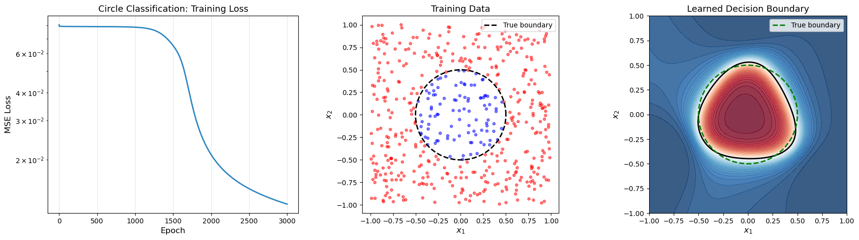
Training accuracy: 97.8%
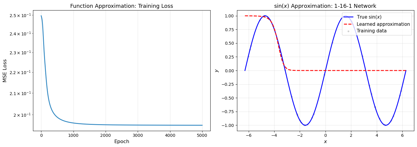
18.4 Demo 3: Function Approximation#
We approximate the function \(\sin(x)\) using a neural network with a single hidden layer. This previews the Universal Approximation Theorem (Chapter 19).
Show code cell source
# Demo 3: Approximating sin(x)

import numpy as np
import matplotlib.pyplot as plt

np.random.seed(42)

# Training data
n_train = 200
X_sin = np.random.uniform(-2*np.pi, 2*np.pi, (1, n_train))
Y_sin = np.sin(X_sin)

# Normalize inputs to [-1, 1] for better training
X_norm = X_sin / (2 * np.pi)

# Network: 1 -> 16 -> 1
nn_sin = NeuralNetwork([1, 16, 1], activation='sigmoid')

print("Approximating sin(x) with a 1->16->1 network...")
loss_hist = nn_sin.train(X_norm, Y_sin, epochs=5000, eta=5.0, verbose=True)

# Plot
fig, axes = plt.subplots(1, 2, figsize=(14, 5))

# Loss curve
axes[0].plot(loss_hist, linewidth=2, color='#2E86C1')
axes[0].set_xlabel('Epoch', fontsize=12)
axes[0].set_ylabel('MSE Loss', fontsize=12)
axes[0].set_title('Function Approximation: Training Loss', fontsize=13)
axes[0].set_yscale('log')
axes[0].grid(True, alpha=0.3)

# Learned function vs true
x_test = np.linspace(-2*np.pi, 2*np.pi, 500).reshape(1, -1)
x_test_norm = x_test / (2 * np.pi)
y_learned = nn_sin.forward(x_test_norm)

axes[1].plot(x_test[0], np.sin(x_test[0]), 'b-', linewidth=2, label='True $\\sin(x)$')
axes[1].plot(x_test[0], y_learned[0], 'r--', linewidth=2, label='Learned approximation')
axes[1].scatter(X_sin[0, ::5], Y_sin[0, ::5], s=10, alpha=0.3, color='gray', label='Training data')
axes[1].set_xlabel('$x$', fontsize=12)
axes[1].set_ylabel('$y$', fontsize=12)
axes[1].set_title('$\\sin(x)$ Approximation: 1-16-1 Network', fontsize=13)
axes[1].legend(fontsize=11)
axes[1].grid(True, alpha=0.3)

plt.tight_layout()
plt.savefig('sin_approximation.png', dpi=150, bbox_inches='tight')
plt.show()
Approximating sin(x) with a 1->16->1 network...
Epoch     0/5000: Loss = 0.249646
Epoch   500/5000: Loss = 0.198892
Epoch  1000/5000: Loss = 0.196333
Epoch  1500/5000: Loss = 0.195760
Epoch  2000/5000: Loss = 0.195559
Epoch  2500/5000: Loss = 0.195469
Epoch  3000/5000: Loss = 0.195423
Epoch  3500/5000: Loss = 0.195395
Epoch  4000/5000: Loss = 0.195377
Epoch  4500/5000: Loss = 0.195362
Epoch  4999/5000: Loss = 0.195351
18.5 Hyperparameter Exploration#
The performance of a neural network depends heavily on hyperparameters. Here we explore the effect of hidden layer size, learning rate, and number of epochs on the XOR task.
Show code cell source
# Hyperparameter exploration on XOR

import numpy as np
import matplotlib.pyplot as plt

X_xor = np.array([[0, 0, 1, 1],
                   [0, 1, 0, 1]], dtype=float)
Y_xor = np.array([[0, 1, 1, 0]], dtype=float)

fig, axes = plt.subplots(1, 3, figsize=(18, 5))

# (1) Effect of hidden layer size
hidden_sizes = [2, 3, 4, 8, 16]
for h in hidden_sizes:
    np.random.seed(42)
    nn = NeuralNetwork([2, h, 1], activation='sigmoid')
    losses = nn.train(X_xor, Y_xor, epochs=3000, eta=2.0, verbose=False)
    axes[0].plot(losses, label=f'H={h}', linewidth=1.5)
axes[0].set_xlabel('Epoch', fontsize=12)
axes[0].set_ylabel('MSE Loss', fontsize=12)
axes[0].set_title('Effect of Hidden Layer Size', fontsize=13)
axes[0].set_yscale('log')
axes[0].legend()
axes[0].grid(True, alpha=0.3)

# (2) Effect of learning rate
etas = [0.1, 0.5, 1.0, 2.0, 5.0]
for eta in etas:
    np.random.seed(42)
    nn = NeuralNetwork([2, 4, 1], activation='sigmoid')
    losses = nn.train(X_xor, Y_xor, epochs=3000, eta=eta, verbose=False)
    axes[1].plot(losses, label=f'$\\eta$={eta}', linewidth=1.5)
axes[1].set_xlabel('Epoch', fontsize=12)
axes[1].set_ylabel('MSE Loss', fontsize=12)
axes[1].set_title('Effect of Learning Rate', fontsize=13)
axes[1].set_yscale('log')
axes[1].legend()
axes[1].grid(True, alpha=0.3)

# (3) Final loss vs epochs (showing when XOR is "solved")
epoch_counts = [100, 500, 1000, 2000, 5000, 10000]
final_losses = []
for ep in epoch_counts:
    np.random.seed(42)
    nn = NeuralNetwork([2, 4, 1], activation='sigmoid')
    losses = nn.train(X_xor, Y_xor, epochs=ep, eta=2.0, verbose=False)
    final_losses.append(losses[-1])

axes[2].bar(range(len(epoch_counts)), final_losses, color='steelblue', edgecolor='black')
axes[2].set_xticks(range(len(epoch_counts)))
axes[2].set_xticklabels([str(e) for e in epoch_counts])
axes[2].set_xlabel('Number of Epochs', fontsize=12)
axes[2].set_ylabel('Final MSE Loss', fontsize=12)
axes[2].set_title('Final Loss vs Training Duration', fontsize=13)
axes[2].set_yscale('log')
axes[2].grid(True, alpha=0.3, axis='y')

plt.tight_layout()
plt.savefig('hyperparameter_exploration.png', dpi=150, bbox_inches='tight')
plt.show()

Decision Boundary Evolution#
The following visualization shows how the decision boundary for the circle classification task evolves during training, demonstrating the gradual refinement of the learned representation.
Show code cell source
import numpy as np
import matplotlib.pyplot as plt

np.random.seed(42)

# Generate circle data
n_samples = 500
X_circle = np.random.uniform(-1, 1, (2, n_samples))
Y_circle = ((X_circle[0]**2 + X_circle[1]**2) < 0.5**2).astype(float).reshape(1, -1)

# Network: 2 -> 8 -> 1
nn_evo = NeuralNetwork([2, 8, 1], activation='sigmoid')

# Grid for decision boundary
xx, yy = np.meshgrid(np.linspace(-1.2, 1.2, 150), np.linspace(-1.2, 1.2, 150))
grid = np.c_[xx.ravel(), yy.ravel()].T

# Snapshot epochs
snapshot_epochs = [0, 50, 200, 500, 1000, 3000]
fig, axes = plt.subplots(2, 3, figsize=(16, 10))
axes = axes.flatten()

epoch_counter = 0
snapshot_idx = 0

# True boundary
theta_circle = np.linspace(0, 2*np.pi, 100)

# Snapshot at epoch 0
z_grid = nn_evo.forward(grid).reshape(xx.shape)
axes[0].contourf(xx, yy, z_grid, levels=50, cmap='RdBu_r', alpha=0.8)
axes[0].contour(xx, yy, z_grid, levels=[0.5], colors='black', linewidths=2)
axes[0].plot(0.5*np.cos(theta_circle), 0.5*np.sin(theta_circle), 'g--', linewidth=2)
for i in range(n_samples):
    color = 'red' if Y_circle[0, i] == 0 else 'blue'
    axes[0].scatter(X_circle[0, i], X_circle[1, i], c=color, s=5, alpha=0.3)
axes[0].set_title('Epoch 0 (random init)', fontsize=12)
axes[0].set_aspect('equal')
axes[0].set_xlim(-1.2, 1.2)
axes[0].set_ylim(-1.2, 1.2)
axes[0].grid(True, alpha=0.1)

# Train and snapshot
m = X_circle.shape[1]
eta = 5.0
current_epoch = 0

for panel_idx, target_epoch in enumerate(snapshot_epochs[1:], 1):
    # Train from current_epoch to target_epoch
    epochs_to_run = target_epoch - current_epoch
    for ep in range(epochs_to_run):
        perm = np.random.permutation(m)
        X_s = X_circle[:, perm]
        Y_s = Y_circle[:, perm]
        y_hat = nn_evo.forward(X_s)
        dW, db = nn_evo.backward(Y_s)
        nn_evo.update(dW, db, eta)
    current_epoch = target_epoch

    # Snapshot
    z_grid = nn_evo.forward(grid).reshape(xx.shape)
    axes[panel_idx].contourf(xx, yy, z_grid, levels=50, cmap='RdBu_r', alpha=0.8)
    axes[panel_idx].contour(xx, yy, z_grid, levels=[0.5], colors='black', linewidths=2)
    axes[panel_idx].plot(0.5*np.cos(theta_circle), 0.5*np.sin(theta_circle), 'g--', linewidth=2)
    for i in range(n_samples):
        color = 'red' if Y_circle[0, i] == 0 else 'blue'
        axes[panel_idx].scatter(X_circle[0, i], X_circle[1, i], c=color, s=5, alpha=0.3)

    # Compute accuracy
    y_pred_snap = nn_evo.forward(X_circle)
    acc_snap = np.mean((y_pred_snap > 0.5).astype(float) == Y_circle) * 100
    loss_snap = nn_evo.compute_loss(y_pred_snap, Y_circle)

    axes[panel_idx].set_title(f'Epoch {target_epoch} (acc={acc_snap:.0f}%, loss={loss_snap:.4f})', fontsize=12)
    axes[panel_idx].set_aspect('equal')
    axes[panel_idx].set_xlim(-1.2, 1.2)
    axes[panel_idx].set_ylim(-1.2, 1.2)
    axes[panel_idx].grid(True, alpha=0.1)

plt.suptitle('Decision Boundary Evolution During Training', fontsize=15, fontweight='bold')
plt.tight_layout()
plt.savefig('decision_boundary_evolution.png', dpi=150, bbox_inches='tight')
plt.show()

print("The decision boundary evolves from random (epoch 0) to an increasingly")
print("accurate approximation of the true circular boundary.")
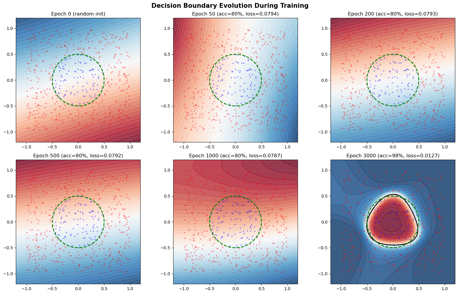
The decision boundary evolves from random (epoch 0) to an increasingly
accurate approximation of the true circular boundary.
Exercises#
Exercise 18.1. Extend the NeuralNetwork class to support tanh activation. Verify the
gradient with gradient checking. Compare sigmoid vs tanh on the XOR problem.
Exercise 18.2. Implement L2 regularization (weight decay). Add a term \(\frac{\lambda}{2}\sum_{l} \|\mathbf{W}^{(l)}\|_F^2\) to the loss, and modify the gradient accordingly. Test on the circle problem and observe the effect on the decision boundary.
Exercise 18.3. Train a network to learn the function \(f(x) = x^2\) on \([-2, 2]\). Experiment with different architectures (1-8-1, 1-16-1, 1-8-8-1). Which works best?
Exercise 18.4. Implement momentum in the update method. Compare convergence
with and without momentum (\(\beta = 0.9\)) on all three demos.
Exercise 18.5. Generate a two-spirals dataset (two interleaved spirals). This is a much harder classification problem. Determine the minimum network architecture needed to solve it.