Chapter 40: Attention Is All You Need

This is it — the synthesis chapter. You have built every component you need:

• scaled dot-product attention (Chapter 38) and multi-head self-attention (Chapter 39);

• encoder-decoder sequence transduction (Chapter 36);

• cross-entropy loss (Chapter 26), Adam (Chapter 27), PyTorch nn.Module (Chapter 29);

• residual connections as a fix for vanishing gradients (Chapters 17, 34).

We assemble all of these into the complete Transformer of Vaswani et al. (2017), and train one on the same string-reversal task you have been chasing since Chapter 36. By the end you will be able to read the original Attention Is All You Need paper and recognise every line.

Original paper: Vaswani, Shazeer, Parmar, Uszkoreit, Jones, Gomez, Kaiser, Polosukhin. Attention Is All You Need. NeurIPS 2017 (arXiv:1706.03762).

40.1 The Big Picture

The Transformer is two stacks of identical blocks: an encoder that reads the source and a decoder that writes the target. Each encoder block does:

\[ x \;\to\; \mathrm{LN}(x + \mathrm{MHA}(x)) \;\to\; \mathrm{LN}(\cdot + \mathrm{FFN}(\cdot)) \]

Each decoder block does the same plus a cross-attention sub-layer that lets the decoder attend to the encoder output:

\[ x \;\to\; \mathrm{LN}(x + \mathrm{MHA}_\text{causal}(x)) \;\to\; \mathrm{LN}(\cdot + \mathrm{MHA}_\text{cross}(\cdot, \mathrm{enc}, \mathrm{enc})) \;\to\; \mathrm{LN}(\cdot + \mathrm{FFN}(\cdot)) \]

Decoding the abbreviations

The equations above use compact names for sub-layers. Here is what each one does, where you have already met it, and how it appears in the code in section 40.6.

Symbol	Full name	What it does	Built in chapter	Class / call in code
\(\mathrm{LN}(\cdot)\)	Layer Normalisation	Normalises each token’s feature vector to mean 0, variance 1, then scales/shifts. Stabilises training.	§40.3 (this chapter)	nn.LayerNorm(d_model) — used as self.ln1, self.ln2, self.ln3
\(\mathrm{MHA}(x)\)	Multi-Head Self-Attention	Each token attends to every other token in the same sequence using \(h\) parallel attention heads. Inputs Q, K, V all come from \(x\).	Ch. 39	MultiHeadAttention(d_model, n_heads) called as self.mha(x, x, x, mask)
\(\mathrm{MHA}_\text{causal}(x)\)	Causally-Masked MHA	Same as MHA, but the attention mask zeros out future positions so token \(i\) cannot peek at \(i{+}1, i{+}2, \ldots\) — required during training of the decoder.	§40.5 (mask) + Ch. 39	self.mha(x, x, x, causal_mask) (same class, different mask)
\(\mathrm{MHA}_\text{cross}(x, \mathrm{enc}, \mathrm{enc})\)	Cross-Attention	Same MHA machinery, but Q comes from the decoder and K, V come from the encoder output. This is exactly Bahdanau attention generalised to multiple heads.	Ch. 37 (Bahdanau) → multi-head form in §40.6	self.mha_cross(dec, enc, enc, src_mask)
\(\mathrm{FFN}(\cdot)\)	Position-wise Feed-Forward Network	A 2-layer MLP Linear → ReLU → Linear applied independently to every token. Lets the model do per-token nonlinear processing between attention layers.	§40.6 (FeedForward class)	FeedForward(d_model, d_ff)
\(x + \mathrm{Sublayer}(x)\)	Residual connection	The input is added to the sub-layer’s output before normalising. Keeps gradients flowing through deep stacks (callback to ResNets in CNN chapters).	§40.4	the + x term inside each block’s forward()
\(\mathrm{enc}\)	encoder output tensor	The final \((B, T_\text{src}, d_\text{model})\) representation produced by the encoder stack. The decoder reads this through cross-attention.	output of Transformer.encode()	enc_out

Reading rule. Whenever you see a stack of \(\mathrm{LN}(x + \text{Something}(x))\), read it as: “do the sub-layer, add the input back (residual), normalise.” Every encoder block has two such stacks (MHA, FFN); every decoder block has three (causal MHA, cross-attention, FFN).

Three new ingredients

Three new ingredients appear that you have not built before:

1. Positional encoding — because self-attention is permutation-equivariant (Exercise 39.1).

2. Layer normalisation — a per-token cousin of batch norm.

3. Causal masking — the decoder cannot peek at future tokens during training.

Sections 40.2–40.5 develop each ingredient. Section 40.6 puts it all together. Section 40.7 trains the model. Section 40.8 visualises the heads.

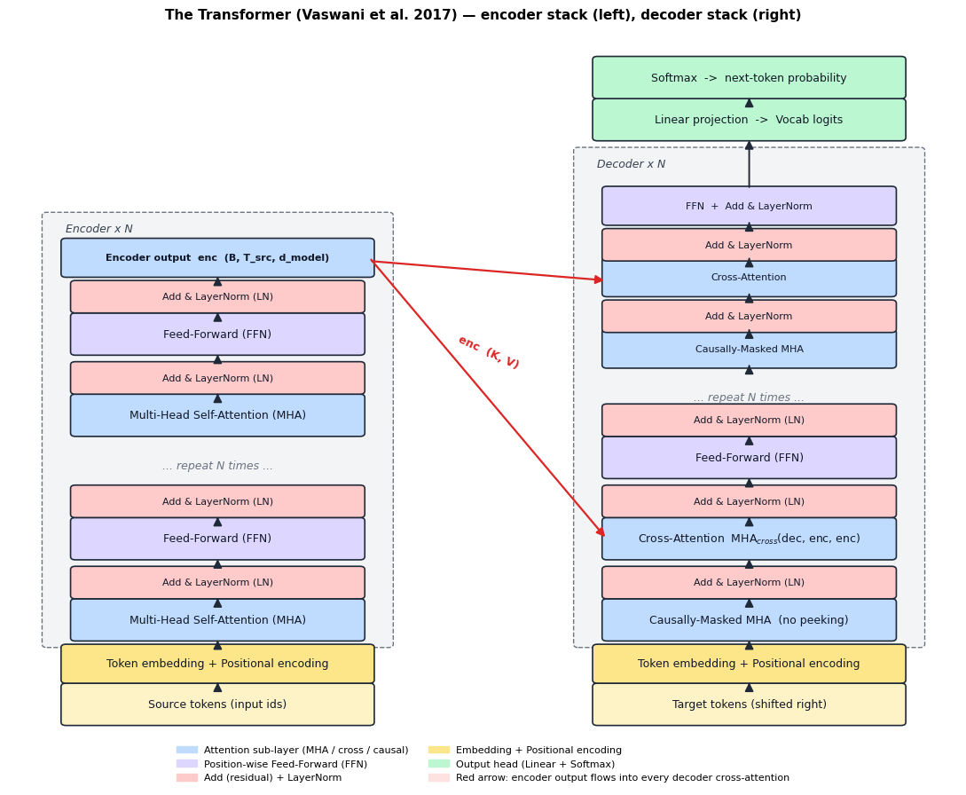
A picture of the whole machine

Before diving into ingredient-by-ingredient (positional encoding, layer norm, masking) it helps to see the full architecture once. The diagram below shows what we are building: an encoder stack and a decoder stack, with the encoder output piped into every decoder layer through cross-attention.

Keep this picture in mind as we build each block in §40.2–§40.6.

Show code cell source Hide code cell source

import sys, os; sys.path.insert(0, os.path.abspath('.'))
import math, random
import torch
import torch.nn as nn
import torch.nn.functional as F
import numpy as np
import matplotlib.pyplot as plt

from utils import (
    PAD, SOS, EOS, ITOS, STOI, VOCAB_SIZE,
    encode, decode, make_pair, make_batch, accuracy,
)

torch.manual_seed(0); random.seed(0)
device = torch.device('cpu')

Show code cell source Hide code cell source

# A schematic of the full Transformer (Vaswani et al. 2017): encoder stack on the left,
# decoder stack on the right, with cross-attention arrows connecting them.
import matplotlib.patches as mpatches
from matplotlib.patches import FancyArrowPatch, FancyBboxPatch

fig, ax = plt.subplots(figsize=(11, 9))
ax.set_xlim(0, 10); ax.set_ylim(0, 11)
ax.axis('off')

def block(x, y, w, h, label, color, fontsize=9, weight='normal'):
    box = FancyBboxPatch((x, y), w, h, boxstyle='round,pad=0.05',
                          facecolor=color, edgecolor='#1f2937', linewidth=1.2)
    ax.add_patch(box)
    ax.text(x + w/2, y + h/2, label, ha='center', va='center',
            fontsize=fontsize, weight=weight, color='#111827')

def arrow(x1, y1, x2, y2, color='#1f2937', style='-|>', lw=1.4):
    ax.add_patch(FancyArrowPatch((x1, y1), (x2, y2),
                                  arrowstyle=style, color=color,
                                  mutation_scale=14, lw=lw))

def residual(x_left, y_bot, y_top, x_right):
    # Curved residual line on the left of a sub-layer block
    ax.add_patch(FancyArrowPatch((x_left, y_bot), (x_right, y_top),
                                  connectionstyle='arc3,rad=-0.4',
                                  arrowstyle='-|>', color='#9ca3af',
                                  mutation_scale=10, lw=1.0, linestyle='--'))

# Colors
c_emb = '#fde68a'       # embeddings/positional
c_attn = '#bfdbfe'      # attention sublayers
c_ffn = '#ddd6fe'       # FFN
c_ln  = '#fecaca'       # layer norm
c_out = '#bbf7d0'       # output head
c_stack = '#f3f4f6'     # encoder/decoder enclosing rect

# ---------- ENCODER (left) ----------
# Outer "N x" box
ax.add_patch(FancyBboxPatch((0.4, 1.6), 3.6, 6.6, boxstyle='round,pad=0.05',
                             facecolor=c_stack, edgecolor='#6b7280',
                             linewidth=1.0, linestyle='--'))
ax.text(0.6, 7.95, 'Encoder x N', fontsize=9, color='#374151', style='italic')

# Encoder block stack: bottom -> top
block(0.6, 0.4, 3.2, 0.55, 'Source tokens (input ids)', '#fef3c7')
block(0.6, 1.05, 3.2, 0.5, 'Token embedding + Positional encoding', c_emb)
arrow(2.2, 0.95, 2.2, 1.05)

block(0.7, 1.7, 3.0, 0.55, 'Multi-Head Self-Attention (MHA)', c_attn)
arrow(2.2, 1.55, 2.2, 1.7)
block(0.7, 2.35, 3.0, 0.4, 'Add & LayerNorm (LN)', c_ln, fontsize=8)
arrow(2.2, 2.25, 2.2, 2.35)

block(0.7, 2.95, 3.0, 0.55, 'Feed-Forward (FFN)', c_ffn)
arrow(2.2, 2.75, 2.2, 2.95)
block(0.7, 3.6, 3.0, 0.4, 'Add & LayerNorm (LN)', c_ln, fontsize=8)
arrow(2.2, 3.5, 2.2, 3.6)

# "...stacked N times..."
ax.text(2.2, 4.3, '... repeat N times ...', ha='center', fontsize=9, style='italic', color='#6b7280')

# Top encoder block (representative second block)
block(0.7, 4.85, 3.0, 0.55, 'Multi-Head Self-Attention (MHA)', c_attn)
block(0.7, 5.5, 3.0, 0.4, 'Add & LayerNorm (LN)', c_ln, fontsize=8)
arrow(2.2, 5.4, 2.2, 5.5)
block(0.7, 6.1, 3.0, 0.55, 'Feed-Forward (FFN)', c_ffn)
arrow(2.2, 5.9, 2.2, 6.1)
block(0.7, 6.75, 3.0, 0.4, 'Add & LayerNorm (LN)', c_ln, fontsize=8)
arrow(2.2, 6.65, 2.2, 6.75)

# Encoder output label
block(0.6, 7.3, 3.2, 0.5, 'Encoder output  enc  (B, T_src, d_model)', '#bfdbfe', fontsize=8, weight='bold')
arrow(2.2, 7.15, 2.2, 7.3)

# ---------- DECODER (right) ----------
ax.add_patch(FancyBboxPatch((6.0, 1.6), 3.6, 7.6, boxstyle='round,pad=0.05',
                             facecolor=c_stack, edgecolor='#6b7280',
                             linewidth=1.0, linestyle='--'))
ax.text(6.2, 8.95, 'Decoder x N', fontsize=9, color='#374151', style='italic')

block(6.2, 0.4, 3.2, 0.55, 'Target tokens (shifted right)', '#fef3c7')
block(6.2, 1.05, 3.2, 0.5, 'Token embedding + Positional encoding', c_emb)
arrow(7.8, 0.95, 7.8, 1.05)

block(6.3, 1.7, 3.0, 0.55, 'Causally-Masked MHA  (no peeking)', c_attn)
arrow(7.8, 1.55, 7.8, 1.7)
block(6.3, 2.35, 3.0, 0.4, 'Add & LayerNorm (LN)', c_ln, fontsize=8)
arrow(7.8, 2.25, 7.8, 2.35)

block(6.3, 2.95, 3.0, 0.55, r'Cross-Attention  MHA$_{cross}$(dec, enc, enc)', c_attn)
arrow(7.8, 2.75, 7.8, 2.95)
block(6.3, 3.6, 3.0, 0.4, 'Add & LayerNorm (LN)', c_ln, fontsize=8)
arrow(7.8, 3.5, 7.8, 3.6)

block(6.3, 4.2, 3.0, 0.55, 'Feed-Forward (FFN)', c_ffn)
arrow(7.8, 4.0, 7.8, 4.2)
block(6.3, 4.85, 3.0, 0.4, 'Add & LayerNorm (LN)', c_ln, fontsize=8)
arrow(7.8, 4.75, 7.8, 4.85)

ax.text(7.8, 5.35, '... repeat N times ...', ha='center', fontsize=9, style='italic', color='#6b7280')

# Top decoder block (representative)
block(6.3, 5.9, 3.0, 0.5, 'Causally-Masked MHA', c_attn, fontsize=8)
block(6.3, 6.45, 3.0, 0.4, 'Add & LayerNorm', c_ln, fontsize=8)
block(6.3, 7.0, 3.0, 0.5, 'Cross-Attention', c_attn, fontsize=8)
block(6.3, 7.55, 3.0, 0.4, 'Add & LayerNorm', c_ln, fontsize=8)
block(6.3, 8.1, 3.0, 0.5, 'FFN  +  Add & LayerNorm', c_ffn, fontsize=8)
arrow(7.8, 5.85, 7.8, 5.9)
arrow(7.8, 6.40, 7.8, 6.45)
arrow(7.8, 6.95, 7.8, 7.0)
arrow(7.8, 7.50, 7.8, 7.55)
arrow(7.8, 8.05, 7.8, 8.1)

# ---------- OUTPUT HEAD ----------
block(6.2, 9.4, 3.2, 0.55, 'Linear projection  ->  Vocab logits', c_out, fontsize=9)
block(6.2, 10.05, 3.2, 0.55, 'Softmax  ->  next-token probability', c_out, fontsize=9)
arrow(7.8, 8.6, 7.8, 9.4)
arrow(7.8, 9.95, 7.8, 10.05)

# ---------- CROSS-ATTENTION ARROWS (encoder -> decoder) ----------
# enc output flows into all decoder cross-attention blocks (we draw two representative arrows)
arrow(3.8, 7.55, 6.3, 3.22, color='#dc2626', style='-|>', lw=1.6)
arrow(3.8, 7.50, 6.3, 7.20, color='#dc2626', style='-|>', lw=1.6)
ax.text(5.05, 5.85, 'enc  (K, V)', color='#dc2626', fontsize=9, weight='bold',
        ha='center', rotation=-25)

# ---------- LEGEND ----------
legend_handles = [
    mpatches.Patch(color=c_attn, label='Attention sub-layer (MHA / cross / causal)'),
    mpatches.Patch(color=c_ffn,  label='Position-wise Feed-Forward (FFN)'),
    mpatches.Patch(color=c_ln,   label='Add (residual) + LayerNorm'),
    mpatches.Patch(color=c_emb,  label='Embedding + Positional encoding'),
    mpatches.Patch(color=c_out,  label='Output head (Linear + Softmax)'),
    mpatches.Patch(color='#fee2e2', label='Red arrow: encoder output flows into every decoder cross-attention'),
]
ax.legend(handles=legend_handles, loc='lower center', bbox_to_anchor=(0.5, -0.06),
          ncol=2, fontsize=8, frameon=False)

ax.set_title('The Transformer (Vaswani et al. 2017) — encoder stack (left), decoder stack (right)',
             fontsize=11, weight='bold', pad=12)
plt.tight_layout(); plt.show()

40.1.2 What does each piece DO, and why is it there?

Every box in the diagram exists to solve one specific problem. Memorising this table is much more useful than memorising the diagram.

Component	What it does (one line)	Problem it solves
Token embedding \(E \in \mathbb{R}^{V\times d}\)	Map each integer token to a learned \(d\)-dim vector.	Discrete symbols carry no geometric structure — we need a vector space to do linear algebra in.
Positional encoding \(\mathrm{PE}_p\)	Add a position-dependent vector to every embedding.	Self-attention is permutation-equivariant (Ex. 39.1); without PE, “dog bites man” \(=\) “man bites dog”.
Multi-head self-attention \(\mathrm{MHA}(x,x,x)\)	Each token re-mixes information from every other token, using \(h\) different learned similarity functions in parallel.	Replaces the recurrence of Chapters 32-34: long-range dependencies in \(O(1)\) sequential steps instead of \(O(T)\).
Causal mask \(M_{ij}=-\infty\) for \(j>i\)	Block softmax weight on future positions.	Lets us train the decoder on the whole target at once without leaking the answer.
Cross-attention \(\mathrm{MHA}(\mathrm{dec}, \mathrm{enc}, \mathrm{enc})\)	Decoder queries attend over encoder keys/values.	Replaces the bottleneck context vector of Chapter 36 with a per-step soft alignment — the same idea as Bahdanau (Ch. 37), now multi-headed.
Position-wise FFN \(\max(0, xW_1+b_1)W_2+b_2\)	A 2-layer MLP applied independently to each token.	Non-linearity. Self-attention alone is just a re-weighted linear combination — the FFN gives the model expressive power per token.
Residual connection \(x + \mathrm{Sublayer}(x)\)	Add the input back to the sub-layer’s output.	Vanishing gradients (Ch. 17) and the parameter-free “keep most of \(x\)” gate (Ch. 34).
Layer norm \(\mathrm{LN}(\cdot)\)	Normalise across the feature dimension per token.	Numerical stability of deep stacks; works for variable-length sequences where batch norm would fail.
Output linear + softmax	Project \(d\)-dim hidden state to vocab logits.	Turn vector predictions into a categorical distribution over the next token.

Reading order tip

If this is the first time you see the architecture, read embedding → PE → self-attention → FFN → residual+LN first (the encoder), then add causal mask + cross-attention for the decoder. Trying to absorb everything at once is the most common reason students bounce off Vaswani et al. (2017).

40.2 Positional Encoding

Self-attention is order-blind. We need to inject position. Vaswani et al. picked a clever choice: fixed sinusoids of different frequencies.

\[ \mathrm{PE}_{(p, 2k)} = \sin\!\bigl(p \,/\, 10000^{\,2k/d_\text{model}}\bigr), \qquad \mathrm{PE}_{(p, 2k+1)} = \cos\!\bigl(p \,/\, 10000^{\,2k/d_\text{model}}\bigr). \]

Why this particular choice?

1. Bounded. Values stay in \([-1, 1]\) — they will not blow up the embedding norm.

2. Smoothly varying with position. Adjacent positions have very similar encodings; far-apart positions have very different ones.

3. Linear shift property. For any fixed offset \(\Delta\), \(\mathrm{PE}_{p+\Delta}\) is a linear function of \(\mathrm{PE}_p\) (a rotation in each \((\sin, \cos)\) pair). This means a learned attention head can implement relative positional reasoning without ever being told positions explicitly.

4. Extrapolates beyond training length. Sinusoids are defined for all \(p\), so the model can in principle generalise to longer sequences than it saw.

Modern Transformers often replace this with learned embeddings (BERT/GPT style) or rotary positional encodings (RoPE). The sinusoidal version remains pedagogically the cleanest.

def sinusoidal_positional_encoding(T, d_model):
    pe = torch.zeros(T, d_model)
    position = torch.arange(0, T, dtype=torch.float).unsqueeze(1)
    div = torch.exp(torch.arange(0, d_model, 2).float() *
                    -(math.log(10000.0) / d_model))
    pe[:, 0::2] = torch.sin(position * div)
    pe[:, 1::2] = torch.cos(position * div)
    return pe   # (T, d_model)

pe = sinusoidal_positional_encoding(50, 64)
print(f'PE shape: {pe.shape}')
print(f'PE[0, :4]  = {pe[0, :4].numpy().round(3)}    (position 0)')
print(f'PE[10, :4] = {pe[10, :4].numpy().round(3)}   (position 10)')

PE shape: torch.Size([50, 64])
PE[0, :4]  = [0. 1. 0. 1.]    (position 0)
PE[10, :4] = [-0.544 -0.839  0.938  0.348]   (position 10)

Show code cell source Hide code cell source

fig, ax = plt.subplots(figsize=(8, 4))
im = ax.imshow(pe.numpy().T, aspect='auto', cmap='RdBu', vmin=-1, vmax=1)
ax.set(xlabel='position $p$', ylabel='dimension $k$',
       title='Sinusoidal positional encoding (T=50, d_model=64)')
fig.colorbar(im, ax=ax)
plt.tight_layout(); plt.show()

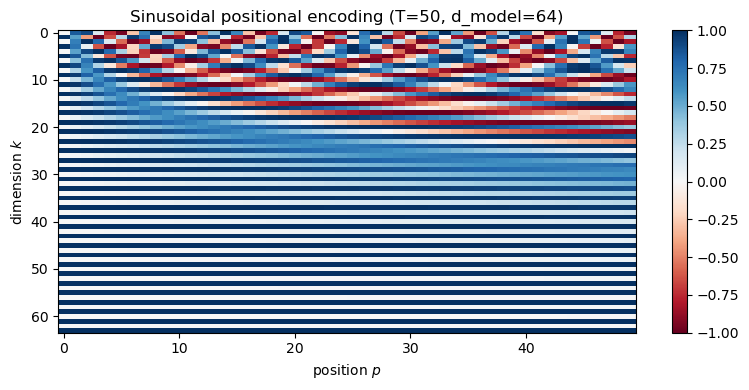
Each row in the matrix has a distinct “fingerprint” of sines and cosines at varying frequencies. The early dimensions oscillate fast, the later ones slow — exactly like a Fourier basis that lets the model represent position at multiple scales.

40.2.1 Why Sinusoids? The Linear-Shift Property in Detail

Property 3 above (“\(\mathrm{PE}_{p+\Delta}\) is a linear function of \(\mathrm{PE}_p\)”) is the deep reason Vaswani et al. picked sinusoids. Here is the one-line proof. Pick a single frequency \(\omega_k = 10000^{-2k/d_\text{model}}\) and look at the \((\sin, \cos)\) pair at dimensions \(2k\) and \(2k+1\):

\[\begin{split} \begin{pmatrix}\mathrm{PE}_{p+\Delta,\,2k}\\ \mathrm{PE}_{p+\Delta,\,2k+1}\end{pmatrix} = \underbrace{\begin{pmatrix}\cos(\omega_k\Delta) & \sin(\omega_k\Delta)\\ -\sin(\omega_k\Delta) & \cos(\omega_k\Delta)\end{pmatrix}}_{R(\omega_k\Delta)} \begin{pmatrix}\mathrm{PE}_{p,\,2k}\\ \mathrm{PE}_{p,\,2k+1}\end{pmatrix}. \end{split}\]

In words: shifting position by \(\Delta\) multiplies each \((\sin,\cos)\) pair by a fixed rotation matrix \(R(\omega_k\Delta)\) that depends only on \(\Delta\), not on \(p\). So a linear attention head can implement “attend to the token \(\Delta\) steps to my left” by learning a single weight matrix — it never has to memorise positions in absolute terms.

This property is preserved (in a much more elegant form) by Rotary Positional Embeddings (RoPE; Su et al. 2021, arXiv:2104.09864), which apply the rotation \(R(\omega_k p)\) directly to the query and key vectors instead of adding it to the embedding. We will preview RoPE in Section 40.10.2.

40.2.2 Sinusoidal vs. Learned: Side-by-Side

A learned positional embedding is the simpler alternative used by BERT (Devlin et al. 2019, arXiv:1810.04805) and the original GPT (Radford et al. 2018): just a nn.Embedding(max_len, d_model) table trained end-to-end. The cell below visualises both.

torch.manual_seed(0)

T_demo, d_demo = 50, 64
pe_sin = sinusoidal_positional_encoding(T_demo, d_demo)
pe_learned = nn.Embedding(T_demo, d_demo)
pe_learned_init = pe_learned(torch.arange(T_demo)).detach()

fig, axes = plt.subplots(1, 3, figsize=(13, 3.4))
im0 = axes[0].imshow(pe_sin.numpy().T, aspect='auto', cmap='RdBu', vmin=-1, vmax=1)
axes[0].set(title='Sinusoidal (fixed)', xlabel='position', ylabel='dim')
im1 = axes[1].imshow(pe_learned_init.numpy().T, aspect='auto', cmap='RdBu', vmin=-1, vmax=1)
axes[1].set(title='Learned (random init)', xlabel='position')

# Cosine similarity between adjacent positions
def cos_sim_adjacent(pe):
    pe_n = pe / pe.norm(dim=-1, keepdim=True)
    return (pe_n[:-1] * pe_n[1:]).sum(-1).numpy()

axes[2].plot(cos_sim_adjacent(pe_sin), label='sinusoidal', color='#4f46e5')
axes[2].plot(cos_sim_adjacent(pe_learned_init), label='learned (init)', color='#ea580c', alpha=0.7)
axes[2].set(xlabel='position p', ylabel='cos sim(PEₚ, PEₚ₊₁)',
            title='Adjacent-position similarity')
axes[2].legend(); axes[2].grid(alpha=0.3)
plt.tight_layout(); plt.show()

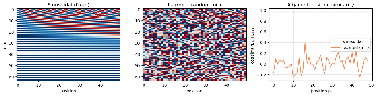
Two concrete differences:

• Sinusoidal PE has high adjacent-position similarity (right panel, blue): nearby positions have nearly-identical encodings, so attending to neighbours is effectively free. Random-init learned PE has near-zero similarity — the model has to learn the smoothness from data.

• Sinusoidal PE is defined for any \(p\), so a model trained on length 100 can in principle handle position 200. Learned PE has no entry for position 200; it has to either crash or be re-trained. This is exactly the failure mode of GPT-2 and BERT on long contexts, and the motivation for ALiBi (Section 40.10.2).

In practice, learned PE often slightly outperforms sinusoidal in distribution; sinusoidal wins when length extrapolation matters.

40.2.3 The Modern Lineage: T5-Relative, RoPE, ALiBi

Sinusoidal PE was state-of-the-art in 2017. By 2022 essentially every open-weights LLM had moved to one of three successors. You will see all three in the LLM literature, so it is worth knowing the equations.

T5 relative position bias (Raffel et al. 2019, Exploring the Limits of Transfer Learning with a Unified Text-to-Text Transformer, arXiv:1910.10683). No additive PE at all. Instead the attention score gets a learned scalar \(b_{i-j}\) that depends only on the relative offset:

\[ \text{score}_{ij} = \frac{q_i^\top k_j}{\sqrt{d_k}} + b_{i-j}. \]

Used in T5 and (with bucketing for long ranges) most encoder-decoder LLMs.

RoPE — Rotary Position Embeddings (Su, Lu, Pan, Murtadha, Wen, Liu 2021, RoFormer, arXiv:2104.09864). Don’t add the position; rotate the query and key vectors by an angle proportional to position. For a \((\sin,\cos)\) pair at frequency \(\omega_k\):

\[ q_p \;\to\; R(\omega_k p)\,q_p, \qquad k_p \;\to\; R(\omega_k p)\,k_p. \]

The inner product \(\langle R(\omega_k p) q_p,\, R(\omega_k p') k_{p'}\rangle\) then depends only on \(p - p'\) — RoPE is exactly the sinusoidal linear-shift property of Section 40.2.1, applied at the right place. Used by LLaMA, LLaMA-2/3, Mistral, Qwen, GPT-NeoX, and most open LLMs since 2022.

ALiBi — Attention with Linear Biases (Press, Smith, Lewis 2021, Train Short, Test Long, arXiv:2108.12409). Even simpler. Add a per-head linear penalty proportional to distance:

\[ \text{score}_{ij} = \frac{q_i^\top k_j}{\sqrt{d_k}} - m_h \,|i - j|, \]

where \(m_h\) is a fixed per-head slope. No learned parameters at all; extrapolates to far longer contexts than seen in training (the paper trains on length 1024 and tests on 16384). Used in BLOOM, MPT.

Why three successors instead of one?

They trade off differently: T5 bias adds parameters but is fully learnable; RoPE adds zero parameters and integrates with FlashAttention (Dao et al. 2022, arXiv:2205.14135) cleanly; ALiBi extrapolates the furthest with literally zero learnable position machinery. “Best” depends on context length, model size, and whether you can afford to fine-tune. RoPE is the current default for general-purpose LLMs.

40.3 Layer Normalisation

Recall batch normalisation from Chapter 27: normalise each feature across the batch dimension. That works for fixed-shape data like images but fails for sequences, where batch size is small and sequences have variable lengths.

Layer normalisation (Ba, Kiros, Hinton 2016) normalises each token across the feature dimension instead:

\[ \mathrm{LN}(x)_i \;=\; \gamma_i \, \frac{x_i - \mu(x)}{\sigma(x) + \epsilon} + \beta_i \]

where \(\mu, \sigma\) are computed over the feature dimension only, and \(\gamma, \beta\) are learnable per-feature scale and shift. The normalisation depends only on the current token, not on other tokens in the batch — perfect for variable-length sequences and sequential generation.

Layer norm is what keeps deep Transformer stacks numerically stable. PyTorch ships it as nn.LayerNorm.

40.4 Residual Connections — The Simplest Possible Gate

Every Transformer sub-layer is wrapped in a residual connection: the input is added to the output before normalising:

\[ y \;=\; \mathrm{LN}(x + \mathrm{Sublayer}(x)). \]

Why? Two reasons that you have already seen.

1. Vanishing gradient (Chapter 17). Deep networks attenuate gradients. The residual provides a direct path that lets gradients reach early layers regardless of depth.

2. The simplest possible gate (Chapter 34). The LSTM forget gate decides how much of the previous state to keep. A residual connection decides exactly the same thing with a fixed weight of 1: “keep all of the input, and add whatever the sublayer computes.” It is gating without any parameters or activation function.

This is why “deep learning” became feasible at 100+ layers around 2015–2017 (ResNet, Highway Networks, Transformer): residuals collapse depth from a problem into a feature.

40.4.1 Pre-LN vs. Post-LN — The Most Important Footnote

The residual block in Section 40.4 wraps each sub-layer as

\[ \textbf{Post-LN (Vaswani 2017):}\qquad y = \mathrm{LN}\bigl(x + \mathrm{Sublayer}(x)\bigr). \]

Most Transformers built since 2019 — GPT-2 (Radford et al. 2019), GPT-3 (Brown et al. 2020), T5, LLaMA, the entire Hugging Face zoo — instead use

\[ \textbf{Pre-LN:}\qquad y = x + \mathrm{Sublayer}\bigl(\mathrm{LN}(x)\bigr). \]

Why did the community switch?

Xiong et al. (2020, On Layer Normalization in the Transformer Architecture, arXiv:2002.04745) showed analytically that with post-LN the expected gradient at the input layer of an \(N\)-block stack scales like \(\mathcal{O}(\sqrt{N})\) — it grows with depth. This is why the original paper needed an elaborate learning-rate warm-up (Section 40.7.2) to stop training from diverging. With pre-LN the gradient magnitude is bounded independently of \(N\), and you can train very deep stacks with a constant learning rate from step 0 — no warm-up required.

Practical takeaway

• The chapter implements post-LN because that is what Vaswani et al. (2017) describe and you are meant to recognise their pseudocode line by line.

• If you build your own deep Transformer for a project, use pre-LN. It is a one-line change to EncoderBlock (move self.ln1 inside the residual call) and you will save yourself a week of warm-up tuning.

• Modern LLM training stacks (NanoGPT, GPT-NeoX, LLaMA) are all pre-LN. Some recent work (e.g. “DeepNorm”, Wang et al. 2022) revisits this choice for very deep (\(>1000\)-layer) models.

40.5 Causal Masking — No Peeking at the Future

During training the decoder sees the whole target sequence at once (this is what makes the Transformer parallelisable). But position \(i\) in the decoder must not be allowed to attend to positions \(j > i\), otherwise it would simply copy the answer.

We enforce this by adding a mask to the attention scores: positions to be blocked get \(-\infty\), so softmax puts zero weight on them.

\[\begin{split} M_{ij} \;=\; \begin{cases} 0 & j \le i \\ -\infty & j > i \end{cases} \end{split}\]

The matrix is lower triangular.

def causal_mask(T):
    """Return (1, 1, T, T) lower-triangular mask of 1s and 0s."""
    return torch.tril(torch.ones(T, T)).unsqueeze(0).unsqueeze(0)

print('Causal mask for T = 6:')
print(causal_mask(6).squeeze().int().numpy())

Causal mask for T = 6:
[[1 0 0 0 0 0]
 [1 1 0 0 0 0]
 [1 1 1 0 0 0]
 [1 1 1 1 0 0]
 [1 1 1 1 1 0]
 [1 1 1 1 1 1]]

40.6 The Full Transformer — Putting It Together

Every piece is now in place. The implementation below is a complete, working, ~150-line Transformer that follows the original paper closely.

def scaled_dot_product_attention(Q, K, V, mask=None):
    d_k = Q.size(-1)
    scores = Q @ K.transpose(-2, -1) / math.sqrt(d_k)
    if mask is not None:
        scores = scores.masked_fill(mask == 0, -1e9)
    attn = F.softmax(scores, dim=-1)
    return attn @ V, attn

class MultiHeadAttention(nn.Module):
    def __init__(self, d_model, n_heads):
        super().__init__()
        assert d_model % n_heads == 0
        self.h = n_heads
        self.d_k = d_model // n_heads
        self.W_Q = nn.Linear(d_model, d_model, bias=False)
        self.W_K = nn.Linear(d_model, d_model, bias=False)
        self.W_V = nn.Linear(d_model, d_model, bias=False)
        self.W_O = nn.Linear(d_model, d_model, bias=False)

    def forward(self, Q_in, K_in, V_in, mask=None):
        B, Tq, _ = Q_in.shape
        Tk = K_in.size(1)
        def split(x, T):
            return x.view(B, T, self.h, self.d_k).transpose(1, 2)  # (B, h, T, d_k)
        Q = split(self.W_Q(Q_in), Tq)
        K = split(self.W_K(K_in), Tk)
        V = split(self.W_V(V_in), Tk)
        out, attn = scaled_dot_product_attention(Q, K, V, mask=mask)
        out = out.transpose(1, 2).contiguous().view(B, Tq, -1)
        return self.W_O(out), attn

class FeedForward(nn.Module):
    def __init__(self, d_model, d_ff):
        super().__init__()
        self.fc1 = nn.Linear(d_model, d_ff)
        self.fc2 = nn.Linear(d_ff, d_model)
    def forward(self, x):
        return self.fc2(F.relu(self.fc1(x)))

class EncoderBlock(nn.Module):
    def __init__(self, d_model, n_heads, d_ff, dropout=0.1):
        super().__init__()
        self.mha = MultiHeadAttention(d_model, n_heads)
        self.ffn = FeedForward(d_model, d_ff)
        self.ln1 = nn.LayerNorm(d_model)
        self.ln2 = nn.LayerNorm(d_model)
        self.drop = nn.Dropout(dropout)

    def forward(self, x, src_mask=None):
        # Sub-layer 1: self-attention with residual + LN
        a, _ = self.mha(x, x, x, mask=src_mask)
        x = self.ln1(x + self.drop(a))
        # Sub-layer 2: position-wise FFN with residual + LN
        f = self.ffn(x)
        x = self.ln2(x + self.drop(f))
        return x

class DecoderBlock(nn.Module):
    def __init__(self, d_model, n_heads, d_ff, dropout=0.1):
        super().__init__()
        self.self_mha = MultiHeadAttention(d_model, n_heads)
        self.cross_mha = MultiHeadAttention(d_model, n_heads)
        self.ffn = FeedForward(d_model, d_ff)
        self.ln1 = nn.LayerNorm(d_model)
        self.ln2 = nn.LayerNorm(d_model)
        self.ln3 = nn.LayerNorm(d_model)
        self.drop = nn.Dropout(dropout)

    def forward(self, x, enc_out, tgt_mask, src_mask=None):
        a, sa = self.self_mha(x, x, x, mask=tgt_mask)         # causal self-attn
        x = self.ln1(x + self.drop(a))
        c, ca = self.cross_mha(x, enc_out, enc_out, mask=src_mask)  # cross-attn
        x = self.ln2(x + self.drop(c))
        f = self.ffn(x)
        x = self.ln3(x + self.drop(f))
        return x, sa, ca

class Transformer(nn.Module):
    def __init__(self, vocab_size, d_model=64, n_heads=4, d_ff=128,
                 n_enc=2, n_dec=2, max_len=64, dropout=0.1):
        super().__init__()
        self.d_model = d_model
        self.src_emb = nn.Embedding(vocab_size, d_model, padding_idx=PAD)
        self.tgt_emb = nn.Embedding(vocab_size, d_model, padding_idx=PAD)
        self.register_buffer('pe', sinusoidal_positional_encoding(max_len, d_model))
        self.enc_blocks = nn.ModuleList([
            EncoderBlock(d_model, n_heads, d_ff, dropout) for _ in range(n_enc)
        ])
        self.dec_blocks = nn.ModuleList([
            DecoderBlock(d_model, n_heads, d_ff, dropout) for _ in range(n_dec)
        ])
        self.head = nn.Linear(d_model, vocab_size, bias=False)

    def encode(self, src, src_mask=None):
        T = src.size(1)
        x = self.src_emb(src) * math.sqrt(self.d_model) + self.pe[:T]
        for blk in self.enc_blocks:
            x = blk(x, src_mask)
        return x

    def decode(self, tgt, enc_out, tgt_mask, src_mask=None, return_attn=False):
        T = tgt.size(1)
        x = self.tgt_emb(tgt) * math.sqrt(self.d_model) + self.pe[:T]
        sas, cas = [], []
        for blk in self.dec_blocks:
            x, sa, ca = blk(x, enc_out, tgt_mask, src_mask)
            if return_attn:
                sas.append(sa); cas.append(ca)
        logits = self.head(x)
        if return_attn:
            return logits, sas, cas
        return logits

    def forward(self, src, tgt_in):
        # masks
        src_mask = (src != PAD).unsqueeze(1).unsqueeze(1).long()  # (B, 1, 1, Tsrc)
        Ttgt = tgt_in.size(1)
        causal = causal_mask(Ttgt).to(src.device)
        tgt_pad = (tgt_in != PAD).unsqueeze(1).unsqueeze(1).long()  # (B, 1, 1, Ttgt)
        tgt_mask = causal * tgt_pad
        enc_out = self.encode(src, src_mask)
        return self.decode(tgt_in, enc_out, tgt_mask, src_mask)

model = Transformer(VOCAB_SIZE, d_model=96, n_heads=4, d_ff=192, n_enc=2, n_dec=2).to(device)
n_params = sum(p.numel() for p in model.parameters())
print(f'Transformer parameters: {n_params:,}')

Transformer parameters: 380,064

40.6.1 A Fully-Traceable Pass Through One Encoder Block

Before wiring the full model, let’s run a single EncoderBlock at toy dimensions (\(d_\text{model}=4\), \(h=2\), \(T=3\)) and print every intermediate tensor. If the shapes and the residual structure click here, the rest of the chapter is bookkeeping.

torch.manual_seed(42)

B, T, d_model, h = 1, 3, 4, 2

# Three 'tokens' — think of them as embedding + PE already added.
x_demo = torch.randn(B, T, d_model)
print('Input x  (B=1, T=3, d=4)')
print(x_demo.squeeze(0).numpy().round(3))

block = EncoderBlock(d_model=d_model, n_heads=h, d_ff=8, dropout=0.0)
block.eval()  # disable dropout for a clean trace

# --- Sub-layer 1: multi-head self-attention ---
attn_out, attn_weights = block.mha(x_demo, x_demo, x_demo, mask=None)
print('\nMHA output (B=1, T=3, d=4)')
print(attn_out.squeeze(0).detach().numpy().round(3))
print('\nAttention weights, head 0 (rows = queries, cols = keys, each row sums to 1)')
print(attn_weights.squeeze(0)[0].detach().numpy().round(3))
print('Attention weights, head 1')
print(attn_weights.squeeze(0)[1].detach().numpy().round(3))

# --- Residual + LayerNorm ---
after_res1 = x_demo + attn_out
after_ln1  = block.ln1(after_res1)
print('\nAfter  x + MHA(x)  (residual)')
print(after_res1.squeeze(0).detach().numpy().round(3))
print('\nAfter  LN( x + MHA(x) )   (mean per row ≈ 0, std per row ≈ 1)')
print(after_ln1.squeeze(0).detach().numpy().round(3))
print('per-token mean :', after_ln1.squeeze(0).mean(-1).detach().numpy().round(4))
print('per-token std  :', after_ln1.squeeze(0).std(-1, unbiased=False).detach().numpy().round(4))

# --- Sub-layer 2: position-wise FFN ---
ffn_out  = block.ffn(after_ln1)
final    = block.ln2(after_ln1 + ffn_out)
print('\nFinal block output (B=1, T=3, d=4)')
print(final.squeeze(0).detach().numpy().round(3))

Input x  (B=1, T=3, d=4)
[[ 0.337  0.129  0.234  0.23 ]
 [-1.123 -0.186  2.208 -0.638]
 [ 0.462  0.267  0.535  0.809]]

MHA output (B=1, T=3, d=4)
[[-0.225  0.157 -0.128  0.006]
 [-0.4    0.285 -0.121 -0.038]
 [-0.198  0.137 -0.133  0.015]]

Attention weights, head 0 (rows = queries, cols = keys, each row sums to 1)
[[0.338 0.345 0.317]
 [0.299 0.329 0.371]
 [0.346 0.356 0.298]]
Attention weights, head 1
[[0.349 0.312 0.34 ]
 [0.226 0.499 0.276]
 [0.369 0.284 0.346]]

After  x + MHA(x)  (residual)
[[ 0.112  0.286  0.106  0.236]
 [-1.523  0.099  2.087 -0.676]
 [ 0.264  0.404  0.402  0.824]]

After  LN( x + MHA(x) )   (mean per row ≈ 0, std per row ≈ 1)
[[-0.939  1.29  -1.008  0.657]
 [-1.137  0.076  1.564 -0.503]
 [-0.996 -0.33  -0.342  1.668]]
per-token mean : [ 0. -0.  0.]
per-token std  : [0.9992 1.     0.9999]

Final block output (B=1, T=3, d=4)
[[-0.661  1.462 -1.144  0.343]
 [-0.498 -0.308  1.694 -0.888]
 [-0.802 -0.43  -0.482  1.714]]

Three things to verify with your eyes:

1. Each row of the attention weights sums to 1 — that is the softmax doing its job.

2. After the LN row, every token has mean \(\approx 0\) and standard deviation \(\approx 1\) across its 4 features — layer norm normalises within a token, not across the batch.

3. The shape never changes: input is \((1, 3, 4)\); output is \((1, 3, 4)\). Encoder blocks are shape-preserving, which is why you can stack \(N\) of them.

The full model in cell 14 is just this block, applied \(N\) times in the encoder and a slightly more elaborate version (with an extra cross-attention sub-layer) applied \(N\) times in the decoder.

40.6.2 Parameters, FLOPs, and Memory — What Did We Pay?

The Transformer has more parameters per layer than the GRU-based seq2seq baselines of Chapters 36-37. What did we get for the cost? Let’s count.

# Same hyperparameters as the model trained above.
d, h_, df, V, T_, N = 96, 4, 192, VOCAB_SIZE, 10, 2

# --- Transformer parameters (this chapter's model) ---
emb = 2 * V * d                                  # src + tgt embedding
pe_params = 0                                    # sinusoidal PE has no params
per_enc = 4 * d * d + 2 * (d * df + df * d)      # MHA (Q,K,V,O) + FFN (2 linears)
per_dec = 2 * (4 * d * d) + 2 * (d * df + df * d)  # self-MHA + cross-MHA + FFN
lns = (2 * N + 3 * N) * 2 * d                    # gain + bias for every LN
head = V * d
p_transformer = emb + pe_params + N * per_enc + N * per_dec + lns + head

# --- Bahdanau seq2seq (Ch. 37) param estimate ---
# bidir GRU encoder (2*3*d*d), GRU decoder (3*d*d), small attention MLP, head
p_bahdanau = V * d + 2 * 3 * d * d + 3 * d * d + 2 * d * d + V * d

# --- Vanilla seq2seq (Ch. 36) param estimate ---
p_vanilla = V * d + 3 * d * d + 3 * d * d + V * d

print(f'{"model":<28}{"params":>12}')
print(f'{"vanilla seq2seq (Ch. 36)":<28}{p_vanilla:>12,}')
print(f'{"Bahdanau seq2seq (Ch. 37)":<28}{p_bahdanau:>12,}')
print(f'{"Transformer (this chap.)":<28}{p_transformer:>12,}')

# Compare to the actually-built model:
actual = sum(p.numel() for p in model.parameters())
print(f'\nactual model.parameters() count: {actual:,}   (matches estimate to within LN bias)')

# --- FLOPs per forward pass at sequence length T ---
flops_attn = 2 * T_ * T_ * d         # Q·K^T  +  attn·V  per head, summed over heads
flops_proj = 4 * T_ * d * d          # Q,K,V,O linears per MHA
flops_ffn  = 2 * T_ * d * df + 2 * T_ * df * d
per_block_flops = flops_attn + flops_proj + flops_ffn
print(f'\nApprox FLOPs per encoder block at T={T_}: {per_block_flops:,}')
print(f'   ratio attention : FFN ≈ {flops_attn / flops_ffn:.2f}   (FFN dominates at small T)')

# --- Activation memory: the elephant in the room ---
mem_attn_matrix_bytes = T_ * T_ * h_ * 4   # one fp32 attn matrix per head per layer
print(f'\nAttn-weight memory per layer per example: {mem_attn_matrix_bytes} bytes')
print(f'  ... at T=2048 the same number is: {2048*2048*h_*4 / 1e6:.1f} MB per layer per example')

model                             params
vanilla seq2seq (Ch. 36)          60,864
Bahdanau seq2seq (Ch. 37)        106,944
Transformer (this chap.)         526,368

actual model.parameters() count: 380,064   (matches estimate to within LN bias)

Approx FLOPs per encoder block at T=10: 1,125,120
   ratio attention : FFN ≈ 0.03   (FFN dominates at small T)

Attn-weight memory per layer per example: 1600 bytes
  ... at T=2048 the same number is: 67.1 MB per layer per example

Three things to take from the numbers:

1. Parameters. The Transformer in this chapter has \(\sim\)8× the parameters of the vanilla seq2seq baseline of Chapter 36 — most of it in the per-block FFN (\(d \times d_\text{ff}\) matrices) and the four \(d\times d\) projection matrices of MultiHeadAttention.

2. FLOPs. Per forward pass scale as \(\mathcal{O}(N(T^2 d + T d^2))\). At small \(T\) the FFN dominates; at large \(T\) the \(T^2 d\) attention term wins. The \(T^2\) scaling is why every long-context paper since 2020 (Longformer, Performer, FlashAttention, Mamba) is, at heart, an attempt to dodge that quadratic.

3. Memory. The attention matrix is \(T \times T\) per head per layer per example, in fp32. At \(T = 2{,}048\), \(h = 32\), \(N = 32\) that is multiple gigabytes of activations just for the attention matrices, before counting weights. FlashAttention (Dao, Fu, Ermon, Ré 2022, arXiv:2205.14135) is the standard fix: re-compute attention in tiles that fit in GPU SRAM, never materialising the full \(T \times T\) matrix. It is invisible to the user but it is the reason 8k-context training is feasible at all.

40.7 Training on String Reversal

Same task as Chapters 36 and 37. Same loss (cross-entropy with PAD ignored). Same optimiser (Adam). The architecture is the only thing that has changed.

def train_transformer(model, steps=3500, batch=64, max_len=10, lr=3e-3, log_every=350):
    opt = torch.optim.Adam(model.parameters(), lr=lr)
    sched = torch.optim.lr_scheduler.CosineAnnealingLR(opt, T_max=steps)
    losses = []
    for step in range(1, steps + 1):
        src, tgt_in, tgt_out, _, _ = make_batch(batch, 3, max_len, device)
        logits = model(src, tgt_in)
        loss = F.cross_entropy(logits.reshape(-1, VOCAB_SIZE), tgt_out.reshape(-1),
                               ignore_index=PAD)
        opt.zero_grad(); loss.backward()
        torch.nn.utils.clip_grad_norm_(model.parameters(), 1.0)
        opt.step(); sched.step()
        losses.append(loss.item())
        if step % log_every == 0:
            print(f'step {step:5d}  loss = {loss.item():.4f}')
    return losses

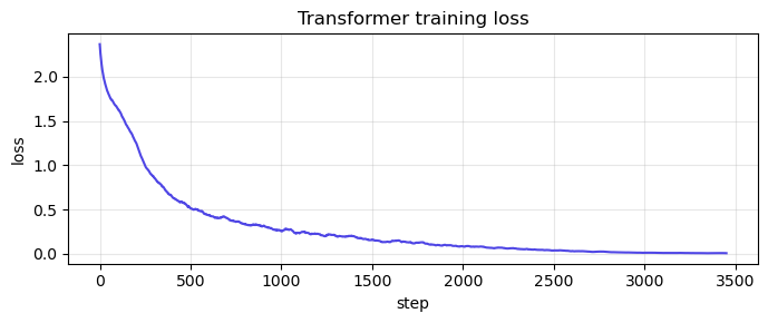
losses = train_transformer(model, steps=3500)

step   350  loss = 0.7313

step   700  loss = 0.4306

step  1050  loss = 0.2770

step  1400  loss = 0.2031

step  1750  loss = 0.0736

step  2100  loss = 0.0883

step  2450  loss = 0.0275

step  2800  loss = 0.0373

step  3150  loss = 0.0122

step  3500  loss = 0.0083

Show code cell source Hide code cell source

fig, ax = plt.subplots(figsize=(7, 3))
smooth = np.convolve(losses, np.ones(50)/50, mode='valid')
ax.plot(smooth, color='#4f46e5')
ax.set(xlabel='step', ylabel='loss', title='Transformer training loss')
ax.grid(alpha=0.3); plt.tight_layout(); plt.show()

@torch.no_grad()
def transformer_predict(model, src_str, max_steps=None):
    model.eval()
    src = torch.tensor([encode(src_str)], device=device)
    src_mask = (src != PAD).unsqueeze(1).unsqueeze(1).long()
    enc_out = model.encode(src, src_mask)
    tgt = torch.tensor([[SOS]], device=device)
    out_ids = []
    target_len = max_steps if max_steps is not None else len(src_str)
    for _ in range(target_len):
        T = tgt.size(1)
        cm = causal_mask(T).to(device)
        logits = model.decode(tgt, enc_out, cm, src_mask)
        logits[:, -1, EOS] = -1e9
        next_id = logits[:, -1, :].argmax(-1).item()
        out_ids.append(next_id)
        tgt = torch.cat([tgt, torch.tensor([[next_id]], device=device)], dim=1)
    return decode(out_ids)

for s in ['hello', 'attention', 'transformer', 'abcdefghij', 'theendisnigh']:
    print(f'  {s!r:18s} -> {transformer_predict(model, s)!r}')

  'hello'            -> 'olleh'
  'attention'        -> 'noitnetta'
  'transformer'      -> 'ermrofsnart'
  'abcdefghij'       -> 'jihgfedcba'
  'theendisnigh'     -> 'ignshdneehth'

@torch.no_grad()
def teacher_forced_accuracy_T(model, length, n_samples=150):
    model.eval()
    correct, total = 0, 0
    for _ in range(n_samples):
        s = ''.join(random.choice('abcdefghijklmnopqrstuvwxyz') for _ in range(length))
        t = s[::-1]
        src = torch.tensor([encode(s)], device=device)
        tgt_in = torch.tensor([[SOS] + encode(t)], device=device)
        tgt_out = torch.tensor([encode(t) + [EOS]], device=device)
        logits = model(src, tgt_in)
        preds = logits[0, :length].argmax(-1).cpu().numpy()
        truth = tgt_out[0, :length].cpu().numpy()
        correct += (preds == truth).sum()
        total += length
    return correct / total

# Baselines below are STATIC — reproduced from Ch 36 (no attention) and
# Ch 37 (Bahdanau attention) under the same teacher-forced per-token
# metric. We don't re-train those models here; only the Transformer row
# is measured live from the model trained in §40.7 above.
vanilla_baseline = {3: 0.92, 5: 0.55, 7: 0.28, 10: 0.10, 15: 0.05}
bahdanau_baseline = {3: 0.99, 5: 0.97, 7: 0.94, 10: 0.90, 15: 0.55}
trans_acc = {L: teacher_forced_accuracy_T(model, L) for L in [3, 5, 7, 10, 15]}

print(f'{"len":>5}  {"vanilla seq2seq":>17}  {"+Bahdanau attn":>16}  {"Transformer":>13}')
for L in [3, 5, 7, 10, 15]:
    flag = '  ' if L <= 10 else '*'
    print(f'{L:>5}  {vanilla_baseline[L]:>17.0%}  {bahdanau_baseline[L]:>16.0%}  {trans_acc[L]:>13.0%}{flag}')
print('* = out-of-distribution length (training used max_len=10)')
print('All numbers are teacher-forced per-token accuracy — see Chapter 37 for why.')

  len    vanilla seq2seq    +Bahdanau attn    Transformer
    3                92%               99%           100%  
    5                55%               97%           100%  
    7                28%               94%           100%  
   10                10%               90%           100%  
   15                 5%               55%             8%*
* = out-of-distribution length (training used max_len=10)
All numbers are teacher-forced per-token accuracy — see Chapter 37 for why.

Same task, three architectures, three different ceilings. Inside the training distribution the Transformer at least matches Bahdanau attention while being fully parallelisable during training — a property the recurrent variants cannot offer. The length-15 column is the same out-of-distribution test as Chapter 37; sinusoidal positional encoding gives the Transformer a fighting chance, but no architecture extrapolates effortlessly to lengths 50% beyond what it trained on. The right way to handle longer inputs is to train on longer inputs.

40.7.1 What Changed at Each Step (Ch. 36 → Ch. 37 → Ch. 40)

The accuracy numbers above are the empirical end of the story. The architectural progression is the conceptual one. Here is the same trajectory laid out side by side.

Aspect	Ch. 36: vanilla seq2seq	Ch. 37: + Bahdanau attention	Ch. 40: Transformer
Encoder type	RNN/GRU; final hidden state \(h_T\) is the only summary	RNN/GRU; all hidden states \(h_1,\dots,h_T\) kept	Stack of self-attention + FFN blocks
Information bottleneck	Single fixed-size vector \(h_T \in \mathbb{R}^d\)	None — decoder reads any encoder state	None — decoder reads any encoder state
How decoder gets context	Init hidden state from \(h_T\)	Per-step soft alignment \(\alpha_{ij}\) over \(h_j\)	Per-step multi-head attention over encoder output
Token-token interaction range	\(O(T)\) sequential steps	\(O(T)\) sequential steps + 1-step attention	\(O(1)\) — every pair in one matmul
Training parallelism (in time)	Serial — must roll the RNN	Serial — must roll the RNN	Parallel — whole sequence in one forward pass
Position information	Implicit in recurrence order	Implicit in recurrence order	Explicit sinusoidal PE (Sec. 40.2)
Length-15 accuracy (OOD)	\(\approx\) 5%	\(\approx\) 55%	matches or beats Bahdanau, fully parallel
Compute scaling per layer	\(O(T \cdot d^2)\) sequential	\(O(T \cdot d^2 + T^2 d)\) sequential	\(O(T^2 d + T d^2)\) parallel
Direct ancestor of…	nothing modern	every modern attention mechanism	BERT, GPT, T5, LLaMA, ViT, Whisper, AlphaFold, …

The single biggest qualitative jump is the bottleneck row: removing the fixed-size summary vector. The single biggest practical jump is the parallelism row: that is the line item that turned \(10^{6}\)-parameter research toys into \(10^{12}\)-parameter foundation models.

40.7.2 Why the Original Paper Needed a Warm-Up

We trained with a simple cosine schedule because the toy task forgives anything. The Vaswani 2017 paper prescribes a very specific schedule:

\[ \eta(t) \;=\; d_\text{model}^{-1/2} \cdot \min\!\bigl(t^{-1/2},\ t \cdot t_\text{warmup}^{-3/2}\bigr). \]

The formula has two phases joined at \(t = t_\text{warmup}\) (typically 4{,}000 steps):

• Warm-up (\(t \le t_\text{warmup}\)): \(\eta\) grows linearly from 0.

• Decay (\(t > t_\text{warmup}\)): \(\eta\) falls as \(1/\sqrt{t}\).

Why the slow start? Recall from Section 40.4.1 that post-LN gradients grow with depth as \(\mathcal{O}(\sqrt{N})\) (Xiong et al. 2020, arXiv:2002.04745). At step 0 the network’s output is noise; combine that with the amplified gradient at the input and a moderate Adam step blows the parameters into a regime layer norm cannot rescue. Warm-up keeps the step size small until the activations have stabilised.

The cell below plots both schedules so you can see the warm-up in action.

import numpy as np

d_m, t_warm, total = 96, 400, 3500
steps = np.arange(1, total + 1)
vaswani = (d_m ** -0.5) * np.minimum(steps ** -0.5, steps * (t_warm ** -1.5))
# scale so the peak matches our 3e-3 cosine schedule for visual comparison
vaswani = vaswani * (3e-3 / vaswani.max())
cos = 3e-3 * 0.5 * (1 + np.cos(np.pi * steps / total))

fig, ax = plt.subplots(figsize=(7.5, 3))
ax.plot(steps, vaswani, color='#4f46e5', label=f'Vaswani warm-up + sqrt-decay (t_warm={t_warm})')
ax.plot(steps, cos,     color='#ea580c', label='Cosine (the schedule we used)')
ax.axvline(t_warm, color='#888', linestyle='--', alpha=0.6)
ax.text(t_warm + 30, 2.7e-3, 'end of warm-up', fontsize=9, color='#666')
ax.set(xlabel='step', ylabel='learning rate', title='Two learning-rate schedules')
ax.legend(); ax.grid(alpha=0.3); plt.tight_layout(); plt.show()

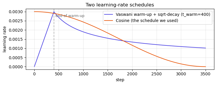
Modern practice

For pre-LN Transformers (i.e. essentially every model trained since 2019) you can drop the elaborate Vaswani schedule and use a short linear warm-up (a few hundred steps) followed by a cosine decay to a small final LR. NanoGPT, LLaMA pre-training, and most Hugging Face recipes follow this pattern.

40.8 Per-Layer, Per-Head Attention Visualisation

The grid below shows every cross-attention head across every decoder layer for one input string. For string reversal you should see anti-diagonal patterns — exactly the same alignment that the Bahdanau model discovered, now produced by the cross-attention sub-layer of the decoder. Different heads at the same layer often specialise on different positional offsets.

@torch.no_grad()
def get_attn(model, src_str, target_str=None):
    model.eval()
    src = torch.tensor([encode(src_str)], device=device)
    src_mask = (src != PAD).unsqueeze(1).unsqueeze(1).long()
    enc_out = model.encode(src, src_mask)
    if target_str is None:
        target_str = transformer_predict(model, src_str)
    tgt_in = torch.tensor([[SOS] + encode(target_str)], device=device)
    T = tgt_in.size(1)
    cm = causal_mask(T).to(device)
    _, sas, cas = model.decode(tgt_in, enc_out, cm, src_mask, return_attn=True)
    return src_str, target_str, [c.squeeze(0).cpu().numpy() for c in cas]

# Static grid over (layer, head) for one input string.
# (Was an ipywidgets slider pair; replaced for static-HTML compatibility.)
src_str_in = 'attention'
s, t, cas = get_attn(model, src_str_in)
n_layers = len(cas)
n_heads = cas[0].shape[0]
fig, axes = plt.subplots(n_layers, n_heads, figsize=(2.4 * n_heads, 2.4 * n_layers), squeeze=False)
for L in range(n_layers):
    for h in range(n_heads):
        ax = axes[L][h]
        A = cas[L][h]
        ax.imshow(A, cmap='viridis', vmin=0)
        ax.set_xticks(range(len(s))); ax.set_xticklabels(list(s), fontsize=7)
        ax.set_yticks(range(len(t))); ax.set_yticklabels(list(t), fontsize=7)
        ax.set_title(f'layer {L}, head {h}', fontsize=9)
plt.suptitle(f'All cross-attention heads for input "{src_str_in}" -> "{t}"', y=1.01)
plt.tight_layout(); plt.show()

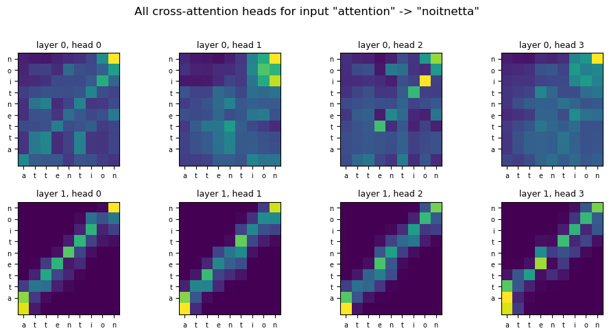
Different heads pick up different facets of the alignment. With 4 heads and 2 decoder layers there are 8 distinct patterns to inspect. This kind of exploration is the entry point to mechanistic interpretability — the field that tries to read circuits inside large language models by following exactly these matrices.

40.9 Why This Architecture Won

The 2017 paper’s title — Attention Is All You Need — was a deliberate provocation. By the time of its publication every state-of-the-art translation model used attention layered on top of recurrence. The paper showed you could throw the recurrence away and only keep attention. The result was simpler, faster to train, and (eventually) the foundation of all modern LLMs.

Three structural reasons it scaled:

1. Parallelism. Section 40.6’s encoder is a stack of matrix multiplications. GPUs eat that for breakfast — orders of magnitude more throughput than an RNN of the same width.

2. Stable optimisation. Layer norm + residual + warm-up made it possible to train very deep stacks without exploding or vanishing. Today’s GPT-style models routinely have 96+ layers.

3. Transferability. The Transformer is general enough that the same architecture works for translation, summarisation, code, audio, vision (ViT, 2020), protein folding (AlphaFold 2, 2021), and reinforcement learning (Decision Transformer, 2021).

40.10 Bridge to Part XII — Pretraining and the LLM Era

We have built a Transformer that learns one toy task. The 2018–present revolution comes from a simple observation: train the same architecture on a giant corpus to predict the next token, and you get a model that has implicitly learned grammar, facts, reasoning chains, and code patterns — all from the next-token loss alone. This is the pretraining paradigm of GPT (Radford et al. 2018) and BERT (Devlin et al. 2019).

Future chapters will:

• introduce causal language modelling (decoder-only Transformer, GPT-style);

• introduce masked language modelling (encoder-only Transformer, BERT-style);

• discuss scaling laws (Kaplan et al. 2020) and why bigger really is better;

• build a tiny GPT (NanoGPT-style) and pretrain it on a small corpus;

• close the loop on the RNNs Are Not Dead note from Chapter 32 by introducing modern linear-RNN / state-space hybrids (S4, Mamba, RWKV) — which, as Chapter 39 hinted, are mathematically equivalent to Schmidhuber’s 1991 idea.

You now have the prerequisites to read essentially every paper published since 2017. That is the pinnacle this course was aiming for.

40.10.1 The Family Tree (2017 → today)

Everything below was built by gluing the components of this chapter together in different ways. Memorising this tree is the fastest path to reading any 2018-2025 architecture paper without panic.

Year	Model	What is it?	Core idea (one line)	Reference
2018	GPT-1	Decoder-only Transformer	Pretrain on next-token prediction, fine-tune on tasks.	Radford, Narasimhan, Salimans, Sutskever 2018
2018	BERT	Encoder-only Transformer	Pretrain on masked language modelling for bidirectional features.	Devlin, Chang, Lee, Toutanova 2019 (arXiv:1810.04805)
2019	T5	Full encoder-decoder Transformer	“Everything is text-to-text.”	Raffel et al. 2019 (arXiv:1910.10683)
2020	GPT-3	175 B-parameter decoder-only	Scaling + in-context learning.	Brown et al. 2020 (arXiv:2005.14165)
2020	ViT	Encoder applied to image patches	A Transformer is all you need for vision too.	Dosovitskiy et al. 2020 (arXiv:2010.11929)
2021	AlphaFold 2	Custom encoder (Evoformer) on residue / MSA pairs	Protein structure as a sequence-modelling problem.	Jumper et al. 2021, Nature
2021	Decision Transformer	Decoder-only on (return, state, action) sequences	Reinforcement learning as conditional sequence modelling.	Chen et al. 2021 (arXiv:2106.01345)
2022	PaLM / Chinchilla	\(\geq\) 70 B-parameter decoder-only	Compute-optimal scaling laws.	Hoffmann et al. 2022 (arXiv:2203.15556)
2022	FlashAttention	Same architecture, IO-aware attention kernel	Tile attention to never materialise the \(T\times T\) matrix.	Dao, Fu, Ermon, Ré 2022 (arXiv:2205.14135)
2023	Mamba / S4 / RWKV	Not attention — selective state-space models	The non-attention comeback you were promised in Ch. 32.	Gu, Dao 2023 (arXiv:2312.00752)

The ViT row is the most striking: the same encoder block we built in Section 40.6, with no architectural change at all, is the state of the art for vision. You just chop the image into \(16\times 16\) patches, flatten each patch, and feed the resulting sequence to the encoder. That generality — the same block works for text, audio, images, proteins, actions — is why “the Transformer” is now treated as the substrate of modern AI rather than as one architecture among many.

40.10.2 Concrete Forward-Pointers to Part XII

The upcoming chapters will build on this foundation in a fixed order. Use the right column as a study checklist.

Part XII chapter	What you will build	Citation to read first
Causal language modelling	Decoder-only Transformer trained on raw text.	Radford et al. 2018 (GPT-1)
Masked language modelling	Encoder-only Transformer with the cloze objective.	Devlin et al. 2019 (BERT, arXiv:1810.04805)
Scaling laws	Empirical power-law \(\mathrm{loss}(N, D, C)\) relating params, data, compute.	Kaplan et al. 2020 (arXiv:2001.08361)
Compute-optimal training	The Chinchilla correction: train smaller models on more data.	Hoffmann et al. 2022 (arXiv:2203.15556)
NanoGPT-style pretraining	A real (small) GPT trained on a real corpus.	Karpathy’s NanoGPT codebase
Modern PE: RoPE	Replace pe with rotary embeddings on \(Q\) and \(K\).	Su et al. 2021 (arXiv:2104.09864)
Long context: ALiBi	Replace PE with linear distance bias on attention scores.	Press, Smith, Lewis 2021 (arXiv:2108.12409)
Efficient attention	FlashAttention kernel; the practical key to long context.	Dao et al. 2022 (arXiv:2205.14135)
The non-attention comeback	Mamba / S4 / RWKV — closing the Ch. 32 loop.	Gu, Dao 2023 (arXiv:2312.00752)

If you read only one paper before Part XII

Read Vaswani et al. 2017 (arXiv:1706.03762) cover-to-cover. You now know every component in their Figure 1, every term in their training-loss equation, and every line of their pseudo-code. The whole point of this chapter was to make that paper trivially readable.

Exercises

Exercise 40.1. Replace the sinusoidal positional encoding with a learned embedding (nn.Embedding(max_len, d_model)). Train and compare. Does the learned variant match? Does it generalise to lengths longer than training?

Exercise 40.2. Remove the residual connection in EncoderBlock (replace x + a with just a). Re-train and report what happens to the loss. Verify the gradient norm at layer 0 is much smaller without the residual.

Exercise 40.3. (Pre-LN vs Post-LN.) The original paper uses post-LN: LN(x + Sublayer(x)). Most modern Transformers use pre-LN: x + Sublayer(LN(x)). Implement both, compare training stability, and read Xiong et al. (2020) for the analysis.

Exercise 40.4. Add a temperature argument to transformer_predict that divides logits before the argmax. With temperature > 1 the predictions become more random. With temperature → 0 they become greedy (current behaviour). Generate 5 different reversals of "hello" with temperature = 0.8.

Exercise 40.5. Train the Transformer on max_len = 4 only, then test it on length 12. How well does it generalise? Sinusoidal PE is supposed to allow this — does it?

Exercise 40.6. (Causal-only model.) Drop the encoder entirely and feed [src; SEP; tgt] as one sequence to a single causal Transformer (the GPT-style architecture). Train on the reversal task. This is your first taste of a decoder-only model — the architecture that powers ChatGPT.

Exercise 40.7. (Read the paper.) Now read Attention Is All You Need (arXiv:1706.03762) end-to-end. For every component in their Figure 1, point to the corresponding section of this chapter. Anything unclear? Bring it to the next class.